On the number of hyperbolic -manifolds of a given volume
Abstract.
The work of Jørgensen and Thurston shows that there is a finite number of orientable hyperbolic 3-manifolds with any given volume . We show that there is an infinite sequence of closed orientable hyperbolic 3-manifolds, obtained by Dehn filling on the figure eight knot complement, that are uniquely determined by their volumes. This gives a sequence of distinct volumes converging to the volume of the figure eight knot complement with for each . We also give an infinite sequence of 1-cusped hyperbolic 3-manifolds, obtained by Dehn filling one cusp of the -pretzel link complement, that are uniquely determined by their volumes amongst orientable cusped hyperbolic 3-manifolds. Finally, we describe examples showing that the number of hyperbolic link complements with a given volume can grow at least exponentially fast with .
1. Introduction
Thurston and Jørgensen (see [43]) showed that the set of volumes of finite volume orientable complete hyperbolic -manifolds is a closed, non-discrete, well ordered subset of of order type . Further, the number of complete orientable hyperbolic -manifolds of volume is finite for all . In this paper we study how varies with .
There has been much work on determining the lowest volumes in various classes of hyperbolic 3-manifolds. The work of Gabai-Meyerhoff-Milley ([21, 22, 35]) shows that the Weeks manifold with volume is the unique orientable hyperbolic 3-manifold of lowest volume, so that . Prior to our work, this was the only known exact value for .
It is also interesting to look at the number of hyperbolic 3-manifolds of a given volume in various special classes. For example, we could study the numbers , , , of orientable hyperbolic 3-manifolds of volume that are cusped, arithmetic, link complements, or with geodesic boundary, respectively.
The work of Cao-Meyerhoff [9] shows there are precisely two orientable cusped hyperbolic 3-manifolds of lowest volume , the figure eight knot complement and its sister (obtained by (-5,1) surgery on the Whitehead link complement). (See Figure 1.)


Gabai-Meyerhoff-Milley [21] determined the first 10 low volume orientable cusped hyperbolic 3-manifolds. This shows that the next 4 limit volumes are:
and that
The work of Agol [4] shows that there are exactly two orientable 2-cusped hyperbolic 3-manifolds of lowest volume , namely the Whitehead link complement and the -pretzel link complement. (See Figure 2.)


Chinburg-Friedman-Jones-Reid [12] showed that the Weeks manifold and the Meyerhoff manifold are the unique arithmetic hyperbolic 3-manifolds of lowest volume; hence and .
Kojima and Miyamoto [30, 36] showed the lowest volume for a compact hyperbolic 3-manifold with geodesic boundary is , and Fujii [19] showed that there are exactly 8 such manifolds with this volume.
The graphs in Figures 3 and 4 below show the frequencies of volumes arising from the manifolds contained in the Callahan-Hildebrand-Weeks census of cusped hyperbolic 3-manifolds (see [8]), and the Hodgson-Weeks census of closed hyperbolic 3-manifolds (see [29]). These give lower bounds on , but note that infinitely many manifolds are definitely missing in these pictures. Nevertheless, the results suggest that there are often very few manifolds with any given volume.


The first main result of this paper (Theorem 3.1) shows that there is an infinite sequence of closed hyperbolic 3-manifolds determined by their volumes, obtained by Dehn fillings on the figure eight knot complement. Hence for an infinite sequence of volumes converging to from below.
The proof of Theorem 3.1 uses the asymptotic formula of Neumann-Zagier [38] for the change in volume during hyperbolic Dehn filling and a study of the quadratic form giving the squares of lengths of closed geodesics on a horospherical torus cusp cross section, together with some elementary number theory.
Our second major result (Theorem 4.1) shows that there is an infinite sequence of 1-cusped hyperbolic 3-manifolds determined by their volumes amongst orientable cusped hyperbolic 3-manifolds. These manifolds are obtained by Dehn fillings on one cusp of the -pretzel link complement. Hence for an infinite sequence of volumes converging to from below.
The proof of Theorem 4.1 is similar to the proof of Theorem 3.1, but there are some additional complications that require us to study higher order terms in the Neumann-Zagier asymptotic formula.
Another obvious feature of the graphs in Figures 3 and 4 is that there are special values of for which is particularly large. So it is natural to ask how fast can grow with .
If we fix a natural number , then Wielenberg [46] showed that there exists such that , and Zimmerman [47] constructed distinct closed hyperbolic -manifolds which share the same volume. In both results, the number of manifolds of volume constructed was at most linear in .
More generally, by considering covering spaces of a fixed non-arithmetic hyperbolic 3-manifold whose fundamental group surjects onto a free group of rank 2, it is possible to find sequences of volumes and a constant such that for all . This argument, known to Thurston and Lubotzky, can be found in [10, pp2633-2634] or [6, p1162].
Recent work of Belolipetsky-Gelander-Lubotzky-Shalev [5] gives very precise upper and lower bounds on the number of arithmetic hyperbolic 3-manifolds of volume : there exist constants such that for ,
In particular, this implies that for all sufficiently large ,
In [18] (and [17]), Frigerio, Martelli and Petronio constructed explicit families of hyperbolic -manifolds with totally geodesic boundary giving sequences such that the number of hyperbolic 3-manifolds of volume with geodesic boundary grows at least as fast as for some .
In the last part of this paper, we investigate the number of hyperbolic link complements in with volume . In Theorem 8.5 we construct sequences of volumes such that the number of hyperbolic link complements with volume grows at least exponentially fast with .
Our main tool is mutation along totally geodesic thrice punctured spheres in fully augmented link complements. It is well known that mutation along certain special surfaces leaves the hyperbolic volume and many other invariants unchanged (see for example [2], [40], [15]). We distinguish the manifolds produced using information about their cusp shapes and maximal horoball cusp neighbourhoods.
Recent independent work of Chesebro-DeBlois [11] uses mutations along 4-punctured spheres to show that grows at least exponentially fast with , and that the number of commensurability classes of link complements with a given volume can be arbitrarily large.
Mutation along thrice punctured spheres can be studied by using spatial trivalent graphs. We will say that a spatial trivalent graph is hyperbolic if its complement admits a hyperbolic metric with parabolic meridians and geodesic boundaries (see section 6, [26] and [34]). In [34], the second author exhibited volume preserving moves on hyperbolic graphs and hyperbolic links, which correspond to cutting and gluing along thrice punctured spheres. By applying these moves, each hyperbolic graph with a planar diagram corresponds to a fully augmented link. Such links have been well studied, and we can easily compute the moduli of their cusps (see [20] and [39]).
Here is a brief outline of the remainder of the paper. In section 2, we recall the results of Neumann and Zagier relating the decrease in volume during hyperbolic Dehn filling to the length of the surgery curve. We then explain the key ideas that will allow us to obtain manifolds uniquely determined by their volumes. In section 3 (resp. 4), we apply these ideas to the manifolds denoted and (resp. and ) in SnapPea notation, and produce infinitely many manifolds that are determined by their volumes amongst all (resp. all cusped) orientable hyperbolic 3-manifolds. In section 5, we compute some higher order terms in the Neumann-Zagier asymptotic formula for the examples considered in sections 3 and 4; some of those computations are used in section 4. In section 6, we review some of the volume preserving moves on graphs from [34]. In section 7, we compute the moduli of the cusps of the manifolds that are obtained from the graph in Figure 8. Then in section 8, we construct manifolds corresponding to binary cyclic words of letters and show that these manifolds are isometric if and only if their cyclic words are related by the natural action of the dihedral group . Since the volume of these manifolds is a constant multiple of , this gives a sequence of families of distinct hyperbolic link complements which share the same volume , such that the growth rate of is at least exponential in . Finally, in section 9, we collect some open problems related to the work in this paper.
Acknowledgments: We thank Sadayoshi Kojima and Danny Calegari for asking questions that led to this paper. We also thank Alan Reid, Rob Meyerhoff, Ze’ev Rudnick and Peter Sarnak for their helpful comments. The work of the first author was partially supported by the Australian Research Council grant DP1095760. The work of the second author was partially supported by the Global COE program “Computationism as a Foundation for the Sciences”. Much of this work was done during the second author’s visit to the University of Melbourne; this visit was supported by the above Global COE program.
2. Hyperbolic Dehn fillings determined by their volumes
Let be a cusped hyperbolic 3-manifold and let be a horospherical torus cross section of one of the cusps of . Choose an oriented basis for , called the “meridian” and “longitude” for , and let be the result of Dehn filling along the simple closed curve with homology class .
Let denote the area of and the length of the geodesic on with homology class . Then we will study the quadratic form
| (2.1) |
(This gives the square of the length of when the torus is rescaled to have area 1, and is also known as the extremal length of the curve .)
Remark 2.1.
(Cusp Shape Parameters) The horospherical torus is similar to the Euclidean torus , with shape parameter defined by
| (2.2) |
where the torus is viewed from the cusp. Note that with the standard orientation convention for a link complement in or for an oriented manifold in SnapPea, this means that will have negative imaginary part.11 1 Caution: this convention agrees with that used in Snap. However, in SnapPy the ‘shape’ reported by the function cusp_info() is the complex conjugate . Then we have
| (2.3) |
The following result shows that the volume of determines up to a uniformly bounded error. This observation will play a key role in our work.
Proposition 2.2.
Let be the volume of the complete hyperbolic structure on . Then there exist constants such that
- (a)
the Dehn filling is hyperbolic whenever , and
- (b)
for all hyperbolic Dehn fillings ,
(2.4) where .
Proof.
(a) follows from Thurston’s hyperbolic Dehn surgery theorem [43].
(b) The asymptotic volume formula of Neumann-Zagier [38] shows that the decrease in volume under Dehn filling satisfies
| (2.5) |
This implies the result of (b) when is sufficiently large. But there are only finitely many additional with hyperbolic, so the result follows. ∎
Remark 2.3.
(a) If is a maximal embedded horospherical torus, then we can take by the “length 6 theorem” of Agol [3] and Lackenby [31] and the Geometrization Theorem of Perelman.
(b) The work of Hodgson-Kerckhoff [28, Theorem 5.12 and Figure 2], and some numerical calculations imply that
| (2.6) |
whenever and . Then by volume computations using SnapPy or Snap for the finite number of hyperbolic Dehn fillings with , an explicit value of can be determined for a given manifold .
Numerical calculations using SnapPy suggest that for hyperbolic Dehn fillings is often considerably lower than these general bounds.
We now study the quadratic form for a cusped hyperbolic 3-manifold . Let
| (2.7) |
Key Idea. Let be a pair of relatively prime integers such that is hyperbolic and let . Assume that
- (i)
there is large enough 2-sided gap around in , and
- (ii)
has few solutions with relatively prime integers.
Then there are few Dehn fillings with the same volume as .
More precisely,
Proposition 2.4.
Let be a pair of relatively prime integers such that is hyperbolic and let . Let be as in Proposition 2.2. Assume that
there exists such that and implies .
Then implies . Hence the number of such manifolds is at most , where is the number of solutions to with relatively prime integers.
Proof.
Assume that is hyperbolic with and let . Then Proposition 2.2 implies
so
Hence by our assumption. But and Dehn fillings on give the same manifold, so the result follows. ∎
Remark 2.5.
More generally, there is a version of the previous Proposition which applies when the horospherical torus has symmetries other than those induced by the maps that extend to symmetries of the cusped manifold .
Let be the group of integral automorphisms of the quadratic form ,
| (2.8) |
For each isometry of preserving the cusp corresponding to , the induced action on homology gives an automorphism of . Let be the subgroup generated by these automorphisms together the automorphism . Then for each , the Dehn fillings of along and give homeomorphic manifolds.
Then the previous argument shows that, with the hypotheses and notation of Proposition 2.4, the number of hyperbolic manifolds with is at most , where is the number of solutions to with relatively prime integers.
If the cusp shape parameter belongs to an imaginary quadratic field, then the quadratic form
has rational coefficients. Hence, after rescaling, we can assume that the coefficients are relatively prime integers.
If is an integral quadratic form
| (2.9) |
where , then is called the discriminant of . The following elementary result can be found, for example, in [33, Theorem 201, p180], [13, pp25–26] or [7, pp49–50]. Here, and henceforth, we say that a pair of integers is primitive if .
Lemma 2.6.
Assume that has a primitive integer representation by an integral quadratic form , i.e. where with . Then the discriminant of is a quadratic residue modulo . In particular, every prime divisor of has Kronecker symbol .
3. Dehn filling on the figure eight knot complement and its sister
In this section we study the closed hyperbolic manifolds obtained by Dehn filling on the figure eight knot complement and its sister, denoted and respectively in SnapPea notation. We will use the ideas described in the previous section to prove the following.
Theorem 3.1.
There is an infinite sequence of hyperbolic Dehn fillings on the figure eight knot complement with such that if is any orientable hyperbolic 3-manifold with then is homeomorphic to . So the manifolds are determined by their volumes, amongst all finite volume orientable hyperbolic 3-manifolds.
For and , the quadratic forms defined in equation (2.1) are closely related to the quadratic form
| (3.1) |
where is a cube root of satisfying and . From the symmetries of the lattice , we have
for . Hence has symmetry group of order 12, and the orbit of under is
| (3.2) |
Now consider a maximal horospherical cusp torus for and . In each case we choose the geometric basis for the peripheral homology used by SnapPea, consisting of two shortest simple closed geodesics. From Snap or SnapPy (or [44]) we have the following:
For , this torus has shortest closed geodesic of length 1, cusp shape and area . Hence, the geodesic has length squared
| (3.3) |
This quadratic form has symmetry group , given by , and these all extend to symmetries of , so .
For , the torus has shortest closed geodesic of length 2, cusp shape and area . Hence, the geodesic has length squared
| (3.4) |
This quadratic form has symmetry group as described above. However, is the subgroup given by . (Note that any symmetry of must preserve the homologically trivial longitude , hence must also preserve the orthogonal curve.)
Proposition 3.2.
Given any integer there exist infinitely many primes such that
- (i)
can be written as where are relatively prime integers, and if then (with 4 possible choices of signs),
- (ii)
has no primitive integer representation as for ,
- (iii)
has no primitive integer representation as .
This follows from some elementary number theory.
Lemma 3.3.
If is a prime congruent to modulo , then can be written uniquely in the form where are relatively prime positive integers.
Proof.
Euler showed that each prime can be written uniquely in the form with positive integers (see for example [13, Chapter 1]). If , then taking congruences shows that is even. ∎
Lemma 3.4.
If is a prime congruent to modulo and divides , then has no representation with relatively prime integers.
Proof.
Proof of Proposition 3.2.
We use the previous lemmas together with the Chinese remainder theorem and Dirichlet’s theorem on primes in arithmetic progressions.
For let
Given any integer , let be distinct primes congruent to modulo . Consider the integers satisfying the congruences
By the Chinese Remainder Theorem, these have a general solution of the form
| (3.5) |
By Dirichlet’s theorem on primes in arithmetic progressions, there are infinitely many solutions to (3.5) such that is a prime, say . For such we have so by Lemma 3.3. Further is divisible by and is divisible by for . Hence for by Lemma 3.4. Finally, since is odd. Hence satisfies all the conditions (i)–(iii) of the proposition. ∎
Proof of Theorem 3.1.
The quadratic forms and for and considered above give the squares of geodesic lengths on a cusp torus with area . Hence the corresponding normalised quadratic forms, used in Proposition 2.2, are
We now apply Proposition 3.2 with gap size , where is the maximum of the constants for and given by Proposition 2.2. This gives a sequence of primes with and pairs of relatively prime integers with satisfying the conditions of Proposition 3.2.
Then implies that by Proposition 2.5, hence by condition (i) of Proposition 3.2. But these solutions differ by symmetries of that extend to symmetries of , so is homeomorphic to .
Further, implies that . But this has no solutions by condition (iii) of Proposition 3.2. Hence is uniquely determined by its volume amongst Dehn fillings on and .
Cao and Meyerhoff [9] showed that the figure eight knot complement and its sister are the unique orientable cusped hyperbolic 3-manifolds of smallest volume . The work of Jørgensen and Thurston (see [43], [24]) shows that any sequence of closed hyperbolic 3-manifolds with volume approaching from below has a subsequence whose geometric limit is a cusped hyperbolic 3-manifold with volume , and that the manifolds in the subsequence are obtained by Dehn filling on . It follows that there exists such that if is any closed orientable hyperbolic 3-manifold with then can be obtained by Dehn filling on or . Now the result follows from the previous observations. ∎
4. Dehn filling on the Whitehead link complement and its sister
We now study the 1-cusped hyperbolic 3-manifolds obtained by Dehn filling on the Whitehead link complement and its sister, the complement of the -pretzel link, denoted and respectively in SnapPea notation. Note that each of these manifolds has a symmetry interchanging the cusps, so it suffices to consider Dehn fillings on cusp 0. See also [27, 37] and [1] for detailed discussions of the geometry and topology of these manifolds and their Dehn fillings.
The main result of this section is the following:
Theorem 4.1.
There is an infinite sequence of hyperbolic Dehn fillings on one cusp of the -pretzel link complement with such that if is any orientable cusped hyperbolic 3-manifold with then is homeomorphic to . So the manifolds are determined by their volumes, amongst all orientable cusped hyperbolic 3-manifolds.
The proof is similar to the proof of Theorem 3.1. However there is an extra difficulty because not every symmetry of the cusp torus extends to a symmetry of the manifold . To deal with this, we look at the next terms in the Neumann-Zagier asymptotic expansion for volume change during Dehn filling.
The quadratic forms for and given by (2.1) are closely related to the quadratic form
| (4.1) |
From the symmetries of the lattice , we have
for , and has symmetry group of order 8, with the orbit of under given by
| (4.2) |
Consider a maximal horospherical cusp torus for and . In each case we choose the geometric basis for peripheral homology used by SnapPea. From SnapPea (or [27, 37, 1]) we have the following:
For , the torus has cusp shape . If we normalise so that the torus has area then the geodesic has length squared
| (4.3) |
This quadratic form has symmetry group as described above. The subgroup of symmetries of extending to symmetries of is the subgroup of orientation preserving symmetries , given by .
For , the torus has cusp shape . If we normalise so that the torus has area then the geodesic has length squared
| (4.4) |
This quadratic form has symmetry group consisting of , but is the subgroup .
Proposition 4.2.
For each there exist infinitely many integers , with prime, such that
- (i)
can be written as where are relatively prime integers, and if then or .
- (ii)
has no primitive integer representation as for ,
- (iii)
has no primitive integer representation as .
This again follows from some elementary number theory.
Lemma 4.3.
If is a prime congruent to modulo , then can be written in the form where are relatively prime positive integers. Further, if where are positive integers then or .
Proof.
This is a result of Euler (see, for example, [25, Chapter 15]). ∎
Lemma 4.4.
If is a prime congruent to modulo and divides , then has no representation with relatively prime integers.
Proof.
Lemma 4.5.
If then has no solution with integers.
Proof.
Reduce modulo . ∎
Proof of Proposition 4.2.
This follows from the previous lemmas together with the Chinese remainder theorem and Dirichlet’s theorem on primes in arithmetic progressions, as in the proof of Proposition 3.2. ∎
Proof of Theorem 4.1.
The quadratic forms and for and considered above give the squares of geodesic lengths on a cusp torus with area . Hence the corresponding normalised quadratic forms are given by
We now apply Proposition 3.2 with gap size , where is the maximum of the constants for and given by Proposition 2.2.
This gives a sequence of primes with and pairs of relatively prime integers with satisfying the conditions of Proposition 4.2. Then implies that , hence .
Now the surgeries give manifolds which are homeomorphic, hence have the same volume. Similarly, the surgeries give homeomorphic manifolds of the same volume. Next, we use the degree 4 terms in the Neumann-Zagier asymptotic formula to show that for all sufficiently large .
In [1], Aaber and Dunfield study the Neumann-Zagier asymptotic expansion of volume for Dehn fillings on the Whitehead link sister . Using their calculations we obtain the following asymptotic formula for decrease in volume for surgeries on cusp 0 of (see Example 5.3 and equation (5.11) below):
Hence, we have
| (4.5) |
Lemma 4.6.
If and are integers with , then where .
Proof.
Consider the function
Now we have
- (i)
If then since .
- (ii)
If then since .
Further, and imply that and . Hence
as desired. ∎
Equation (4.5) shows that, whenever is sufficiently large,
where is a positive constant. Hence, by Lemma 4.6, there exists a constant such that if are relatively prime integers with and , then .
This completes the proof that for all sufficiently large , the Dehn fillings are determined by their volumes amongst Dehn fillings on .
Further, implies that , which has no solutions by condition (iii) of Proposition 4.2. Hence, for all sufficiently large , the manifolds are determined by their volumes amongst Dehn fillings on and .
5. Higher order terms in the Neumann-Zagier asymptotic formula
Let be a cusped hyperbolic 3-manifold with horospherical torus cross section , and chose meridian and longitude generators for as in section 2. Let denote the logarithms of the holonomies of the meridian and longitude respectively, chosen so that at the complete hyperbolic structure on . Then has a power series expansion
| (5.1) |
where for all even and where is our cusp shape parameter.22 2 In [38], a non-standard orientation convention for meridian and longitude was used; this was pointed out in [37]. Replacing the basis in [38] by corresponding to gives our version of the Neumann-Zagier formula.
Then Neumann and Zagier [38, equation (62), p328]) derive the following asymptotic formula for the decrease in volume during Dehn filling for Dehn filling on one cusp of the cusped hyperbolic 3-manifold :
| (5.2) |
where .
If we write , then this becomes
| (5.3) |
We now give some calculations for the manifolds studied in the previous sections.
Example 5.1.
For , Neumann and Zagier ([38, p331]) show that and , and obtain the following asymptotic formula:
| (5.4) |
Writing as above, this simplifies to
| (5.5) |
Example 5.2.
Let denote the Whitehead link complement as drawn in Figure 2 (and in [27], [37]), with the standard topological choice of meridians and longitudes. Then Hodgson-Meyerhoff-Weeks [27, Figure 8 with ] show that the hyperbolic Dehn fillings and have equal volumes since they have homeomorphic 2-fold covers, whenever are relatively prime integers with a multiple of .
Now and are homeomorphic to and respectively. In fact, using SnapPy or Snap, there are isometries taking to and to . Hence we have
| (5.6) |
for hyperbolic Dehn fillings such that and for pairs of relatively prime integers with a multiple of 4.
Since the volume is a real analytic function on hyperbolic Dehn surgery space (using as coordinate, as in [38]), it follows that (5.6) holds for all large real values of . Hence we can deduce the asymptotic formula for decrease in volume for :
| (5.7) |
Introducing polar coordinates , this simplifies to
| (5.8) |
Example 5.3.
For the Whitehead link sister , Aaber and Dunfield [1] study the Neumann-Zagier asymptotic expansion of volume for Dehn fillings. If denote the logarithms of holonomies of the meridian and longitude for the geometric basis for cusp 0 of , then they show [1, p1019] that
| (5.9) |
so and in our notation. This gives the following asymptotic formula for decrease in volume for surgeries on cusp 0:
| (5.10) |
where .
More explicitly:
| (5.11) |
Example 5.4.
For the Whitehead link complement (as drawn in Figure 2) we can compute the asymptotic expansion for using the work of Neumann-Reid [37]. Let denote the logarithms of holonomies of the standard meridian and longitude for the link complement. Then [37] shows that
where is a suitable simplex parameter. From these equations we obtain
This gives a quadratic equation for with the relevant solution given by
and so
| (5.12) |
Hence and in our previous notation.
This gives the following asymptotic formula for decrease in volume for Dehn filling on one cusp of :
| (5.13) |
where . Hence
| (5.14) |
We can convert from the standard peripheral curves for to the geometric peripheral curves on using: where or . Then the new cusp shape parameter for is and
| (5.15) |
6. Hyperbolic graphs with parabolic meridians
In this section, we recall some results on hyperbolic graphs in with parabolic meridians; for details see [26] and [34]. In this paper, spatial graphs may contain link components, and we regard every link as a spatial graph without vertices. We use the word link to emphasize that the graph does not have any vertices. Let be a spatial trivalent graph in and let be a manifold obtained from by removing an open regular neighbourhood of each vertex. Then is a manifold with boundary consisting of thrice punctured spheres, one corresponding to each vertex of . We say that is hyperbolic if admits a hyperbolic metric of finite volume with geodesic boundary; then the meridians of the graph correspond to parabolic isometries. We can construct a hyperbolic link from a hyperbolic graph by using the following.
Lemma 6.1 ([34]).
For hyperbolic graphs, the moves shown in Figure 5 are volume preserving, where regular neighbourhoods of the two trivalent vertices have been removed in middle diagram.

Proof.
Note that each vertex in a hyperbolic graph corresponds to a totally geodesic thrice punctured sphere and each edge corresponds to an annulus cusp. Moreover, the hyperbolic structure on a thrice punctured sphere is unique by [2]; hence any orientation preserving homeomorphism between hyperbolic thrice punctured spheres is isotopic to an isometry. Since any homeomorphism between thrice punctured spheres is uniquely determined by its action on the cusps, we may denote homeomorphisms as elements of , the symmetry group of degree 3.
Fix labels for the cusps of the thrice punctured spheres as in Figure 5. If we glue the boundaries via the homeomorphism corresponding to the identity permutation, then we get the tangle on the left of Figure 5. If we glue the boundaries via the homeomorphism corresponding to the permutation interchanging 2 and 3, we get the tangle on the right of Figure 5.

This is illustrated in Figure 6. Here we regard as where one ball is a regular neighbourhood of a vertex of the graph shown in the middle of Figure 5. We then reverse the inside and the outside with respect to the boundary sphere . After gluing, we get a link or graph in . The component coming from the cusp labelled by is a loop which corresponds to a generator of the fundamental group of , and its complement is homeomorphic to a solid torus. Thus we get a tangle as shown on the left or right of Figure 5.
The inverse move (left or right to middle) is valid since any essential thrice punctured sphere (or, -punctured disk) in a hyperbolic 3-manifold is totally geodesic ([2]). Since we are dealing with hyperbolic graphs, the -punctured disk on the left or right of Figure 5 is essential (see [39] Lemma 2.1). ∎
Definition 6.2.
A fully augmented link is a link obtained by applying the gluing moves of Lemma 6.1 to a planar diagram of a hyperbolic graph (embedded in the plane) so that the resulting graph is actually a link. A crossing circle is a component of a fully augmented link which appears as a circle in Figure 5. A knot component of a fully augmented link is a component which is not a crossing circle.
Remark 6.3.
6.1. Polyhedral decomposition for the complement of a hyperbolic graph with a planar diagram
Given a hyperbolic graph with a planar diagram , let be the set of vertices of and where is a regular neighbourhood of . Let be the plane containing . Then admits hyperbolic metric of finite volume with geodesic boundary. We can decompose into two isometric convex ideal hyperbolic polyhedra by the following procedure, depicted in Figure 7.
- Step 1:
-
Cut along .
- Step 2:
-
Collapse each edge of to a point.
Let be a fully augmented link which is obtained from by the gluing moves of Lemma 6.1. Then this decomposition is exactly equal to the decomposition of found by Agol-Thurston in [32] (see also [20], [39]).

We shade the faces coming from the thrice punctured sphere boundaries of and leave the faces on white as in [20], [39]. Note that every shaded face is an ideal triangle, and since reflection about leaves each thrice punctured sphere boundary invariant, the shaded faces are all orthogonal to the adjacent white faces. Hence the dihedral angle of each edge is . Since preserves white faces, each face of these polyhedra is totally geodesic. Hence each white face extends to the boundary at infinity of hyperbolic space to give a Euclidean circle and such circles corresponding to adjacent faces are tangent to each other. Therefore the white faces of each polyhedron determine a circle packing of whose nerve is isomorphic to the dual of the original graph diagram .
7. Associated circle packings and cusp moduli
In this section we study the circle packing corresponding to the hyperbolic graph shown in Figure 8.

The two isometric polyhedra in the decomposition of the complement of described in section 6 are obtained by gluing together regular ideal octahedra (see Figure 9 (right)). Therefore the volume of its complement is where is the volume of the regular ideal octahedron. A circle packing corresponding to the graph is depicted in Figure 9 (left). Each tangency point of the circle packing corresponds to an annulus cusp of the complement of .

Recall from Remark 2.1 that each torus cusp of a hyperbolic -manifold has a Euclidean structure where is a lattice, and its shape parameter is determined by giving two independent translations corresponding to a choice of basis for . Since there are infinitely many ways to choose such a basis, this shape parameter is not unique. The modulus of a torus cusp is defined as the complex ratio
| (7.1) |
It is a complex number lying in the region Re and . If lies on the boundary of this region, we choose it so that Re.
For the complement of , there are three different types of annulus cusps, see Figures 10, 11 and 12. The circle packing diagrams giving the cusp shapes are obtained by Möbius transformations which map one of the marked cusps to infinity. Since the graph complement is reconstructed by gluing the two isometric polyhedra along their corresponding white faces, we get the boundary of a horoball neighbourhood of the annulus cusp by gluing two copies of rectangles together along corresponding edges depicted by solid lines. Later, we glue these annuli cusps together along their boundaries (depicted as dotted lines) to get a torus cusp, and compute its modulus.
By using Lemma 6.1, we obtain hyperbolic links from . The modulus of each cusp can be computed by knowing how to glue the rectangles according to the gluing pattern of thrice punctured spheres.


Example 7.1.
The graph in Figure 13 (top) is obtained from the graph in Figure 8 by applications of Lemma 6.1, where . The torus cusp corresponding to the knot component (with crossings) comes from the marked vertices in Figure 13 (bottom). Note that in Figure 13 (also in Figure 15), the choice of crossings below the crossing circles is not important, because changing an over crossing to an under crossing does not change the graph complement.
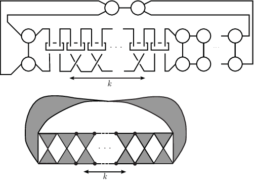
In Figure 14, we depict the shapes of the torus cusps. The left diagram shows the shape of a crossing circle cusp without a half twist below, the middle shows the shape of a crossing circle cusp with a half twist, and the right shows the shape of the cusp which comes from the knot component.

The shape of the torus cusp of the knot component in Figure 13 is obtained by arranging copies of the rectangle in Figure 11 to form a rectangle with opposite edges identified by translations. Therefore, its cusp modulus is . The modulus of each crossing circle cusp depends on the existence of a half twist; if it has a half twist below, the modulus is and if not, it is . (Note that these moduli do not depend on the total number of vertices in the graph .)
8. Construction of different manifolds sharing the same volume
We start with the graph with vertices shown in Figure 15. This graph is obtained by applying the gluing move in Lemma 6.1 times to .

First, we label every remaining pair of thrice punctured spheres by an element of . For each such pair we apply Lemma 6.1 as follows. We glue the pair of thrice punctured spheres labelled by (resp. ) without (resp. with) a half twist, as in Figure 5 (left) (resp.(right)). By this construction, we get a hyperbolic link complement for each cyclic binary word of length and its volume is .
Now we consider the decomposition of into isometric convex hyperbolic polyhedra with shaded faces described in section 6.1. Note that every edge lies in exactly one shaded triangular face, since the faces have a checkerboard colouring.
Definition 8.1 ([20], [39]).
Given an edge in such a polyhedral decomposition, let be the shaded ideal triangle containing . Then the midpoint of is the foot of the perpendicular in from the vertex of opposite to .
Since isometries preserve angles, when we glue two thrice punctured sphere boundaries together by an isometry, it maps midpoints to midpoints. Moreover, for fully augmented links, we may expand horoball neighbourhoods of the cusps to find a horoball packing such that the horoballs bump together precisely at the midpoints of edges. More precisely,
Theorem 8.2 ([20], [39]).
Let be a fully augmented link. Then there exist horoball neighbourhoods of the cusps of such that the midpoint of every edge is a point of tangency of the corresponding horospherical tori.
Remark 8.3.
For each , we fix the horoball packing given by Theorem 8.2. In fact, this horoball packing depends only on the geometry of and not on any choice of polyhedral decomposition for . This follows since the horospherical tori for can be defined as follows: For each cusp with modulus or we choose the horospherical torus of area , and for each cusp with modulus with we choose the horospherical torus of area . These areas are easily calculated from the diagrams in Figures 10–12 and Figure 14, using the fact that each dotted edge in Figures 10-12 has length 1 in the horospherical tori for , (since it is a horocycle joining midpoints of edges in an ideal hyperbolic triangle).
Theorem 8.4.
Let be a binary cyclic word of length and let be the hyperbolic link complement obtained from by the above procedure for . Then is isometric to if and only if and are related by the natural action of , the dihedral group of order .
Proof.
Let be a binary cyclic word of length . If contains zeros, then we can split into subwords of the form with ’s by using each zero in exactly twice.
After the gluing move in Lemma 6.1, each produces a torus cusp with crossings, whose modulus is (see Example 7.1). Let be the decomposition of , and let be the cusp corresponding to the knot component produced by . We get a cyclic sequence of cusp moduli from . Note that the total number of cusps of is ; the crossing circle cusp at the top of Figure 15 has modulus (from the cusp diagram in Figure 12), and the other crossing circle cusps have modulus or by Example 7.1.
We now only consider cusps whose modulus has norm greater than . For , these are the cusps and . From , we will construct a labelled cusp graph with vertices as follows. We label by for and by , the modulus of . Then join and by an edge if in , horoball neighbourhoods of the cusps corresponding to and are tangent to each other. In , the horoball neighbourhood of each cusp bumps only into , (with index modulo ), and . Therefore, the graph consists of a cycle of length whose vertices are labelled cyclically by the ’s and one vertex labelled by joined to every vertex of the cycle.
The special case when and is slightly different. Then has one cusp of modulus as above, two knot components giving cusps of modulus , and cusps of modulus . In this case, the cusp graph is a 3-cycle.
Conversely given such a labelled cusp graph, we can reconstruct a binary cyclic word. Therefore given two binary cyclic words and of length , the graph is isomorphic to as a graph with labelled vertices if and only if is related to by the natural action of . Moreover, by Remark 8.3, any isometry between manifolds and takes the horoball packing to . Hence, the manifold is isometric to if and only if the graph is isomorphic to as a graph with labelled vertices. This completes the proof. ∎
Theorem 8.5.
For each , there are at least different hyperbolic link complements of volume .
Proof.
By theorem 8.4, there are at least as many hyperbolic link complements of volume as cyclic binary words of length , up to the action of . But there are based cyclic binary words of length , and each orbit under the action has at most elements. So the result follows. ∎
Remark 8.6.
For the sequence , this gives a logarithmic growth rate
Chesebro-BeBlois [11] construct examples of hyperbolic link complements of volume , giving a logarithmic growth rate
9. Some Open Questions
- (1)
Find additional exact values of or upper bounds on .
- (2)
(Gromov [24], 1979) Is locally bounded?
This reduces to the question of whether the number of manifolds with a given volume is uniformly bounded amongst all hyperbolic Dehn fillings on any given cusped hyperbolic 3-manifold.
- (3)
What is the largest volume of a closed hyperbolic 3-manifold that does not arise from Dehn filling of or ? (This would allow us to make the result of Theorem 3.1 explicit.)
Experimental evidence suggests that the largest such volume is for the closed manifold . (This is the largest such volume arising in the Hodgson-Weeks census of low volume closed hyperbolic 3-manifolds with shortest closed geodesic of length , and also for Dehn fillings on the “magic manifold” s776.)
- (4)
(i) Are all hyperbolic Dehn fillings on determined by their volumes, amongst Dehn fillings on ?
(ii) Are all hyperbolic Dehn fillings on determined by their volumes, amongst Dehn fillings on ?
(iii) There are some equalities between volumes of Dehn fillings on and , observed in [27], and shown in equation (5.6) above. The Meyerhoff manifold of volume also arises as Dehn filling on both: . Are these the only equalities between volumes of Dehn fillings on and ?(These statements can be checked experimentally using SnapPy and Snap: for instance they are true for all hyperbolic Dehn fillings on and with .)
- (5)
For which cusped hyperbolic 3-manifolds are there infinitely many hyperbolic Dehn fillings on that are uniquely determined by their volumes amongst Dehn fillings on ?
Our methods give some further results on this question when the cusp shape lies in an imaginary quadratic number field. But for algebraic of higher degree, our approach would require new results on the distribution of gaps in the values of the quadratic form for integers . This question also arises in the subject of “Quantum Chaos”, and it is conjectured that the successive gaps should be randomly distributed according to a Poisson distribution (see [42], [41], [16]). This would imply that arbitrarily large 2-sided gaps always exist.
- (6)
Are there sequences with for all ?
- (7)
Are there sequences such that the growth rate of the number of link complements with volume is faster than exponential, i.e with ?
References
- [1] J. W. Aaber and N. M. Dunfield, Closed surface bundles of least volume, Algebr. Geom. Topol. 10 (2010), 2315–2342.
- [2] C. Adams, Thrice-punctured spheres in hyperbolic 3-manifolds, Trans. Amer. Math. Soc. 287 (1985), no. 2, 645-656.
- [3] I. Agol, Bounds on exceptional Dehn filling. Geom. Topol. 4 (2000), 431–449.
- [4] I. Agol, The minimal volume orientable hyperbolic 2-cusped 3-manifolds. Proc. Amer. Math. Soc. 138 (2010), 3723–3732.
- [5] M. Belolipetsky, T. Gelander, A. Lubotzky and A. Shalev, Counting arithmetic lattices and surfaces, Annals of Math. (2) 172 (2010), no. 3, 2197–2221.
- [6] M. Burger, T. Gelander, A. Lubotzky and S. Mozes, Counting hyperbolic manifolds, Geom. Funct. Anal. 12 (2002), 1161–1173.
- [7] D. A. Buell, Binary quadratic forms: Classical theory and modern computations, Springer-Verlag, New York, 1989.
- [8] P. Callahan, M. Hildebrand and J. Weeks, A census of cusped hyperbolic 3-manifolds, Math. Comp. 68 (1999), no. 225, 321–332.
- [9] C. Cao and G. R. Meyerhoff, The orientable cusped hyperbolic 3-manifolds of minimum volume, Invent. Math. 146 (2001), no. 3, 451–478.
- [10] S. Carlip, Dominant topologies in Euclidean quantum gravity, Topology of the Universe Conference (Cleveland, OH, 1997), Classical Quantum Gravity 15 (1998), no. 9, 2629–2638.
- [11] E. Chesebro and J. DeBlois, Algebraic invariants, mutation, and commensurability of link complements, arXiv:1202.0765.
- [12] T. Chinburg, E. Friedman, K. Jones and A. Reid, The arithmetic hyperbolic 3-manifold of smallest volume, Ann. Scuola Norm. Sup. Pisa Cl. Sci. (4) 30 (2001), no. 1, 1–40.
- [13] D. A. Cox, Primes of the form : Fermat, class field theory and complex multiplication, Wiley, New York, 1989.
- [14] M. Culler, N. M. Dunfield, and J. R. Weeks, SnapPy, a computer program for studying the geometry and topology of 3-manifolds. Available at http://snappy.computop.org
- [15] N. M. Dunfield , S. Garoufalidis, A. Shumakovitch and M. Thistlethwaite, Behavior of knot invariants under genus 2 mutation, New York J. Math. 16 (2010), 99-123.
- [16] A. Eskin, G. Margulis and S. Mozes, Quadratic forms of signature (2, 2) and eigenvalue spacings on rectangular 2-tori, Ann. of Math. (2) 161 (2005), no. 2, 679–725.
- [17] R. Frigerio, B. Martelli and C. Petronio, Complexity and Heegaard genus of an infinite class of compact 3-manifolds, Pacific J. Math. 210 (2003), 283–297.
- [18] R. Frigerio, B. Martelli and C. Petronio, Dehn filling of cusped hyperbolic 3-manifolds with geodesic boundary, J. Differ. Geom. 64 (2003), 425-455.
- [19] M. Fujii, Hyperbolic 3-manifolds with totally geodesic boundary which are decomposed into hyperbolic truncated tetrahedra, Tokyo J. Math. 13 (1990), no. 2, 353–373.
- [20] D. Futer and J. S. Purcell, Links with no exceptional surgeries, Comment. Math. Helv. 82 (2007), no. 3, 629-664.
- [21] D. Gabai, G. R.Meyerhoff, P. Milley, Minimum volume cusped hyperbolic three-manifolds, J. Amer. Math. Soc. 22 (2009), 1157–1215.
- [22] D. Gabai, G. R.Meyerhoff, P. Milley, Mom technology and volumes of hyperbolic 3-manifolds, Comment. Math. Helv. 86 (2011), 145–188.
- [23] O. Goodman, Snap, a computer program for studying arithmetic invariants of hyperbolic 3-manifolds. Available from http://www.ms.unimelb.edu.au/snap
- [24] M. Gromov, Hyperbolic manifolds (according to Thurston and Jørgensen), Bourbaki Seminar, Vol. 1979/80, pp. 40–53, Lecture Notes in Math., 842, Springer, Berlin-New York, 1981.
- [25] G. H. Hardy and E. M. Wright, An introduction to the theory of numbers, Oxford University Press, 5th edition, 1979.
- [26] D. Heard, C. Hodgson, B. Martelli, C. Petronio, Hyperbolic graphs of small complexity, Experiment. Math. 19 (2010), 211-236.
- [27] C. Hodgson, R. Meyerhoff and J. Weeks, Surgeries on the Whitehead link yield geometrically similar manifolds, Topology ’90 (Columbus, OH, 1990), 195–206, de Gruyter, Berlin, 1992.
- [28] C. Hodgson and S. Kerckhoff, The shape of hyperbolic Dehn surgery space, Geom. Topol. 12 (2008), no. 2, 1033–1090.
- [29] C. Hodgson and J. Weeks, Symmetries, isometries and length spectra of closed hyperbolic three-manifolds, Experiment. Math. 3 (1994), 261–274.
- [30] S. Kojima and Y. Miyamoto, The smallest hyperbolic 3-manifolds with totally geodesic boundary, J. Differential Geom. 34 (1991), no. 1, 175–192.
- [31] M. Lackenby, Word hyperbolic Dehn surgery, Invent. Math. 140 (2000), no. 2, 243–282.
- [32] M. Lackenby, The volume of hyperbolic alternating link complements, Proc. London Math. Soc. (3) 88 (2004), no. 1, 204-224. With an appendix by I. Agol and D. Thurston.
- [33] E. Landau, Elementary number theory. Chelsea Publishing Co., New York, 1958.
- [34] H. Masai, On volume preserving moves on graphs and their applications, in preparation.
- [35] P. Milley, Minimum volume hyperbolic 3-manifolds, J. Topol. 2 (2009), 181–192.
- [36] Y. Miyamoto, Volumes of hyperbolic manifolds with geodesic boundary, Topology 33 (1994), 613–629.
- [37] W. D. Neumann and A. W. Reid, Arithmetic of Hyperbolic Manifolds, in Topology ’90, Proceedings of the Research Semester in Low Dimensional Topology at Ohio State, de Gruyter, Berlin-New York, 1992, 273–310.
- [38] W. Neumann and D. Zagier, Volumes of hyperbolic three-manifolds, Topology 24 (1985), no. 3, 307–332.
- [39] J. Purcell, An introduction to fully augmented links, Interactions between hyperbolic geometry, quantum topology and number theory, 205–220, Contemp. Math., 541, Amer. Math. Soc., 2011.
- [40] D. Ruberman, Mutation and volumes of knots in , Invent. Math. 90 (1987), no. 1, 189–215.
- [41] Z. Rudnick, What is… quantum chaos?, Notices Amer. Math. Soc. 55 (2008), no. 1, 32–34.
- [42] P. Sarnak, Values at integers of binary quadratic forms, in Harmonic analysis and number theory (Montreal, PQ, 1996), 181–203, CMS Conf. Proc., 21, Amer. Math. Soc., 1997.
- [43] W. Thurston, Geometry and topology of 3-manifolds, Lecture notes, Princeton University, 1978.
- [44] J. R. Weeks, Hyperbolic structures on 3-manifolds, Ph.D. thesis, Princeton University, 1985.
- [45] J. R. Weeks, SnapPea: A computer program for creating and studying hyperbolic 3- manifolds. Available at http://www.geometrygames.org/SnapPea/
- [46] N. Wielenberg, Hyperbolic 3-manifolds which share a fundamental polyhedron, Riemann Surfaces and Related Topics: Proceedings of the 1978 Stony Brook Conference, Princeton Univ. Press, Princeton, N. J., 1981, pp. 505-513.
- [47] B. Zimmermann, A note on hyperbolic 3-manifolds of the same volume, Monaths. Math., 110 (1990), pp. 321-327.