Joint Base Station Clustering and Beamformer Design for Partial Coordinated Transmission in Heterogeneous Networks
Abstract
We consider the interference management problem in a multicell MIMO heterogeneous network. Within each cell there is a large number of distributed micro/pico base stations (BSs) that can be potentially coordinated for joint transmission. To reduce coordination overhead, we consider user-centric BS clustering so that each user is served by only a small number of (potentially overlapping) BSs. Thus, given the channel state information, our objective is to jointly design the BS clustering and the linear beamformers for all BSs in the network. In this paper, we formulate this problem from a sparse optimization perspective, and propose an efficient algorithm that is based on iteratively solving a sequence of group LASSO problems. A novel feature of the proposed algorithm is that it performs BS clustering and beamformer design jointly rather than separately as is done in the existing approaches for partial coordinated transmission. Moreover, the cluster size can be controlled by adjusting a single penalty parameter in the nonsmooth regularized utility function. The convergence of the proposed algorithm (to a stationary solution) is guaranteed, and its effectiveness is demonstrated via extensive simulation.
I Introduction
The design of future wireless cellular networks is on the verge of a major paradigm change. In order to accommodate the explosive demand for wireless data, the traditional wireless network architecture comprised of a small number of high power base stations (BSs) has started to migrate to the so-called heterogeneous network (HetNet) [1, 2]. In HetNet, each cell is composed of potentially a large number of densely deployed access nodes such as macro/micro/pico BSs to provide coverage extension for cell edge and hotspot users [2]. Unfortunately, close proximity of many transmitters and receivers introduces substantial interference, which, if not properly managed, can significantly affect the system performance.
The interference management problem in multicell downlink networks has been a topic of intensive research recently. It has been widely accepted that combining physical layer techniques such as multiple input multiple output (MIMO) antenna arrays with multi-cell coordination can effectively mitigate inter-cell and intra-cell interference [3, 4, 5]. There are two main approaches for the coordinated transmission and reception in a multi-cell MIMO network: joint processing (JP) and coordinated beamforming (CB) [3]. In the first approach, the user data signals are shared among the cooperating BSs. A single virtual BS can then be formed that transmits to all the users in the system. Inter-BS interference is canceled by joint precoding and transmission among all the coordinated BSs. In this case, either the capacity achieving non-linear dirty-paper coding (DPC) (see, e.g., [6, 7]), or simpler linear precoding schemes such as zero-forcing (ZF) (see, e.g., [8, 9, 10]) can be used for joint transmission. However, centralized processing is needed for the computation of the beamformers. Furthermore, this approach can require heavy signaling overhead on the backhaul network ([11, 5, 12]) especially when the number of cooperating BSs in the network becomes large.
When the benefit of full JP among the BSs is outweighed by the overhead, the BSs can choose CB as an alternative reduced coordination scheme. In particular, the beamformers are jointly optimized among the coordinated BSs to suppress excessive inter-BS interference. In this case, only local channel state information (CSI) and control information are exchanged among the coordinated BSs. One popular formulation for CB is to optimize the system performance measured by a certain system utility function. Unfortunately, optimally solving the utility maximization problem in MIMO interfering network is computationally intractable in general (except for a few exceptions, see [13, 14, 15, 16]). As a result, many works are devoted to finding high quality locally optimal solutions for different network configurations, e.g., in MIMO/MISO interference channels (IC), [17, 18, 19, 20, 21] and MIMO/MISO interfering broadcast channels (IBC) [22, 23, 24]. In particular, reference [24] proposed a weighted Minimum Mean Square Error (WMMSE) algorithm that is able to compute locally optimal solutions for a broad class of system utility functions and for general network configurations.
A different approach for limited coordination is to group the BSs into coordination clusters of small sizes, within which they perform JP. In this case, each user’s data signals are only shared among a small number of its serving BSs, thus greatly reducing the overall backhaul signaling cost. Many recent works have developed various BS clustering strategies for such purpose, e.g., [9, 25, 26, 27, 28, 29, 30, 31], where clusters are formed either greedily or by an exhaustive search procedure. Once the clusters are formed, various approaches can be used to design beamforming strategies for each BS. For example, the authors of [28, 29, 30] utilized the ZF strategy for intra-cluster transmission without assuming any inter-cluster cooperation. References [9, 25] considered a hybrid cooperation strategy in which CB is used for inter-cluster coordination. In this way, inter-cluster interference for cluster edge users is also mitigated. In principle, clustering strategies should be designed in conjunction with the beamforming and BS coordination strategies to strike the best tradeoff among system throughput performance and signalling overhead.
In this work, we consider the joint BS clustering and beamformer design problem in a downlink multicell HetNet for general partial coordinated transmission. In our formulation, the BSs that belong to the same cell can dynamically form (possibly overlapping) coordination clusters of small sizes for JP while the BSs in different cells perform CB. We formulate this problem from the perspective of sparse optimization. Specifically, if all the BSs that belong to the same cell are viewed as a single virtual BS, then its antennas can be partitioned into multiple groups (each corresponding to an individual BS). Moreover, the requirement that each user is served by a small number of BSs translates directly to the restriction that its virtual beamformer should have a group sparse structure, that is, the nonzero components of the virtual beamformer should correspond to only a small number of antenna groups. This interpretation inspires us to formulate a system utility maximization problem with a mixed regularization, as it is well known that such regularization induces the group sparse structure [32]. Incorporating such nonsmooth regularization term into our objective ensures that the optimal beamformers possess the desired group-sparse structure. In this way, our proposed approach can be viewed as a single-stage formulation of the joint BS grouping and beamforming problem. The main contributions of this work are listed as follows.
- •
We propose to jointly optimize the coordination clusters and linear beamformers in a large scale HetNet by solving a single-stage nonsmooth utility optimization problem. The system utility function (without nonsmooth penalization) can have a very general form that includes the popular weighted sum rate and proportional fair utility functions. This approach is different from the existing algorithms, which either require a predefined BS clustering and a fixed system utility function, or some multi-stage heuristic optimization.
- •
Since the resulting nonsmooth utility maximization problem is difficult to solve due to its nonconvexity as well as its nonsmoothness, we transform this problem to an equivalent regularized weighted MSE minimization problem. The latter has several desirable features such as separability across the cells and convexity among different blocks of variables. This equivalence transformation substantially generalizes our previous result in [24], which only deals with smooth utility functions.
- •
We propose an efficient iterative algorithm that computes a stationary solution to the transformed problem. In each step of the algorithm the computation is closed-form and can be distributed to individual cells. The algorithm is shown to converge to a stationary solution to the original nonsmooth utility maximization problem, and its effectiveness is demonstrated via extensive simulation experiments.
The rest of the paper is organized as follows. In Section II, we present the system model and formulate the problem into a nonsmooth utility maximization problem. We then transform this problem into an equivalent regularized weighted MSE minimization problem in Section III. In Section IV, an efficient algorithm is proposed to solve the transformed problem. In Section V, numerical examples are provided to validate the proposed algorithm.
Notations: For a symmetric matrix , signifies that is positive semi-definite. We use , , and to denote the trace, determinant, hermitian and spectral radius of a matrix, respectively. For a complex scalar , its complex conjugate is denoted by . For a vector , we use to denote its norm. is used to denote a identity matrix. We use to denote a vector with its th element replaced by . We use and to denote the set of real and complex matrices; We use and to denote the set of hermitian and hermitian positive semi-definite matrices, respectively. We use the expression: to indicate .
II System Model and Problem Formulation
Consider a downlink multi-cell HetNet consisting of a set of cells. Within each cell there is a set of distributed base stations (BS) (for instance, macro/micro/pico BSs) which provide service to users located in different areas of the cell. Assume that in each cell , there is low-latency backhaul network connecting the set of BSs to a central controller (usually the macro BS), and that the central controller makes the resource allocation decisions for all BSs within the cell. Furthermore, this central entity has access to the data signals of all the users in its cell. Let denote the users located in cell . Each of the users is served jointly by a subset of BSs in . Let denote the set of all the users. For simplicity of notations, let us assume that each BS has transmit antennas, and each user has receive antennas. Throughout the paper, we use to indicate the user index, use for the cell index, and use for the BS index. Let denote the channel matrix between the th BS in the th cell and the th user in the th cell. Let denote the channel matrix between all the BSs in the th cell to the user .
Let denote the transmit beamformer that BS uses to transmit a single stream of data signal to user . Define as the collection of all beamformers intended for user . Let . Assume that there is a power budget constraint for each BS , i.e.,
| (1) |
Let denote the transmitted signal of BS , and let denote the collection of transmitted signals of all the BSs in cell , i.e.
The received signal of user is
| (2) |
where is the additive white Gaussian noise with distribution .
Let denote the receive beamformer used by user to decode the intended signal. Then the estimated signal for user is: . The mean square error (MSE) for user can be written as
| (3) |
The MMSE receiver minimizes user ’s MSE, and can be expressed as
| (4) |
where denotes user ’s received signal covariance matrix. The minimum MSE for user when the MSE receiver is used can be expressed as
| (5) |
Clearly, we have . Let us assume that Gaussian signaling is used and the interference is treated as noise. If we assume that all the BSs in cell form a single virtual BS, then can be viewed as the virtual beamformer for user . The achievable rate for user is given by [33]
| (6) |
The above expression suggests that each user can always use a MMSE receiver (4) since it preserves achievable data rate when the interference is treated simply as noise. We will occasionally use the notations , to make their dependencies on explicit.
Notice that the rate (6) can only be achieved when all the BSs in cell perform a full JP. Unfortunately, this requires the data signal for user to be known at all BSs in , causing significant signaling overhead, especially when the number of users and BSs becomes large. To reduce overhead, partial cooperative transmission is preferred whereby each user is served by not all, but a subset, of BSs in the cell. Mathematically, we are interested in jointly performing the following two tasks: i) for each user , identify a small subset of serving BSs such that for each , ; ii) optimize the transmit beamformers to achieve high system throughput and/or fairness level. With the partial JP, user ’s data signal needs to be shared only among BSs in , rather than among all BSs in .
The requirement that is small translates to the restriction that should contain only a few nonzero block components (i.e., most of the beamformers should be set to zero). This structure of the beamformer is referred to as the group sparse structure [32]. Recovering group sparse solutions for optimization problem has recently found its application in many fields such as machine learning [34], microarray data analysis [35], signal processing [36, 37] and communications [38]. One popular approach to enforce the sparsity of the solution to an optimization problem is to penalize the objective function with a group-sparse encouraging penalty such as the mixed norm [32]. In our case, such norm can be expressed as: , which is the norm of the vector consists of norms . The resulting penalized problem is usually referred to as the group least-absolute shrinkage and selection operator (LASSO) problem.
With the goal of inducing group-sparse structure of the beamformers as well as optimizing system-level performance, we propose to design the linear transmit beamformers by solving the following problem
| (7) | ||||
where denotes user ’s utility function, and is the set of parameters that control the level of sparsity within each cell. Penalizing the objective with the nonsmooth mixed norm induces the group sparsity of . To see this, note that the group sparsity of can be characterized by the sparsity of the vector , and the norm of this vector, which is what we use in (7), is a good approximation of the norm of it (defined as the number of nonzero entries of the vector); see the literature on compressive sensing [39]. The reference [32] contains more discussion on using the mixed norm to recover the group sparsity.
Unfortunately, solving directly is challenging. One reason is that when , (P1) becomes a sum utility maximization problem for an interfering broadcast channel, which is proven to be NP-hard for many common utility functions (see [13, 14, 15, 16]). Another reason is that most existing algorithms for solving the nonsmooth group LASSO problem such as [32, 40, 41, 36] only work for the case that the smooth part of the objective is convex and quadratic. We will provide in the next section an equivalent reformulation of this problem in which these difficulties are circumvented. The reformulated problem can be solved (to a stationary solution) via solving a series of convex problems.
III Equivalent Formulation
In this section, we develop a general equivalence relationship between the utility maximization problem and a regularized weighted MSE minimization problem. This result is a generalization of a recent equivalence relationship developed in [24] to the nonsmooth setting. The proofs of the results in this section can be found in Appendix A.
III-A Single User Per Cell with Sum Rate Utility
For ease of presentation, we first consider a simpler case in which there is a single user in each cell. This scenario is of interest when different mobiles in each cell are scheduled to orthogonal time/frequency resources, and we consider one of such resources. We also focus on using the sum rate utility function. Generalizations to multiple users per-cell case with more general utility functions will be given in the next subsection.
Now that there is a single user in each cell, we denote the user in th cell as user . We use and to denote the BS ’s beamformer for user , and the channel from BS to user , respectively. Define , , , and similarly. Using the sum rate as the system utility function, the sparse beamforming problem for this network configuration is given as
| (8) | ||||
Let us introduce a set of new weight variables . Consider the following regularized weighted MSE minimization problem
| (9) | ||||
One immediate observation is that fixing and solving for admits a closed form solution: . Such property will be used in the following to derive the equivalence relationship between problems (8) and (9). We refer the readers to [24, Section II.A] for a simple example that motivates this equivalence in the case .
To formally derive the equivalence relationship, the following definitions (see [42]) of stationary points of a nonsmooth function are needed. Note that stationarity is a necessary condition for both global and local optimality. Let be a vector of variables, in which . Let be a real valued (possibly nonsmooth) continuous function.
Definition 1
is a stationary point of the problem if and , where is the directional derivative of at in the direction
Definition 2
is a coordinatewise stationary point of if and
where denotes a vector with all zero components except for its th block.
Definition 3
The function is regular at if implies .
Proposition 1
III-B Multiple Users Per Cell with More General Utility
In this section, we generalize the equivalence relationship presented in the previous section to the case with more general utility function and multiple users per cell.
Consider the utility function that satisfies the following two conditions:
- C1)
-
is concave and strictly increasing in ;
- C2)
-
is strictly convex in for all satisfying .
Note that this family of utility functions includes several well known utilities such as weighted sum rate and geometric mean of one plus rates [24]. Let be a set of real-valued weights. Let denote the inverse function of the derivative . Consider the following regularized weighted MSE minimization problem
Similar to Proposition 1, we can establish the following equivalence relationship.
Proposition 2
Suppose for each , the utility function satisfies the conditions C1)–C2). If is a stationary solution to problem , then must be a stationary solution to problem . Conversely, if is a stationary solution to problem , then the tuple must be a stationary solution to problem , where
Moreover, the global optimal solutions for these two problems are identical.
We remark that is again the MSE receiver corresponding to ; takes a similar form to that in the statement of Proposition 1, except for the inclusion of a positive weight . The positivity of comes form the assumption C1).
IV Joint Clustering and Beamformer Design
In this section, we will develop an efficient iterative algorithm for the general nonsmooth utility maximization problem . Due to the equivalence of this problem and the regularized weighted sum-MSE minimization problem , we can focus on solving the latter. We will employ the block coordinate descent (BCD) method [42] for such purpose.
IV-A The Algorithm
It is straightforward to verify that the objective of problem is convex w.r.t. each variable . When are fixed, the optimal is the MMSE receiver . When are fixed, the optimal takes the following form
The positivity of comes from the fact that and the utility function is strictly increasing w.r.t. user ’s rate.
The main part of the algorithm is to find the optimal transmit beamformers when are fixed. Observe that when fixing , problem can be decomposed into independent convex problems (one for each cell)
Let us focus on solving one of such problems. Note that the constraint set of this problem is separable among the beamformers of different BSs. This suggests that we can obtain its optimal solution again by a BCD method, with as one block of variables. In particular, we will solve (P3) by sequentially solving the following problem for each block
This problem is a quadratically constrained group-LASSO problem. The presence of the additional sum power constraint prevents the direct application of the algorithms (e.g., [32, 40, 41, 36]) for conventional unconstrained group-LASSO problem. In the following we will derive a customized algorithm for solving this problem.
Define the following two sets of variables
| (10) | ||||
| (11) |
Partition and into the following form
| (15) |
where , and . Utilizing these definitions, the objective of problem (P4) reduces to
The gradient of the smooth function w.r.t. can be expressed as
| (16) | ||||
| (17) |
where we have defined
| (18) |
Note that the gradient (16) given above is coupled with other block variables , through the term .
The first order optimality condition for the convex problem (P4) is
| (19) | ||||
| (20) |
where is the Lagrangian multiplier for BS ’s power budget constraint; represents the subdifferential of the nonsmooth function at the point . The latter can be expressed as follows (see [32, 43])
Finding the global optimal solution of problem (P4) amounts to finding the optimal primal dual pair that satisfy the conditions (19)–(20). In the following, we will first develop a procedure to find that satisfy the conditions (19) for a given . Then we will use a bisection method to search for the optimal multiplier.
Step 1) Utilizing the expression for the subdifferential in (IV-A), the optimality condition (19) can be rewritten as [32, 43]
| (23) | ||||
| (24) |
with defined as . Note that (23) is the key to achieve sparsity, as whenever is less than the threshold , will be forced to . The correctness of (24) can be checked by plugging the second part of (IV-A) into (19).
By definition, the optimal must satisfy
| (25) |
Define the set of active users for BS as , and define its cardinality as . For any given , let us denote a beamformer that satisfies (23)-(24) as , and the corresponding that satisfies (25) as . Clearly for a user that satisfies the condition (23) (i.e., ), does not depend on and can be directly computed. Let us then focus on the active user . For any , finding a amounts to obtaining the corresponding that satisfies (25). Due to a certain monotonicity property of the function w.r.t. , a bisection search on can be used to find . This claim is established in Appendix B. Once is found for all , we can use (24) to find .
Step 2) Once is obtained, we need to search for the optimal that satisfies the feasibility and the complementarity condition (20). The following result (the proof of which can be found in Appendix C) suggests that there must exist a such that the optimal multiplier must lie in . Moreover, we can perform a bisection search to find the optimal multiplier.
Lemma 1
Performing Step 1) and Step 2) iteratively, we can find the desired optimal primal-dual pair for problem (P4). Table I summarizes the above BCD procedure.
| S1) Initialization Generate a feasible set of beamformers |
| S2) Compute and using (10) and (11) |
| S3) Repeat Cyclically pick a BS |
| S4) Compute using (18) for each |
| If set |
| Else, choose and such that |
| S5) Repeat |
| S6) For each , choose and such that |
| S7) Repeat (for each ) , |
| S8) |
| S9) If , ; Otherwise, |
| S10) Until |
| S11) If , ; Otherwise, |
| S12) Until |
| S13) |
| End If |
| S14) Until Desired stopping criteria is met |
It is worth noting that the algorithm in Table I admits a particular simple form (without performing the bisection steps) when there is a single user in each cell, and each BS has a single antenna. Let us again denote the only user in the th cell as user . The procedure to find BS ’s scalar beamformer for user (i.e., Step S4–S13 in Table I) can be simplified as follows. Utilizing (23)–(24), if , . Otherwise, note that in this case, we have
| (26) |
Consequently, we obtain a closed-form expression for : . Substituting this into (24), we obtain
where the multiplier should be chosen such that the condition (20) is satisfied. In summary, we have the following closed-form solution for updating
The complete algorithm for solving the regularized weighted MSE minimization problem is given in Table II. We name this algorithm sparse weighted MMSE algorithm (S-WMMSE). The following theorem states its convergence property. The proof can be found in Appendix D.
Theorem 1
The S-WMMSE algorithm converges to a stationary solution of problem .
| S1) Initialization Generate a feasible set of variables |
| S2) Repeat |
| S3) |
| S4) , |
| S5) For each , update using Table I. |
| S6) Until Desired stopping criteria is met |
IV-B Parameter Selection
In this subsection, we provide guidelines for choosing some key parameters for practical implementation of the proposed algorithm.
When are fixed, the procedure in Table I contains two bisection loops for solving for each . The outer loop searches the optimal that ensures satisfy the complementarity and feasibility conditions (20). The inner loop searches for the optimal to ensure (25). In implementation, it will be useful to have explicit expressions for initial bounds of these variables.
IV-B1 The Choice of Initial
From the fact that , we can simply set the lower bound as . For the initial upper bound , it is sufficient to guarantee that
| (30) |
To see this, recall that is monotonically decreasing w.r.t. . Consequently when (30) is satisfied, there must exist a such that both the feasibility and complementarity condition (20) is satisfied.
To ensure (30), it is sufficient that such satisfies the following condition for each active user (notice that the active set is decided before bisection starts)
For a specific , we have the following inequalities
| (31) | ||||
where in we have used the fact that (31) is decreasing w.r.t. ; in we have used the fact that . As a result, it is sufficient to find a such that for all . This implies that the following choice ensures (30)
| (32) |
IV-B2 The Choice of Initial ,
Once the initial bounds on are chosen, we can determine the initial bounds for each , . Because , the lower bound can be simply set as . Next, we will find the that is suitable for all . From the proof of Lemma 3, we see that it is sufficient to choose the initial bound such that
| (33) |
In this way for each there is a that ensures .
IV-C Distributed Implementation
Suppose that there is some central entity, say a macro BS, managing the downlink resource allocation for each cell. Then under the following assumptions, the proposed algorithm can be implemented distributedly by each macro BS.
- A-1)
-
each macro BS knows the channels from the BSs in its cell to all the users ;
- A-2)
-
each user has an additional channel to feedback information to its current serving BS;
- A-3)
-
different macro BSs can exchange control information.
Under these assumptions, in each iteration of the algorithm, a user can measure the covariance of the received signal and update its weight and receive beamformer , respectively. It then feeds these variables to one of its serving BS, who in turn forwards it to the macro BS. Each pair of macro BSs then exchange their respective users’ current beamformers. With these pieces of information, all macro BSs can carry out the procedure in Table I independently. The newly computed beamforming and clustering decisions are subsequently distributed to the BSs in their respective cells via low-latency backhaul links.
In practice, considering the costs of obtaining and sharing of the channel state information, the sparse clustering algorithm may only need to be executed in its full generality in every several transmission time intervals (TTIs). During the TTIs in which the clustering is kept fixed, one can either keep updating the beamformers (by solving problem (P1) without the regularization term), or even fix the beamformers.
V Numerical Results
In this section, we perform numerical evaluation of our proposed algorithm. We consider a multicell network of up to cells. The distance of the centers of two adjacent cells is set to be meters (see Fig. 1 for an illustration). We place the BSs and users randomly in each cell. Let denote the distance between BS and user . The channel coefficients between user and BS are modeled as zero mean circularly symmetric complex Gaussian vector with as variance for both real and imaginary dimensions, where is a real Gaussian random variable modeling the shadowing effect. We fix the environment noise power for all the users as , fix the power budget of each BSs as , and fix the number of BSs and the number of users in each cell as , . We define .

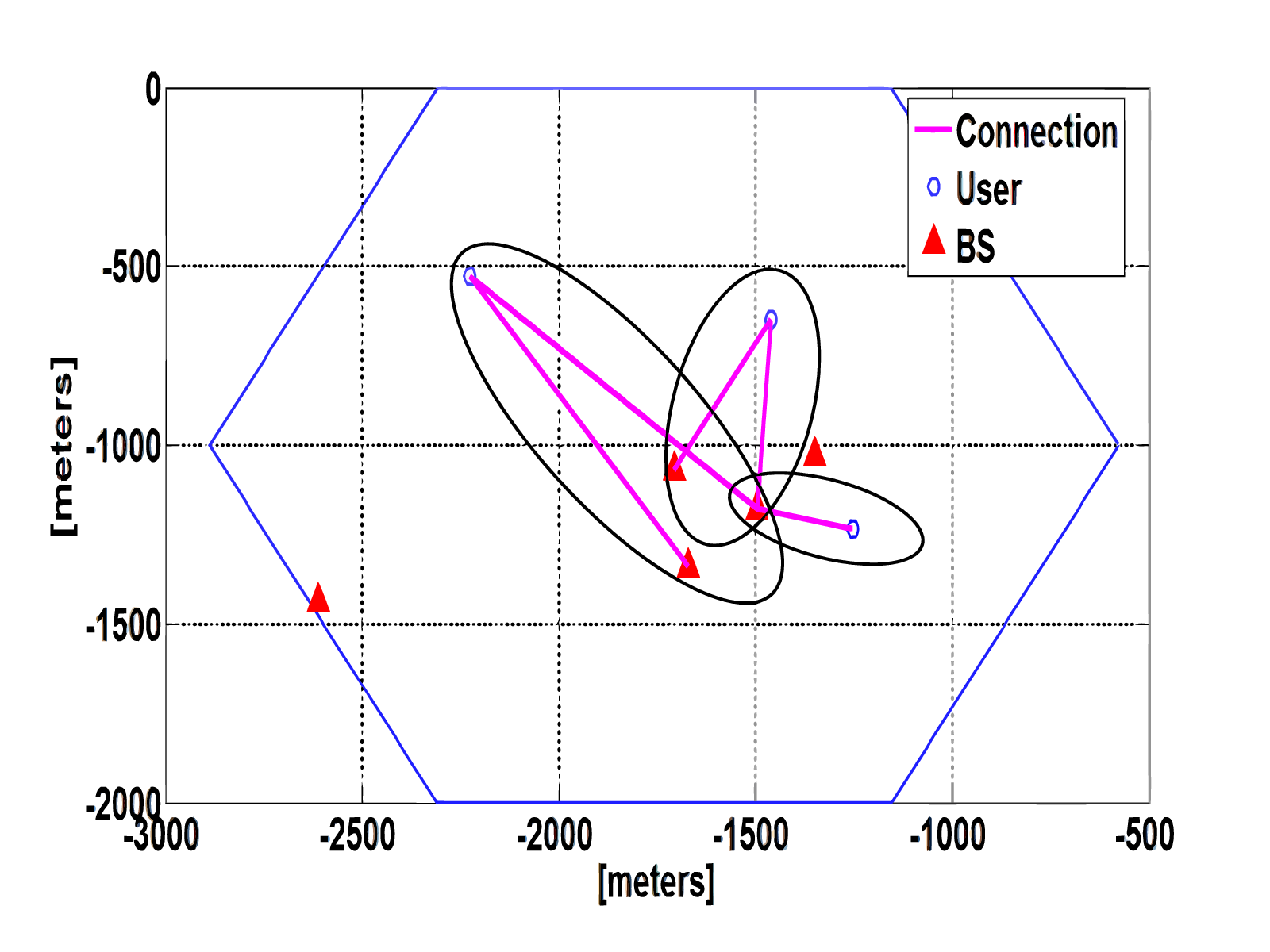
In Fig. 3, we illustrate the structure of the overlapping clusters generated by the S-WMMSE algorithm in a simple single cell network. In this example, when no group-sparsity is considered, each user is served by all the BSs in the set . In contrast, when the clusters are formed by performing the proposed algorithm, the cluster sizes are significantly reduced. In Fig. 3, we show the averaged number of iterations11 1 Note that the number of iterations refer to the outer iterations specified by the update in Table II. needed for the proposed algorithm to reach convergence in different network scenarios. The stopping criteria is set as , where represents the objective value of problem (P1). For both of these results, the sum rate utility is used.
Our experiments mainly compare the proposed algorithm with the following three algorithms:
- •
WMMSE with full intra-cell and limited inter-cell coordination [24]: In this algorithm, the network is modeled as a MIMO-IBC where all the BSs in cell collectively form a giant virtual BS with the transmit power pooled together. It is shown in [24] that this algorithm compares favorably to other popular beamformer design algorithms such as the iterative pricing algorithm [17]. In the present paper, it corresponds to the case where a single cluster is formed in each cell. This algorithm serves as a performance upperbound (in terms of throughput) of the proposed algorithm.
- •
ZF beamforming with heuristic BS clustering: In this algorithm, cooperation clusters with fixed sizes are formed within each BS, and each cluster performs ZF beamforming. The clusters are formed greedily by choosing an initial BS among the unclustered BSs and adding its nearest BSs until reaching the prescribed cluster size. The users are assigned to the cluster with the strongest direct channel (in terms of 2-norm). Each cluster serves its associated users by a single cell ZF linear beamforming [8] 22 2 Note that in [8], after the beams are calculated and fixed, the power allocation for different beams/streams are determined by solving a convex vector optimization with sum-power constraint. In our simulation, we replace the sum-power constraint with a set of per-group of antenna power constraint to better fit the multi-BS setting. . To ensure feasibility of the per-cluster ZF scheme, the weakest users in terms of direct channel are dropped when infeasibility arises.
- •
WMMSE with each user served by its nearest BS: In this algorithm, each user is assigned to the nearest BS, that is, the size of the coordination cluster is at most . We denote this algorithm as WMMSE-nearest neighbor (NN).


We first consider a network with , , , , . We use system sum rate as the utility function. The achieved system sum rate and the averaged number of serving BSs are shown in Fig. 5– Fig. 5 for different algorithms. Each point in the figures is an average of runs of the algorithms over randomly generated networks. Notice that for the ZF based scheme, although the cluster size is given and fixed, the actual number of serving BSs per user can be smaller than the cluster size, as some users may not be served by all the BSs in its serving cluster. It can be seen from Fig. 5– Fig. 5 that the system throughput obtained by the proposed S-WMMSE algorithm is close to what is achievable by the full cooperation. Moreover, the high throughput is achieved using moderate cluster sizes. Notice that the proposed algorithm compares favorably even with the full per-cell ZF scheme (with cluster size ). This suggests that the inter-cluster interference should be carefully taken into consideration when jointly optimizing the BS clusters and beamformers.
It is important to emphasize that the parameters in the proposed algorithm balance the sizes of the clusters and the system throughput. For different network configurations they need to be properly chosen to yield the best tradeoff. Empirically, we found that setting gives a satisfactory tradeoff (as illustrated in Fig. 5– Fig. 5). This is partly because choosing inversely proportional to can better balance the relative importance of the penalization term and the sum rate term when SNR becomes large. To better select this parameter for different system settings, we provide an alternative scheme that adaptively computes in each iteration of the algorithm. Note that for the quadratic problem (P4), if is chosen large enough such that , then . This result can be straightforwardly derived from the optimality condition (23). For conventional quadratic LASSO problem, the fixed sparsity parameter can be chosen as , where is a small number, see, e.g., [36]. In our experiments, we found that choosing as works well for all network configurations. The performance of the S-WMMSE algorithm with this adaptive choices of is also demonstrated in Fig. 5–Fig. 5. Clearly such adaptive choice of can generate smaller sizes of the clusters while achieving similar performance as its fixed parameter counterparts. Note that the convergence proof for the proposed algorithm does not apply anymore, as it requires that parameters must be fixed during the iterations (although in simulation experiments we observe that this adaptive algorithm usually converges).


We also consider a larger network with , , and , and choose to optimize the proportional fairness utility defined as . In Fig. 7–Fig. 9, we compare the performance of the WMMSE algorithm and the WMMSE-NN algorithm33 3 We do not consider the ZF scheme in this experiment for the reason that it cannot guarantee that all the users in the system are served simultaneously, as required by the solution of the proportional fair utility maximization problem. with the proposed algorithm for different choices of . In order to highlight the role of in balancing the system throughput and the cluster sizes, we show in these figures the performance of the proposed algorithm with fixed sparsity parameter for all SNR values. In Fig. 7, we plot the averaged per-BS power consumption relative to that of the WMMSE algorithm. In Fig. 9 we plot the distribution of the individual users’ rates generated by these algorithms. Clearly the proposed algorithm is able to achieve high levels of system throughput and fairness by only using small cluster sizes and significantly lower transmission power (the reduction of transmission power can also be attributed to the use of penalization, see Fig. 7). Additionally, in Fig. 7 and Fig. 9, we include the performance of a limited cooperation scheme in which each cell only coordinates with its nearest neighbor, while treating the signals of the remaining cells as thermal noise (this scheme is labeled as “Sparse-Neighbor”). We observed that this scheme has similar system throughput as the original one, but results in larger cluster size. Such increase in cluster size can be seen as a compensation adopted by the “Sparse-Neighbor” algorithm for ignoring certain inter-cell interference. Due to the limited coordination among the cells, the convergence of this scheme is not theoretically guaranteed. However in simulation we found that the algorithm usually converges.
VI Concluding Remarks
In this work, we propose to jointly optimize the BS clustering and downlink linear beamformer in a large scale HetNet by solving a nonsmooth utility maximization problem. A key observation that motivates this work is that when all the BSs in each cell is viewed as a single virtual BS, the limited coordination strategy that requires a few BSs jointly transmit to a user is equivalent to a group-sparsity structure of the virtual BSs’ beamformers. We effectively incorporate such group-sparsity into our beamformer design by penalizing the system utility function using a mixed norm. We derive a useful equivalent reformulation of this nonsmooth utility maximization problem, which facilitates the design of an efficient iterative group-LASSO based algorithm. Simulation results show that the proposed algorithm is able to select a few serving BSs for each user, while incurring minor loss in terms of system throughput and/or user fairness.
Our framework can be extended for the scenario that multiple streams are transmitted to each user as well. In this more general case, a precoding matrix is used by each BS for each user. To induce sparsity, the utility function should be penalized by the Frobenius norms of the precoding matrices. All the equivalence results derived in Section III hold true for this general case, while the algorithm needs to be properly tailored. We also expect that the proposed approach can be extended for other related problems such as the design of coordinated transceiver in an uplink HetNet, or the design of antenna selection algorithms for large scale distributed antenna systems.
VII Acknowledgement
We wish to thank the anonymous reviewers for their comments that improve the presentation of the paper. The first author also wishes to thank Dr. Qiang Li from Chinese University of Hong Kong and Dr. Ya-feng Liu from Chinese Academy of Sciences for many helpful discussions.
Appendix A Proof of Proposition 1 and Proposition 2
Proof of Proposition 1: Let denote the (nonsmooth) indicator function for the feasible space of vector , i.e.,
We can then rewrite problem (8) compactly as an unconstrained nonsmooth optimization problem
| (36) |
and rewrite (9) equivalently as
| (37) |
We first claim that the function is regular in the sense of Definition 3, under the block structure . This claim can be verified by observing that under such block structure, the nonsmooth parts of the function are separable across blocks, and the smooth part of is differentiable. This property ensures that a coordinatewise stationary point of is also a stationary point. See [42, Lemma 3.1] for a derivation. Similarly, the function is regular under the following block structure
Now assume that is a stationary solution of problem (37), then we must have
| (38) | ||||
| (39) |
where is a vector of zero entries except for the block corresponding to the variable , which takes the value . Condition (38) implies that is the unconstrained local minimum of the function . The same is true for . Notice that is smooth w.r.t. and , consequently, we must have
The above two sets of conditions imply that
In the sequel we will occasionally use and to emphasize their dependencies on . Using these two expressions, we have
| (40) |
where in we have used the matrix inversion lemma [44] to obtain
Using Definition 1, we write the stationarity condition of problem (37) w.r.t. each component as
| (41) |
Using Danskin’s Theorem [45] and the fact that , we have
Combining (41) and the regularity of given in Definition 3, we conclude that
| (42) |
According to Definition 1, satisfies the stationarity condition for problem (36). The reverse direction can be obtained using the same argument.
The equivalence of the global optimal solutions of the two problems can be argued as follows. Suppose is a global optimal solution of but is not a global optimal solution of . Then there must exist a such that . Using (40), we must have . Notice that when plugging , , into , we again have
| (43) |
Therefore, we have
| (44) |
a contradiction to the global optimality of . This completes the second part of the claim.
Proof of Proposition 2 (sketch) We first show that the function is well defined. From our assumption on the utility function , we see that is a strictly convex function in for all . This ensures is a strictly decreasing function. Consequently, its inverse function is well defined. Assume that is a stationary solution to problem . Following the steps of the proof in Proposition 1, we can show that is of the following form
The rest of the proof is the same as that of Proposition 1. We omit it due to space limit.
Appendix B
We first show a monotonicity property of .
Lemma 2
Suppose . Then for fixed , is a strictly decreasing function of . For fixed , is a strictly increasing function of .
Proof:
Define . Then we have
Notice that because it is a principal submatrix of a positive semidefinite matrix . This fact combined with ensures and . Using the fact that and , we have
This condition ensures , , which in turn implies the desired monotonicity.
The second part of the lemma can be shown similarly. ∎
Utilizing Lemma 2, we can show that always exists.
Lemma 3
Suppose the condition is satisfied. Then for any fixed that satisfies , there always exists a that satisfies (25) for all .
Proof:
Pick an . First notice that . We then show that . To this end, we can write
where the last inequality is from the assumption.
Appendix C Proof of Lemma 1
Fix a given , pick . Suppose satisfies . Fix . From Lemma 2 we have . To ensure , we must have , which gives the first part of the claim.
We prove the second part of the claim by contradiction. First consider the trivial case where no user is active, i.e., . Clearly and the claim is proven.
Now suppose is nonempty, that is, . Suppose that there exists an such that for all , . This assumption combined with Lemma 2 implies
| (45) |
However, we have that
which contradicts (45). This suggests that for each , there exists a such that for all , (i.e., ). Taking , we have that for all , . This condition implies that As a result, the second part of the claim is proved.
Appendix D Proof of Theorem 1
Proof:
Due to the equivalence relationship, it is sufficient to show that the S-WMMSE algorithm converges to a stationary solution of the problem .
We first show that the BCD procedure in Table I for updating converges to the global optimal solution of problem (P3). Recall that this problem can be decomposed into independent convex subproblems of the form (P4), then it is sufficient to show that each of these problems are solved globally. Similarly as (36)-(37), problem (P4) can be expressed in its unconstrained form
The procedure in Table I is a BCD method for solving the above unconstrained problem, where each block is defined as . Observe that i) the nonsmooth part of the objective is separable across the blocks; ii) the smooth part of the objective is differentiable; iii) each block variable can be solve uniquely when fixing other variables . According to [42, Theorem 4.1-(c)], these facts are sufficient to guarantee the convergence of this BCD procedure to a global optimal solution of the convex nonsmooth problem (P4).
To prove the convergence of the S-WMMSE algorithm to a stationary solution of problem , we can again write problem into its unconstrained form, and see that the nonsmooth part of the objective is separable across the blocks of variables . Furthermore, when we fix any two block variables and solve for the third, a unique optimal solution can be obtained. Applying [42, Theorem 4.1], we conclude that the S-WMMSE algorithm converges to a stationary solution of the problem (P2). ∎
References
- [1] 3GPP, “Evolved Universal Terrestrial Radio Access (EUTRA) and Evolved Universal Terrestrial Radio Access Network (EUTRAN); overall description,” 2011, 3GPP TS 36.300, V8.9.0.
- [2] A. Damnjanovic, J. Montojo, Y. Wei, T. Ji, T. Luo, M. Vajapeyam, T. Yoo, O. Song, and D. Malladi, “A survey on 3GPP heterogeneous networks,” IEEE Wireless Communications, vol. 18, no. 3, pp. 10 –21, june 2011.
- [3] G.J. Foschini, K. Karakayali, and R.A. Valenzuela, “Coordinating multiple antenna cellular networks to achieve enormous spectral efficiency,” IEE Proceedings Communications, vol. 153, no. 4, pp. 548 – 555, august 2006.
- [4] D. Gesbert, S.G. Kiani, A. Gjendemsjø, and G.E. Øien, “Adaptation, coordination, and distributed resource allocation in interference-limited wireless networks,” Proceedings of the IEEE, vol. 95, no. 12, pp. 2393–2409, 2007.
- [5] D. Gesbert, S. Hanly, H. Huang, S. Shamai, O. Simeone, and W. Yu, “Multi-cell MIMO cooperative networks: A new look at interference,” IEEE Journal on Selected Areas in Communications, vol. 28, no. 9, pp. 1380 –1408, december 2010.
- [6] G. Caire and S. Shamai, “On the achievable throughput of a multiantenna Gaussian broadcast channel,” IEEE Transactions on Information Theory, vol. 49, no. 7, pp. 1691 – 1706, july 2003.
- [7] W. Yu and T. Lan, “Transmitter optimization for the multi-antenna downlink with per-antenna power constraints,” IEEE Transactions on Signal Processing, vol. 55, no. 6, pp. 2646 –2660, june 2007.
- [8] Q. H. Spencer, A. L. Swindlehurst, and M. Haardt, “Zero-forcing methods for downlink spatial multiplexing in multiuser mimo channels,” IEEE Transactions on Signal Processing, vol. 52, no. 2, pp. 461 – 471, feb. 2004.
- [9] J. Zhang, R. Chen, J.G. Andrews, A. Ghosh, and R.W. Heath, “Networked MIMO with clustered linear precoding,” IEEE Transactions on Wireless Communications, , no. 8, pp. 1910–1921, 2009.
- [10] R. Zhang, “Cooperative multi-cell block diagonalization with per-base-station power constraints,” IEEE Journal on Selected Areas in Communications, vol. 28, no. 9, pp. 1435 –1445, december 2010.
- [11] D. J. Love, R. W. Heath, V. K. N. Lau, D. Gesbert, B.D. Rao, and M. Andrews, “An overview of limited feedback in wireless communication systems,” IEEE JSAC, vol. 26, no. 8, pp. 1341 –1365, 2008.
- [12] R. Irmer, H. Droste, P. Marsch, M. Grieger, G. Fettweis, S. Brueck, H.-P. Mayer, L. Thiele, and V. Jungnickel, “Coordinated multipoint: Concepts, performance, and field trial results,” IEEE Communications Magazine, , no. 2, pp. 102–111, 2011.
- [13] Z-.Q. Luo and S. Zhang, “Dynamic spectrum management: Complexity and duality,” IEEE Journal of Selected Topics in Signal Processing, vol. 2, no. 1, pp. 57–73, 2008.
- [14] Y.-F. Liu, Y.-H. Dai, and Z.-Q. Luo, “Max-min fairness linear transceiver design for a multi-user MIMO interference channel,” in the Proceedings of the international conference on Communicaitons 2011, 2011.
- [15] Y.-F Liu, Y.-H. Dai, and Z.-Q. Luo, “Coordinated beamforming for MISO interference channel: Complexity analysis and efficient algorithms,” IEEE Transactions on Signal Processing, vol. 59, no. 3, pp. 1142 –1157, march 2011.
- [16] M. Razaviyayn, M. Hong, and Z.-Q. Luo, “Linear transceiver design for a MIMO interfering broadcast channel achieving max-min fairness,” in 2011 Asilomar Conference on Signals, Systems, and Computers, 2011.
- [17] S.-J. Kim and G.B. Giannakis, “Optimal resource allocation for MIMO Ad Hoc Cognitive Radio Networks,” IEEE Transactions on Information Theory, vol. 57, no. 5, pp. 3117 –3131, may 2011.
- [18] C. Shi, D. A. Schmidt, R. A. Berry, M. L. Honig, and W. Utschick, “Distributed interference pricing for the MIMO interference channel,” in IEEE International Conference on Communications, 2009, june 2009, pp. 1 –5.
- [19] Z. K. M. Ho and D. Gesbert, “Balancing egoism and altruism on interference channel: The MIMO case,” in 2010 IEEE International Conference on Communications (ICC), may 2010, pp. 1 –5.
- [20] E. Larsson and E. Jorswieck, “Competition versus cooperation on the MISO interference channel,” IEEE Journal on Selected Areas in Communications, vol. 26, no. 7, pp. 1059 –1069, september 2008.
- [21] E. Jorswieck and E. Larsson, “The MISO interference channel from a game-theoretic perspective: A combination of selfishness and altruism achieves pareto optimality,” in IEEE ICASSP, april 2008, pp. 5364 –5367.
- [22] M. Hong, J. Garzás, A. García-Armada, and A. Garcia, “Lower bounds optimization for coordinated linear transmission beamformer design in multicell network downlink,” Submitted to IEEE Transactions on Signal Processing.
- [23] L. Venturino, N. Prasad, and X. Wang, “Coordinated linear beamforming in downlink multicell wireless networks,” IEEE Transactions on Wireless Communications, vol. 9, no. 4, pp. 1451–1461, 2010.
- [24] Q. Shi, M. Razaviyayn, Z.-Q. Luo, and C. He, “An iteratively weighted MMSE approach to distributed sum-utility maximization for a MIMO interfering broadcast channel,” IEEE Transactions on Signal Processing, vol. 59, no. 9, pp. 4331–4340, 2011.
- [25] C. T. K. Ng and H. Huang, “Linear precoding in cooperative MIMO cellular networks with limited coordination clusters,” IEEE Journal on Selected Areas in Communications, vol. 28, no. 9, pp. 1446 –1454, december 2010.
- [26] J.-M. Moon and D.-H. Cho, “Inter-cluster interference management based on cell-clustering in network MIMO systems,” in IEEE 73rd Vehicular Technology Conference (VTC Spring), may 2011, pp. 1 –6.
- [27] S. Kaviani and W.A. Krzymien, “Multicell scheduling in network MIMO,” in 2010 IEEE Global Telecommunications Conference, dec. 2010, pp. 1 –5.
- [28] A. Papadogiannis, D. Gesbert, and E. Hardouin, “A dynamic clustering approach in wireless networks with multi-cell cooperative processing,” in IEEE International Conference on Communications, may 2008, pp. 4033 –4037.
- [29] A. Papadogiannis, E. Hardouin, and D. Gesbert, “Decentralising multi-cell cooperative processing: a novel robust framework,” EURASIP J. on Wireless Comm. and Net., pp. 1–10, 2009.
- [30] A. Papadogiannis and G.C. Alexandropoulos, “The value of dynamic clustering of base stations for future wireless networks,” in 2010 IEEE International Conference on Fuzzy Systems (FUZZ), july 2010, pp. 1 –6.
- [31] P. Marsch and G. Fettweis, “A framework for optimizing the uplink performance of distributed antenna systems under a constrained backhaul,” in IEEE ICC 2007, june 2007, pp. 975 –979.
- [32] M. Yuan and Y. Lin, “Model selection and estimation in regression with grouped variables,” Journal of the Royal Statistical Society: Series B (Statistical Methodology), vol. 68, no. 1, pp. 49–67, 2006.
- [33] T. M. Cover and J. A. Thomas, Elements of Information Theory, second edition, Wiley, 2005.
- [34] Francis R. Bach, “Consistency of the group Lasso and multiple kernel learning,” JOURNAL OF MACHINE LEARNING RESEARCH, vol. 9, pp. 1179–1225, 2007.
- [35] S. Ma, X. Song, and J. Huang, “Supervised group Lasso with applications to microarray data analysis,” 2007.
- [36] S.J. Wright, R.D. Nowak, and M.A.T. Figueiredo, “Sparse reconstruction by separable approximation,” IEEE Transactions on Signal Processing, vol. 57, no. 7, pp. 2479 –2493, july 2009.
- [37] Y. C. Eldar, P. Kuppinger, and H. Bolcskei, “Block-sparse signals: Uncertainty relations and efficient recovery,” IEEE Transactions on Signal Processing, vol. 58, no. 6, pp. 3042 –3054, june 2010.
- [38] J.A. Bazerque, G. Mateos, and G.B. Giannakis, “Group-Lasso on splines for spectrum cartography,” IEEE Transactions on Signal Processing, vol. 59, no. 10, pp. 4648 –4663, oct. 2011.
- [39] D.L. Donoho, “Compressed sensing,” IEEE Transactions on Information Theory, vol. 52, no. 4, pp. 1289 –1306, 2006.
- [40] Z. Qin, K. Scheinberg, and D. Goldfarb, “efficient block coordinate descent algorithms for the group Lasso,” 2011, Technical Report, Columbia University.
- [41] W. Deng, W. Yin, and Y. Zhang, “Group sparse optimization by alternating direction method,” Tehnical Report, Rice University.
- [42] P. Tseng, “Convergence of a block coordinate descent method for nondifferentiable minimization,” Journal of Optimization Theory and Applications, vol. 103, no. 9, pp. 475–494, 2001.
- [43] Z.-Q. Luo, “Lecture notes for EE5239 introduction to nonlinear optimization,” University of Minnesota.
- [44] R. A. Horn and C. R. Johnson, Matrix Analysis, Cambridge University Press, 1990.
- [45] D. P. Bertsekas, Nonlinear Programming, 2nd ed, Athena Scientific, Belmont, MA, 1999.