Isovector part of nuclear energy density functional
from chiral two- and three-nucleon forces11
1
Work supported in part by
BMBF, GSI and the DFG
cluster of excellence: Origin and Structure of the Universe.
N. Kaiser
Physik Department T39, Technische Universität München,
D-85747 Garching, Germany
email: nkaiser@ph.tum.de
PACS: 12.38.Bx, 21.30.Fe, 21.60.-n, 31.15.Ew
Abstract
A recent calculation of the nuclear energy density functional from chiral two- and three-nucleon forces is extended to the isovector terms pertaining to different proton and neutron densities. An improved density-matrix expansion is adapted to the situation of small isospin-asymmetries and used to calculate in the Hartree-Fock approximation the density-dependent strength functions associated with the isovector terms. The two-body interaction comprises of long-range multi-pion exchange contributions and a set of contact terms contributing up to fourth power in momenta. In addition, the leading order chiral three-nucleon interaction is employed with its parameters fixed in computations of nuclear few-body systems. With this input one finds for the asymmetry energy of nuclear matter the value MeV, compatible with existing semi-empirical determinations. The strength functions of the isovector surface and spin-orbit coupling terms come out much smaller than those of the analogous isoscalar coupling terms and in the relevant density range one finds agreement with phenomenological Skyrme forces. The specific isospin- and density-dependences arising from the chiral two- and three-nucleon interactions can be explored and tested in neutron-rich systems.
1 Introduction
The nuclear energy density functional approach is the many-body method of choice in order to calculate the properties of medium-mass and heavy nuclei in a systematic manner [1, 2]. Parameterized non-relativistic Skyrme functionals [3, 4] as well as relativistic mean-field models [5, 6] have been widely and successfully used for such nuclear structure calculations. In a complementary approach one attempts to constrain the analytical form of the functional and the values of its couplings from many-body perturbation theory and the underlying two- and three-nucleon interaction. Switching from conventional hard-core NN-potentials to low-momentum interactions [7, 8] is essential in this respect, because the nuclear many-body problem formulated in terms of the latter becomes significantly more perturbative.
In many-body perturbation theory the contributions to the energy are written in terms of density-matrices convoluted with the finite-range interaction kernels, and are therefore highly non-local in both space and time. In order to make such functionals numerically tractable in heavy open-shell nuclei it is necessary to develop simplified approximations for these functionals in terms of local densities and currents. In such a construction the density-matrix expansion comes prominently into play as it removes the non-local character of the exchange (Fock) contribution to the energy by mapping it onto a generalized Skyrme functional with density-dependent couplings. For some time the prototype for that has been the density-matrix expansion of Negele and Vautherin [9], but recently Gebremariam, Duguet and Bogner [10] have developed an improved version for spin-unsaturated nuclei. They have demonstrated that phase-space averaging techniques allow for a consistent expansion of both the spin-independent (scalar) part as well as the spin-dependent (vector) part of the density-matrix.
By applying these new techniques a microscopically constrained nuclear energy density functional has been derived from the chiral NN-potential at next-to-next-to-leading order (N2LO) in ref.[11] by Gebremariam, Bogner and Duguet. These authors have proposed that the density-dependent couplings associated with the pion-exchange interactions should be added to a standard Skyrme functional (with several adjustable parameters). In the sequel it has been demonstrated in ref.[12] that this new energy density functional gives numerically stable results and that it exhibits a small but systematic reduction of the -measure compared to standard Skyrme functionals (without any pion-exchange terms).
In the recent work [13] the calculation of the nuclear energy density functional has been continued and extended with improved (chiral) two- and three-nucleon interactions as input. For the two-body interaction the N3LO chiral NN-potential has been used in ref.[13]. It consists of long-range multi-pion exchange terms and two dozen low-energy constants which parameterize the short-distance part of the NN-interaction. The actual calculation in ref.[13] has been performed with the version N3LOW developed in ref.[14] by lowering the cut-off scale to MeV. This value coincides with the resolution scale below which evolved low-momentum NN-potentials become nearly model-independent and exhibit desirable convergence properties in perturbative many-body calculations [7, 8, 15]. The (low-momentum) two-body interaction N3LOW has been supplemented in ref.[13] by the leading order (N2LO) chiral three-nucleon interaction with its parameters , and determined in computations of nuclear few-body systems [15, 16]. With this input the nuclear energy density functional has been derived to first order in many-body perturbation theory, i.e. in the Hartree-Fock approximation. For the effective nucleon mass and the strength functions and of the (isoscalar) surface and spin-orbit coupling terms reasonable agreement with results of phenomenological Skyrme forces has been found (in the relevant density range). However, as indicated in particular by the nuclear matter equation of state , an improved description of the energy density functional requires at least the treatment of the two-nucleon interaction to second order in many-body perturbation theory.
The purpose of the present paper is to extend the calculation of the nuclear energy density functional in ref.[13] to isospin-asymmetric many-nucleon systems with different proton and neutron densities. The additional isovector terms play an important role in the description of long chains of stable isotopes and for nuclei far from stability. Our paper is organized as follows. In section 2 we recall the improved density-matrix expansion of Gebremariam, Duguet and Bogner [10] whose Fourier transform to momentum space provides the adequate technical tool to calculate the nuclear energy density functional in a diagrammatic framework. In section 3 we present the two-body contributions to the various density-dependent strength functions , , , and , separately for the finite-range pion-exchange and the zero-range contact interactions. Section 4 comprises the corresponding analytical expressions for the three-body contributions grouped into contact , -exchange () and -exchange () terms. Finally, we discuss in section 5 our numerical results and add some concluding remarks.
2 Density-matrix expansion and isovector part of energy density functional
The starting point for the construction of an explicit nuclear energy density functional is the bilocal density-matrix as given by a sum over the orbitals occupied by protons and neutrons: . According to Gebremariam, Duguet and Bogner [10] it can be expanded in relative and center-of-mass coordinates, and , with expansion coefficients determined by local proton and neutron densities. These are the particle densities , the kinetic energy densities and the spin-orbit densities (for definitions in terms of the orbitals , see section 2 in ref.[13]). The Fourier transform of the expanded density-matrix with respect to both coordinates defines in momentum space a medium insertion:
| (1) | |||||
for the inhomogeneous isospin-asymmetric many-nucleon system. Here, denotes the third Pauli isospin-matrix and we have displayed only the (relevant) terms proportional to differences of proton and neutron densities: , , . The local Fermi momenta are related to the (particle) densities in the usual way: , , . When working to quadratic order in deviations from isospin symmetry (i.e. proton-neutron differences) it is sufficient to use an average Fermi momentum in the prefactors of and .
Up to second order in proton-neutron differences and spatial gradients the isovector part of the nuclear energy density functional takes the form:
| (2) |
Here, is the interacting part of the asymmetry energy of (homogeneous) nuclear matter. The non-interacting (kinetic energy) contribution to the asymmetry energy is included in the nuclear energy density functional through the kinetic energy density term, , with MeV the (free) nucleon mass. The strength function of the isovector surface term has the decomposition:
| (3) |
where comprises all those contributions for which the factor originates directly from the momentum dependence of the interactions in an expansion up to order . The Fourier transformation in eq.(1) converts this factor into . The second last term in eq.(2) describes the isovector spin-orbit interaction in nuclei. Depending on the sign and size of its strength function the spin-orbit potentials for protons and neutrons are differently composed from the gradients of the local proton and neutron densities.
3 Two-body contributions
In this section the two-body contributions to the various strength functions , , , and are worked out. We follow closely section 3 in ref.[13] where the input two-body interaction, the chiral nucleon-nucleon potential N3LOW [14], has been described in sufficient detail. In the (first-order) Hartree-Fock approximation the finite-range multi-pion exchange interactions lead in combination with the density-matrix expansion (i.e. by employing the product of two medium insertions ) to the following two-body contributions to the strength functions:
| (4) | |||||
| (5) |
with the (isoscalar minus isovector) combination of the central, spin-spin and tensor NN-potentials in momentum space:
| (6) |
| (7) |
| (8) |
| (9) |
In the integrands of eqs.(4,9) the momentum transfer variable is to be set to . The double-prime in eq.(7) denotes a second derivative and we have given the numerical value for resulting from the (negative) curvature of the isovector central potential shown in Fig. 1 of ref.[13].
In addition there are the two-body contributions from the zero-range contact potential of the chiral NN-interaction N3LOW. The corresponding expression in momentum space includes constant, quadratic, and quartic terms in momenta and it can be found in section 2.2 of ref.[17]. The Hartree-Fock contributions from the NN-contact potential to the strength functions read:
| (10) |
| (11) |
| (12) |
| (13) |
| (14) |
The 24 low-energy constants , and are determined (at the cut-off scale of MeV) in fits to empirical NN-phase shifts and deuteron properties [14]. Their numerical values have been extracted from the pertinent NN-scattering code and are listed in section 3 of ref.[13]. Let us mention that the contributions proportional to and in eqs.(10-14) have also been worked out in appendix B of ref.[11] and we find agreement with their results. The terms proportional to as well as the master formulas eqs.(4-9) for the finite-range contributions are new.
4 Three-body contributions
In this section the three-body contributions to the strength functions , , , and are worked out. We employ the leading order chiral three-nucleon interaction [16] which consists of a contact piece (with parameter ), a -exchange component (with parameter ) and a -exchange component (with parameters , and ). In order to treat the three-body correlations in isospin-asymmetric inhomogeneous nuclear many-body systems we assume (as done in ref.[13]) that the relevant product of density-matrices can be represented in momentum space in a factorized form by . Such a factorization ansatz respects by construction the correct nuclear matter limit, but it involves approximations in comparison to more sophisticated treatments outlined in section 4 of ref.[18]. Actually, the present approach is similar to the method DME-I introduced in ref.[18]. In comparison to ref.[13] the diagrammatic calculation of the isovector terms gets essentially modified only by relative isospin factors occurring at various places. However, their pattern is rather complex and therefore it is preferable to write out each (non-vanishing) contribution individually. We give for each diagram only the final result omitting all technical details related to extensive algebraic manipulations, expansions, and solving elementary integrals.
4.1 -term
The three-body contribution from the contact interaction is represented by the left diagram in Fig. 1. One finds a contribution to the asymmetry energy:
| (15) |
which depends quadratically on the density and is equal with opposite sign to the contribution to the energy per particle . This property follows from the form of the underlying energy density as it is determined by the Pauli exclusion principle and the symmetry under exchange. Due to the momentum-independence of the three-body contact interaction the contributions to the other strength functions vanish.

4.2 -term
Next, we consider the three-body contributions from the -exchange component of the chiral 3N-interaction as represented by the right diagram in Fig. 1. Putting in three medium insertions one finds the following analytical expressions:
| (16) |
| (17) |
| (18) |
| (19) |
with the abbreviation . Note that there is no contribution to the isovector spin-orbit coupling strength , essentially because the -exchange does not generate any.
4.3 Hartree diagram proportional to
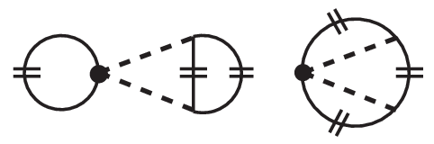
We continue with the three-body contributions from the -exchange Hartree diagram shown in the left part of Fig. 2. Again putting in three medium insertions one derives the following analytical results:
| (20) | |||||
| (21) |
| (22) |
which depend only on the two isoscalar coupling constants and . The isovectorial (spin-dependent) -vertex gets eliminated by a vanishing spin-trace (over the left nucleon ring). The vanishing contributions to and from the -exchange three-body Hartree diagram are particularly remarkable, in view of the fact that their isoscalar counterparts ( and in eqs.(24,25) of ref.[13]) are quite sizeable. The actual calculation shows that the isospin-structure of the -vertex excludes the desired coupling of the gradient to the vectors and .
4.4 Fock diagram proportional to
Finally, there are the three-body contributions from the -exchange Fock diagram shown in the right part of Fig. 2. For this diagram the occurring integrals over three Fermi spheres cannot be solved analytically in all cases. After a somewhat tedious calculation of the separate pieces proportional to , and one finds the following results for the Fock contributions to the strength functions:
| (23) | |||||
with the auxiliary functions:
| (24) |
| (25) | |||||
| (26) | |||||
A double-index notation has been introduced for partial derivatives multiplied by powers of the variables and :
| (27) |
which applies in the same way to the functions and .
| (28) | |||||
with the auxiliary function:
| (29) |
| (30) | |||||
| (31) | |||||
| (32) | |||||
with given in eq.(29). A good check of all formulas collected in this section is provided by their Taylor-expansion in . Despite the superficial opposite appearance the leading term in the -expansion is . In several cases it is even a higher power of . The full Taylor series in has however a small radius of convergence , corresponding to tiny densities fm-3. Let us also take the occasion to correct the expression for written in eq.(27) of ref.[19]. The correct expression is obtained by inserting into eq.(31) the parameters , and . The term omitted in ref.[19] vanishes (accidentally) for the original density-matrix expansion of Negele and Vautherin [9] but not for the improved density-matrix expansion of Gebremariam, Duguet and Bogner [10]. The numerical consequences of this correction are insignificant since (at half nuclear matter density fm-3) the already small contribution MeVfm5 gets just further reduced to MeVfm5.
5 Results and discussion
In this section we present and discuss our numerical results obtained by summing the series of two- and three-body contributions given in sections 3 and 4. The physical input parameters are: (nucleon axial vector coupling constant), MeV (pion decay constant) and MeV (average pion mass). We use consistently the same parameters pertinent to the chiral three-nucleon interaction: , , MeV, GeV-1, GeV-1 and GeV-1, as in our previous work [13] on the isoscalar part of the nuclear energy density functional. Let us remind that the low-energy constants and have been obtained in refs.[15, 16] by fitting them simultaneously (after fixing MeV) to the binding energies of 3H and 4He using the low-momentum NN-interaction [7] at a cutoff scale of MeV.

Fig. 3 shows the contributions to the asymmetry energy of infinite spin-saturated nuclear matter for densities up to fm-3. The dash-dotted and dashed line give the two-body and three-body contributions to this quantity. Their sum, the total interaction contribution, is shown by the full line in Fig. 3. In the Hartree-Fock approximation the asymmetry energy is completed by adding the (relativistically improved) kinetic energy contribution , with MeV the (free) nucleon mass. Adding these three pieces together, one obtains for the asymmetry energy at nuclear matter saturation density fm-3 the value MeV. This is compatible with the empirical values MeV extracted in extensive fits of nuclide masses in refs.[20, 21]. For comparison, a recent microscopic estimate of the asymmetry energy in a relativistic mean-field model (constrained by some specific properties of certain nuclei) gave the value MeV [22]. Note that about 1/3 of the empirical value is provided by the kinetic energy: MeV. Another quantity of interest is the slope of the asymmetry energy at saturation density. We find for the slope parameter MeV which is again compatible with the value MeV quoted in ref.[21]. It is remarkable that the Hartree-Fock approximation works already reasonably well for the asymmetry energy when giving results that are about smaller than empirical determinations. In contrast to this, the Hartree-Fock approximation gives a much too shallow binding minimum in the equation of state of isospin-symmetric nuclear matter (see Fig. 7 in ref.[13]), and second order corrections are very important in order to converge eventually to the empirical saturation point [15, 23]. The role of three-nucleon forces is also different for both quantities. On the one hand side repulsive three-body effects are essential in order to achieve saturation of nuclear matter but they do contribute little to the asymmetry energy , in the present calculation merely MeV. It is also interesting to remind that the one-pion exchange alone produces a negative contribution to the asymmetry energy:
| (33) |
which amounts to MeV at normal nuclear matter density fm-3.

Fig. 4 shows the contributions to the strength function . One observes that the (negative) two-body contributions get somewhat reduced in size by the (positive) three-body corrections. For orientation we have included in Fig. 4 also the one-pion exchange contribution to as given by the expression:
| (34) |
with . One recognizes that this relatively small contribution becomes almost independent of density for fm-3. Note that according its construction the term in the nuclear energy density functional eq.(2) splits the effective (in-medium) masses of protons and neutrons in linear proportion to a (local) isospin-asymmetry . By comparison with the isoscalar strength function (see Fig. 8 in ref.[13]) one concludes that the isovector strength function is suppressed by about a factor 5 and of opposite sign.
Next, we show in Fig. 5 the strength function of the isovector surface term . The three-body contribution to this quantity is negligible. Furthermore, one observes from Fig. 5 that both components and (see eq.(3)) are of equal importance for the strength function . The pronounced decrease at very low densities fm-3 is caused by the -exchange and has also been observed in other calculations [11]. In phenomenological Skyrme parameterizations the strength function is a constant, whose value is however not well determined. Taking the modern Sly forces [3] as a guideline one obtains the band MeVfm5 which covers well the results of present (microscopic) calculation. For comparison the strength function of the isoscalar surface term is about one order of magnitude larger and empirically much better determined: MeVfm5 [3].


Next, we show in Fig. 6 the strength function of the isovector spin-orbit coupling term . One sees that the weak decrease of the two-body contribution with density gets compensated by a small (positive) three-body contribution. The resulting total spin-orbit coupling strength comes out close to the constant value MeVfm5 of Skyrme parameterizations [3, 4]. At this point it should be emphasized that the isovector spin-orbit coupling strength in nuclei is presently not well determined. For example, no definite choice could be made in ref.[24] between different density-dependences of the neutron spin-orbit potential.
Finally, we show in Fig. 7 the strength function accompanying the squared isovector spin-orbit density in the nuclear energy density functional. The two-body and three-body contributions come with equal sign but exhibit an opposite density-dependence. For orientation we have included in Fig. 7 also the one-pion exchange contribution to as given by the expression:
| (35) |
Apparently, the strength function is dominated by this unique long-range contribution which is also responsible for the strong density-dependence [11] below fm-3. At this point it should be kept in mind that the term in the nuclear energy density functional eq.(2) represents non-local Fock contributions from tensor forces etc. An outstanding -exchange contribution to is therefore not surprising.
In summary we have calculated the strength functions of isovector terms in the nuclear energy density functional from chiral two-and three-nucleon interactions. The results for asymmetry energy suggest that the Hartree-Fock approximation could work better for isovector quantities. Clearly, it remains a challenge to confirm this in a consistent second-order calculation of the complete nuclear energy density functional.
Acknowledgement
I thank J.W. Holt for providing the N3LOW chiral NN-potential in parameterized numerical form and for informative discussions.
References
- [1] M. Bender, P.H. Heenen and P.G. Reinhard, Rev. Mod. Phys. 75 (2003) 121.
- [2] J.R. Stone and P.G. Reinhard, Prog. Part. Nucl. Phys. 58 (2007) 587.
- [3] E. Chabanat, E. Bonche, P. Haensel, J. Meyer and P. Schaeffer, A635 (1998) 231.
- [4] N. Chamel, S. Goriely and J.M. Pearson, Nucl. Phys. A812 (2008) 72.
- [5] B.D. Serot and J.D. Walecka, Int. J. Mod. Phys. E6 (1997) 515.
- [6] T. Niksic, D. Vretenar and P. Ring, Prog. Part. Nucl. Phys. 66 (2011) 519.
- [7] S.K. Bogner, R.J. Furnstahl and A. Schwenk, Prog. Part. Nucl. Phys. 65 (2010) 94.
- [8] S.K. Bogner, T.T.S. Kuo and A. Schwenk, Phys. Reports 386 (2003) 1.
- [9] J.W. Negele and D. Vautherin, Phys. Rev. C5 (1972) 1472.
- [10] B. Gebremariam, T. Duguet and S.K. Bogner, Phys. Rev. C82 (2010) 014305.
- [11] B. Gebremariam, S.K. Bogner and T. Duguet, Nucl. Phys. A851 (2011) 17.
- [12] M. Stoitsov et al., Phys. Rev. C82 (2010) 054307.
- [13] N. Kaiser, J.W. Holt and W. Weise, Eur. Phys. A47 (2011) 128.
- [14] L. Coraggio et al., Phys. Rev. C75 (2007) 024311.
- [15] S.K. Bogner, R.J. Furnstahl, A. Nogga and A. Schwenk, Nucl. Phys. A763 (2005) 59.
- [16] A. Nogga, S.K. Bogner and A. Schwenk, Phys. Rev. C70 (2004) 061002.
- [17] E. Epelbaum, W. Glöckle and Ulf-G. Meißner, Nucl. Phys. A747 (2005) 362.
- [18] S.K. Bogner, R.J. Furnstahl and L. Platter, Eur. Phys. J. A39 (2009) 219.
- [19] N. Kaiser, Eur. Phys. A45 (2010) 61.
- [20] P.A. Seeger and W.M. Howard, Nucl. Phys. A238 (1975) 491.
- [21] J.P. Blaizot, Phys. Reports 64 (1980) 171.
- [22] D. Vretenar, T. Niksic and P. Ring, Phys. Rev. C68 (2003) 024310.
- [23] K. Hebeler et al, Phys. Rev. C83 (2011) 031301.
- [24] P.G. Reinhard and H. Flocard, Nucl. Phys. A584 (1995) 467.