Inclusive Hadron Productions in $pA$ Collisions

Giovanni A. Chirilli Affiliation: Nuclear Science Division, Lawrence Berkeley National Laboratory, Berkeley, CA 94720, USA Bo-Wen Xiao Affiliation: Department of Physics, Pennsylvania State University, University Park, PA 16802, USA Feng Yuan Affiliation: Nuclear Science Division, Lawrence Berkeley National Laboratory, Berkeley, CA 94720, USA

Abstract

We calculate inclusive hadrons production in $pA$ collisions in the small- $x$ saturation formalism at one-loop order. The differential cross section is written into a factorization form in the coordinate space at the next-to-leading order, while the naive form of the convolution in the transverse momentum space does not hold. The rapidity divergence with small- $x$ dipole gluon distribution of the nucleus is factorized into the energy evolution of the dipole gluon distribution function, which is known as the Balitsky-Kovchegov equation. Furthermore, the collinear divergences associated with the incoming parton distribution of the nucleon and the outgoing fragmentation function of the final state hadron are factorized into the splittings of the associated parton distribution and fragmentation functions, which allows us to reproduce the well-known DGLAP equation. The hard coefficient function, which is finite and free of divergence of any kind, is evaluated at one-loop order.

I Introduction

Inclusive hadron production in $pA$ collisions have attracted much of theoretical interests in recent years [1, 2, 3, 4, 6, 5, 7, 8, 9, 10, 11, 12, 13]. In particular, the suppression of hadron production in the forward $dAu$ scattering at RHIC observed in the experiments [14, 15] has been regarded as one of the evidences for the gluon saturation at small- $x$ in a large nucleus [7, 8, 16]. Saturation phenomenon at small- $x$ in nucleon and nucleus plays an important role in high energy hadronic scattering [17, 18, 19, 20]. In this paper, as an important step toward a complete description of hadron production in $pA$ collisions in the saturation formalism, we calculate the one-loop perturbative corrections. Previous attempts have been made in the literature. In particular, in Ref. [5], part of one-loop diagrams were evaluated. However, the rapidity divergence is not identified and the collinear evolution effects are not complete. Recently, some of the higher order corrections were discussed in Ref. [9], where it was referred as “inelastic” contribution. In the following, we will calculate the complete next-to-leading order (NLO) corrections to this process in the saturation formalism. A brief summary of our results has been published earlier in Ref. [21].

Inclusive hadron production in $pA$ collisions,

p+A\to h+X\ ,

(1)

can be viewed as a process where a parton from the nucleon (with momentum $p$ ) scatters on the nucleus target (with momentum $P_{A}$ ), and fragments into final state hadron with momentum $P_{h}$ . In the dense medium of the large nucleus and at small- $x$ , the multiple interactions become important, and we need to perform the relevant resummation to make the reliable predictions. This is particularly important because the final state parton is a colored object. Its interactions with the nucleus target before it fragments into the hadron is crucial to understand the nuclear effects in this process. In our calculations, we follow the high energy factorization, also called color-dipole or color-glass-condensate (CGC), formalism [22, 23, 20] to evaluate the above process up to one-loop order. We notice that alternative approaches have been proposed in the literature [10, 11, 12, 13] to calculate the nuclear effects in this process.

According to our calculations, the QCD factorization formalism for the above process reads as,

\displaystyle\frac{d^{3}\sigma^{p+A\to h+X}}{dyd^{2}p_{\perp}}

\displaystyle=

\displaystyle\sum\limits_{a}\int\frac{dz}{z^{2}}\frac{dx}{x}\xi xf_{a}(x,\mu)D_{h/c}(z,\mu)\int[dx_{\perp}]S_{a,c}^{Y}([x_{\perp}])\mathcal{H}_{a\to c}(\alpha_{s},\xi,[x_{\perp}]\mu)\ ,

(2)

where $\xi=\tau/xz$ with $\tau=p_{\perp}e^{y}/\sqrt{s}$ , $y$ and $p_{\perp}$ the rapidity and transverse momentum for the final state hadron and $s$ the total center of mass energy square $s=(p+P_{A})^{2}$ , respectively. Schematically, this factorization is illustrated in Fig. 1, where the incoming parton described by the parton distribution $f_{a}(x)$ scatters off the nuclear target represented by multiple-point correlation function $S^{Y}([x_{\perp}])$ , and fragments into the final state hadron defined by the fragmentation function $D_{h/c}(z)$ . All these quantities have clear operator definitions in QCD. In particular, $f_{a}(x)$ and $D_{h/c}(z)$ are collinear parton distribution and fragmentation functions which only depend on the longitudinal momentum fraction $x$ of the nucleon carried by the parton $a$ , and the momentum fraction $z$ of parton $c$ carried by the final state hadron $h$ , respectively. From the nucleus side, it is the multi-point correlation functions denoted as $S_{a,c}^{Y}(x_{\perp})$ (see the definitions below) that enters in the factorization formula, depending on the flavor of the incoming and outgoing partons and the gluon rapidity $Y$ associated with the nucleus: $Y\approx\ln(1/x_{g})$ with $x_{g}$ being longitudinal momentum fraction.

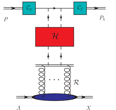
Refer to caption — Figure 1: Schematic plot of the factorization, where $\mathcal{H}$ indicates the hard factor, $\mathcal{R}$ represents the rapidity divergence which are factorized into the dipole gluon distribution of the target nucleus ( $A$ ), $\mathcal{C}_{p}$ and $\mathcal{C}_{f}$ stand for the collinear divergences which are absorbed into the parton distribution functions of the projectile proton ( $P$ ) and hadron ( $P_{h}$ ) fragmentation functions, respectively.

At the leading order, $S^{Y}$ represent the two-point functions, including the dipole gluon distribution functions in the elementary and adjoint representations for the quark and gluon initialed subprocesses [20], respectively. Higher order corrections will have terms that depend on the correlation functions beyond the simple two-point functions. Because of this reason, the integral $[dx_{\perp}]$ represents all possible integrals at the particular order.

To evaluate NLO corrections, we will calculate the gluon radiation contributions. At one-loop order, the gluon radiation will introduce various divergences. The factorization formula in Eq. (2) is to factorize these divergences into the relevant factors. For example, there will be collinear divergences associated with the incoming parton distribution and final state fragmentation functions. In addition, there is the rapidity divergence associated with $S^{Y}([x_{\perp}])$ . These divergences naturally show up in higher order calculations. The idea of the factorization is to demonstrate that these divergences can be absorbed into the various factors in the factorization formula. After subtracting these divergences, we will obtain the hard factors $\mathcal{H}_{a\to c}$ , which describes the partonic scattering amplitude of parton $a$ into a parton $c$ in the dense medium. This hard factor includes all order perturbative corrections, and can be calculated order by order. Although there is no simple $k_{\perp}$ -factorization form beyond leading order formalism, we will find that in the coordinate space, the cross section can be written into a nice factorization form as Eq. (2). Besides the explicit dependence on the variables shown in Eq. (2), there are implicit dependences on $p_{\perp}[x_{\perp}]$ in the hard coefficients as well.

Two important variables are introduced to separate different factorizations for the physics involved in this process: the collinear factorization scale $\mu$ and the energy evolution rapidity dependence $Y$ . The physics associated with $\mu$ follows the normal collinear QCD factorization, whereas the rapidity factorization $Y$ takes into account the small- $x$ factorization. The evolution respect to $\mu$ is controlled by the usual DGLAP evolution, whereas that for $S_{a}^{Y}$ by the Balitsky-Kovchegov (BK) evolution [23, 24]. In general, the energy evolution of any correlation functions can be given by the JIMWLK equation[25], and the resulting equation is equivalent to the BK equation for dipole amplitudes. In particular, our one-loop calculations will demonstrate the important contribution from this rapidity divergence. Schematically, this factorization is shown in Fig. 1.

Our calculations should be compared to the similar calculations at next-to-leading order for the DIS structure functions in the saturation formalism [26, 27, 28]. All these calculations are important steps to demonstrate the factorization for general hard processes in the small- $x$ saturation formalism [29]. The rest of the paper is organized as follows. In Sec. II, we discuss the leading order results for inclusive hadron production in $pA$ collision, where we also set up the framework for the NLO calculations. Sec. III. is divided into four subsections, in which we calculate the NLO cross section for the $q\to q$ , $g\to g$ , $q\to g$ and $g\to q$ channels . The summary and further discussions are given in Sec. IV.

II The leading order single inclusive cross section.

The leading order result was first formulated in Ref. [1]. For the purpose of completeness, we briefly derive the leading order cross section to set up the baseline for the NLO calculation. Let us begin with the quark channel in $pA$ collisions. As illustrated in Fig. 2, the multiple scattering between the quark from the proton and the dense gluons inside the nucleus target can be cast into the Wilson line

U(x_{\perp})=\mathcal{P}\exp\left\{ig_{S}\int_{-\infty}^{+\infty}\text{d}x^{+}\,T^{c}A_{c}^{-}(x^{+},x_{\perp})\right\}\ ,

(3)

with $A_{c}^{-}(x^{+},x_{\perp})$ being the gluon field solution of the classical Yang-Mills equation inside the large nucleus target.

Therefore, the leading-order cross section for producing a quark with finite transverse momentum $k_{\perp}$ at rapidity $y$ in the channel $qA\rightarrow qX$ can be written as:

\frac{d\sigma_{\text{LO}}^{pA\rightarrow qX}}{d^{2}k_{\perp}dy}=\sum_{f}xq_{f}(x)\int\frac{d^{2}x_{\perp}d^{2}y_{\perp}}{(2\pi)^{2}}e^{-ik_{\perp}\cdot(x_{\perp}-y_{\perp})}\frac{1}{N_{c}}\left\langle\text{Tr}U(x_{\perp})U^{\dagger}(y_{\perp})\right\rangle_{Y},

(4)

with $x=\frac{k_{\perp}}{\sqrt{s}}e^{y}$ and $x_{g}=\frac{k_{\perp}}{\sqrt{s}}e^{-y}$ . The notation $\langle\dots\rangle_{Y}$ indicates the CGC average of the color charges over the nuclear wave function where $Y\simeq\ln 1/x_{g}$ and $x_{g}$ is the smallest longitudinal momentum fraction of the probed gluons, and is determined by the kinematics ¹¹ 1 Here we are only interested in the inelastic production of the quark in the forward scattering which produces quark with finite transverse momentum. There is also elastic scattering contribution to the cross section which generates vanishing $k_{\perp}$ , such as $\sum_{f}xq_{f}(x)\delta^{(2)}(k_{\perp})\int d^{2}b$ to the total cross section.. Normally, we first compute the correlator $\left\langle\text{Tr}U(x_{\perp})U^{\dagger}(y_{\perp})\right\rangle$ in the McLerran-Venugopalan model[19] as the initial condition, and then we perform the energy evolution for the correlator which introduces the rapidity ( $Y$ ) dependence. The energy evolution equation at small- $x$ for dense nucleus targets is the BK equation as we shall demonstrate later when we remove the rapidity divergence. When multiplied by the fragmentation function, the above result will lead to the differential cross section for hadron production in $pA$ collisions.

It is straightforward to include the gluon initiated channel, and the full leading order hadron production cross section can be written as

\frac{d\sigma_{\text{LO}}^{pA\rightarrow hX}}{d^{2}p_{\perp}dy_{h}}=\int_{\tau}^{1}\frac{dz}{z^{2}}\left[\sum_{f}x_{p}q_{f}(x_{p})\mathcal{F}(k_{\perp})D_{h/q}(z)+x_{p}g(x_{p})\tilde{\mathcal{F}}(k_{\perp})D_{h/g}(z)\right],

(5)

with $p_{\perp}=zk_{\perp}$ , $x_{p}=\frac{p_{\perp}}{z\sqrt{s}}e^{y_{h}}$ , $\tau=zx_{p}$ and $x_{g}=\frac{p_{\perp}}{z\sqrt{s}}e^{-y_{h}}$ . Here we have defined

\mathcal{F}(k_{\perp})=\int\frac{d^{2}x_{\perp}d^{2}y_{\perp}}{(2\pi)^{2}}e^{-ik_{\perp}\cdot(x_{\perp}-y_{\perp})}S_{Y}^{(2)}(x_{\perp},y_{\perp}),

(6)

with $S_{Y}^{(2)}(x_{\perp},y_{\perp})=\frac{1}{N_{c}}\left\langle\text{Tr}U(x_{\perp})U^{\dagger}(y_{\perp})\right\rangle_{Y}$ . $\tilde{\mathcal{F}}(k_{\perp})$ is defined similarly but in the adjoint representation

\tilde{\mathcal{F}}(k_{\perp})=\int\frac{d^{2}x_{\perp}d^{2}y_{\perp}}{(2\pi)^{2}}e^{-ik_{\perp}\cdot(x_{\perp}-y_{\perp})}\tilde{S}_{Y}^{(2)}(x_{\perp},y_{\perp}),

(7)

where $\tilde{S}_{Y}^{(2)}(x_{\perp},y_{\perp})=\frac{1}{N_{c}^{2}-1}\left\langle\text{Tr}W(x_{\perp})W^{\dagger}(y_{\perp})\right\rangle_{Y}$ and $W(x)$ is a Wilson line in the adjoint representation. It represents the multiple interaction between the final state gluon and the nucleus target. In general, the adjoint Wilson lines can be replaced by two fundamental Wilson lines by using the identity

W^{ab}(x_{\perp})=2\text{Tr}\left[T^{a}U(x_{\perp})T^{b}U^{\dagger}(x_{\perp})\right],

(8)

and the color matrices can be removed using the Fierz identity $T^{a}_{ij}T^{a}_{kl}=\frac{1}{2}\delta_{il}\delta_{jk}-\frac{1}{2N_{c}}\delta_{ij}\delta_{kl}$ . It is straightforward to show that

\tilde{S}_{Y}^{(2)}(x_{\perp},y_{\perp})=\frac{1}{N_{c}^{2}-1}\left[\left\langle\text{Tr}U(x_{\perp})U^{\dagger}(y_{\perp})\textrm{Tr}U(y_{\perp})U^{\dagger}(x_{\perp})\right\rangle_{Y}-1\right],

(9)

which, in the large $N_{c}$ limit, allows us to write

\tilde{\mathcal{F}}(k_{\perp})=\int\frac{d^{2}x_{\perp}d^{2}y_{\perp}}{(2\pi)^{2}}e^{-ik_{\perp}\cdot(x_{\perp}-y_{\perp})}S_{Y}^{(2)}(x_{\perp},y_{\perp})S_{Y}^{(2)}(y_{\perp},x_{\perp})\ .

(10)

It is very important to keep in mind that the normalization of the dipole amplitudes $S^{(2)}(x_{\perp},y_{\perp})$ is unity when $x_{\perp}=y_{\perp}$ . In addition, since normally $\left\langle\text{Tr}U(x_{\perp})U^{\dagger}(y_{\perp})\right\rangle_{Y}$ is real, it is easy to see that $S^{(2)}(x_{\perp},y_{\perp})=S^{(2)}(y_{\perp},x_{\perp})$ . If we further neglect the impact parameter dependence, one will find that $S^{(2)}(x_{\perp},y_{\perp})=\exp\left[-\frac{Q_{s}^{2}(x_{\perp}-y_{\perp})^{2}}{4}\right]$ in the McLerran-Venugopalan model, where $Q_{s}$ is the saturation momentum which characterizes the density of the target nucleus. The analytical form of the dipole amplitude can help us to test the properties of dipole amplitudes mentioned above.

We would like to emphasize that in Eq. (5) we do not include the transverse momentum dependence in the incoming parton distribution from the nucleon. In the forward $pA$ collisions, the transverse momentum dependence from the incoming parton distribution of the nucleon is not as important as that from the nucleus target. Therefore, in the current calculations, we neglect this effect. As a consistent check, the one-loop calculations in the following support this assumption. In particular, the collinear divergence associated with the incoming parton distribution contains no transverse momentum dependence.

III The Next-to-leading order cross section

In this section, we will present the detailed calculations for the NLO corrections to the leading order result in Eq. (5). There are four partonic channels: $q\to qg$ , $g\to gg$ , $q\to gq$ , $g\to q\bar{q}$ . We will carry out the calculations for these channels separately.

III.1 The quark channel $q\to q$

The quark production contribution contains the real and virtual gluon radiation at the NLO. For the real contribution, we will calculate $q\rightarrow qg$ first. The real diagrams with a quark (with transverse coordinate $b_{\perp}$ ) and gluon (with transverse coordinate $x_{\perp}$ ) in the final state, as shown in Fig. 3, have been studied in Ref. [30, 31, 32]. We take eq.(78) of Ref. [32] as our starting point which gives²² 2 For convention reasons, we have interchanged the definition of $z$ and $1-z$ and replaced the variable $z$ by $\xi$ .

$\displaystyle\frac{d\sigma^{qA\rightarrow qgX}}{d^{3}k_{1}d^{3}k_{2}}$	$\displaystyle=$	$\displaystyle\alpha_{S}C_{F}\delta(p^{+}-k_{1}^{+}-k_{2}^{+})\int\frac{\text{d}^{2}x_{\perp}}{(2\pi)^{2}}\frac{\text{d}^{2}x_{\perp}^{\prime}}{(2\pi)^{2}}\frac{\text{d}^{2}b_{\perp}}{(2\pi)^{2}}\frac{\text{d}^{2}b_{\perp}^{\prime}}{(2\pi)^{2}}$	(11)
		$\displaystyle\times e^{-ik_{1\perp}\cdot(x_{\perp}-x^{\prime}_{\perp})}e^{-ik_{2\perp}\cdot(b_{\perp}-b_{\perp}^{\prime})}\sum_{\lambda\alpha\beta}\psi^{\lambda\ast}_{\alpha\beta}(u^{\prime}_{\perp})\psi^{\lambda}_{\alpha\beta}(u_{\perp})$
		$\displaystyle\times\left[S^{(6)}_{Y}(b_{\perp},x_{\perp},b^{\prime}_{\perp},x^{\prime}_{\perp})+S^{(2)}_{Y}(v_{\perp},v^{\prime}_{\perp})\right.$
		$\displaystyle\quad\left.-S^{(3)}_{Y}(b_{\perp},x_{\perp},v^{\prime}_{\perp})-S^{(3)}_{Y}(v_{\perp},x^{\prime}_{\perp},b^{\prime}_{\perp})\right].$

where $u_{\perp}=x_{\perp}-b_{\perp}$ , $u^{\prime}_{\perp}=x^{\prime}_{\perp}-b^{\prime}_{\perp}$ , $v_{\perp}=(1-\xi)x_{\perp}+\xi b_{\perp}$ , $v^{\prime}_{\perp}=(1-\xi)x^{\prime}_{\perp}+\xi b^{\prime}_{\perp}$ and

	$\displaystyle S^{(6)}_{Y}(b_{\perp},x_{\perp},b^{\prime}_{\perp},x^{\prime}_{\perp})$	$\displaystyle=\frac{1}{C_{F}N_{c}}\left\langle\text{Tr}\left(U(b_{\perp})U^{\dagger}(b^{\prime}_{\perp})T^{d}T^{c}\right)\left[W(x_{\perp})W^{\dagger}(x^{\prime}_{\perp})\right]^{cd}\right\rangle_{Y},$		(12)
	$\displaystyle S^{(3)}_{Y}(b_{\perp},x_{\perp},v^{\prime}_{\perp})$	$\displaystyle=\frac{1}{C_{F}N_{c}}\left\langle\text{Tr}\left(U(b_{\perp})T^{d}U^{\dagger}(v^{\prime}_{\perp})T^{c}\right)W^{cd}(x_{\perp})\right\rangle_{Y}.$		(13)

For a right-moving massless quark, with initial longitudinal momentum $p^{+}$ and no transverse momentum, the splitting wave function in transverse coordinate space is given by

\psi^{\lambda}_{\alpha\beta}(p^{+},k_{1}^{+},r_{\perp})=2\pi i\sqrt{\frac{2}{k_{1}^{+}}}\begin{cases}\frac{r_{\perp}\cdot\epsilon^{(1)}_{\perp}}{r_{\perp}^{2}}(\delta_{\alpha-}\delta_{\beta-}+\xi\delta_{\alpha+}\delta_{\beta+}),&\lambda=1,\\ \frac{r_{\perp}\cdot\epsilon^{(2)}_{\perp}}{r_{\perp}^{2}}(\delta_{\alpha+}\delta_{\beta+}+\xi\delta_{\alpha-}\delta_{\beta-}),&\lambda=2.\end{cases}\ ,

(14)

where $\lambda$ is the gluon polarization, $\alpha,\beta$ are helicities for the incoming and outgoing quarks, and $1-\xi=\frac{k_{1}^{+}}{p^{+}}$ is the momentum fraction of the incoming quark carried by the gluon. Since the Wilson lines in the fundamental representation and the adjoint representation resum the multiple interactions of quarks and gluons with the nucleus target, respectively, one can easily see that these four terms in the last two lines of the Eq. (11) correspond to those four graphs in Fig. 3. The $S^{(6)}_{Y}$ term which corresponds to Fig. 3 (a) and resums all the multiple interactions between the quark-gluon pair and the nucleus target, represents the case where interactions take place after the splitting both in the amplitude and in the conjugate amplitude. The $S^{(2)}_{Y}$ term which comes from Fig. 3 (b), resums the interactions before the splitting only and the $S^{(3)}_{Y}$ terms represent the interference terms as shown in Fig. 3 (c) and (d).

There are two contributions for inclusive hadron production at the next-to-leading order, namely, quark productions associated with $D_{h/q}$ which is indicated by the cross in Fig. 3 (while the gluon is integrated) and gluon productions associated with the fragmentation function $D_{h/g}$ (while the quark is integrated).

Let us study the former case by integrating over the phase space of the final state gluon $(k^{+}_{1},k_{1\perp})$ . We can cast the real contribution into

	$\displaystyle\frac{\alpha_{s}}{2\pi^{2}}\int\frac{dz}{z^{2}}D_{h/q}(z)\int_{\tau/z}^{1}d\xi\frac{1+\xi^{2}}{1-\xi}xq(x)\left\{C_{F}\int d^{2}k_{g\perp}\mathcal{I}(k_{\perp},k_{g\perp})\right.$
	$\displaystyle\left.~~~+\frac{N_{c}}{2}\int d^{2}k_{g\perp}d^{2}{k_{g1\perp}}\mathcal{J}(k_{\perp},k_{g\perp},k_{g1\perp})\right\}\ ,$		(15)

where $x=\tau/z\xi$ and $C_{F}=(N_{c}^{2}-1)/2N_{c}$ , and $\mathcal{I}$ and $\mathcal{J}$ are defined as

$\displaystyle\mathcal{I}(k_{\perp},k_{g\perp})$	$\displaystyle=$	$\displaystyle\mathcal{F}(k_{g\perp})\left[\frac{k_{\perp}-k_{g\perp}}{(k_{\perp}-k_{g\perp})^{2}}-\frac{k_{\perp}-\xi k_{g\perp}}{(k_{\perp}-\xi k_{g\perp})^{2}}\right]^{2},$
$\displaystyle\mathcal{J}(k_{\perp},k_{g\perp},k_{g1\perp})$	$\displaystyle=$	$\displaystyle\left[\mathcal{F}(k_{g\perp})\delta^{\left(2\right)}\left(k_{g1\perp}-k_{g\perp}\right)-\mathcal{G}(k_{g\perp},k_{g1\perp})\right]\frac{2(k_{\perp}-\xi k_{g\perp})\cdot(k_{\perp}-k_{g1\perp})}{(k_{\perp}-\xi k_{g\perp})^{2}(k_{\perp}-k_{g1\perp})^{2}}\ ,$
$\displaystyle\text{with}\quad\mathcal{G}(k_{\perp},l_{\perp})$	$\displaystyle=$	$\displaystyle\int\frac{d^{2}x_{\perp}d^{2}y_{\perp}d^{2}b_{\perp}}{(2\pi)^{4}}e^{-ik_{\perp}\cdot(x_{\perp}-b_{\perp})-il_{\perp}\cdot(b_{\perp}-y_{\perp})}S_{Y}^{(4)}(x_{\perp},b_{\perp},y_{\perp}),$	(16)

and $S_{Y}^{(4)}(x_{\perp},b_{\perp},y_{\perp})=\frac{1}{N_{c}^{2}}\langle\mathrm{Tr}[{U}(x_{\perp}){U}^{\dagger}(b_{\perp})]\mathrm{Tr}[{U}(b_{\perp}){U}^{\dagger}(y_{\perp})]\rangle_{Y}$ . Several steps are necessary in deriving the above result from Eq. (11). By integrating over the gluon momentum, we identify $x_{\perp}$ to $x^{\prime}_{\perp}$ which simplifies $S^{(6)}_{Y}$ to $S^{(2)}(b_{\perp},b^{\prime}_{\perp})$ . This is expected since we know the multiple interactions between the gluon and the nucleus target should cancel if the gluon is not observed. Furthermore, using the Fierz identity, one can write

S^{(3)}_{Y}(b_{\perp},x_{\perp},v^{\prime}_{\perp})=\frac{N_{c}}{2C_{F}}\left[S_{Y}^{(4)}(b_{\perp},x_{\perp},v^{\prime}_{\perp})-\frac{1}{N_{c}^{2}}S_{Y}^{(2)}(b_{\perp},v^{\prime}_{\perp})\right],

(17)

which only involves the Wilson lines in the fundamental representation. Then, the final steps, which include the Fourier transforms, as well as the convolutions of the quark distribution and fragmentation function, are quite straightforward.

Before we proceed to the calculations of the virtual diagrams, we comment on the result shown in Eq. (15). The major obstacles of evaluating the integrals in Eq. (15) are the divergences. There are three types of singularities lying in that equation, namely, the rapidity divergence which occurs at $\xi=1$ when the rapidity of the radiated gluon becomes $-\infty$ , and the collinear singularities which correspond to the cases that the final state gluon is either collinear to the initial quark or final state quark. We shall expect that the virtual diagrams cancel some part of the divergences, while the uncancelled divergences shall be absorbed into the renormalization of the quark distribution and fragmentation functions as well as the target dipole gluon distribution ( $S_{Y}^{(2)}(x_{\perp},y_{\perp})$ ). After these subtractions, the remainder contributions should be finite and give us the NLO correction to the single inclusive hadron production cross section.

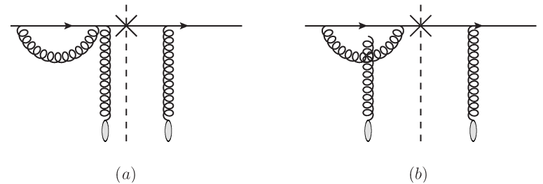
The evaluation of the virtual graphs as shown in Fig. 4 are quite simple in the dipole picture. Their contributions are proportional to

	$\displaystyle-2\alpha_{s}C_{F}\int\frac{d^{2}v_{\perp}}{(2\pi)^{2}}\frac{d^{2}v^{\prime}_{\perp}}{(2\pi)^{2}}\frac{d^{2}u_{\perp}}{(2\pi)^{2}}e^{-ik_{\perp}\cdot(v_{\perp}-v^{\prime}_{\perp})}\sum_{\lambda\alpha\beta}\psi^{\lambda\ast}_{\alpha\beta}(u_{\perp})\psi^{\lambda}_{\alpha\beta}(u_{\perp})$
	$\displaystyle\times\left[S_{Y}^{(2)}(v_{\perp},v_{\perp}^{\prime})-S^{(3)}_{Y}(b_{\perp},x_{\perp},v^{\prime}_{\perp})\right],$		(18)

where the factor of $2$ takes care of the fact that the mirror diagrams of Fig. 4 give the identical contributions when the virtual loop is on the right side of the cut. It is straightforward to see that these two terms in the last line of Eq. (18) correspond to the Fig. 4 (a) and (b), respectively. This eventually leads to

	$\displaystyle-\frac{\alpha_{s}}{2\pi^{2}}\int\frac{dz}{z^{2}}D_{h/q}(z)x_{p}q(x_{p})\int_{0}^{1}d\xi\frac{1+\xi^{2}}{1-\xi}$
	$\displaystyle\times\left\{C_{F}\int d^{2}q_{\perp}\mathcal{I}(q_{\perp},k_{\perp})+\frac{N_{c}}{2}\int d^{2}q_{\perp}d^{2}{k_{g1\perp}}\mathcal{J}(q_{\perp},k_{\perp},k_{g1\perp})\right\}\ ,$		(19)

where explicitly one writes

	$\displaystyle\mathcal{I}(q_{\perp},k_{\perp})$	$\displaystyle=$	$\displaystyle\mathcal{F}(k_{\perp})\left[\frac{q_{\perp}-k_{\perp}}{(q_{\perp}-k_{\perp})^{2}}-\frac{q_{\perp}-\xi k_{\perp}}{(q_{\perp}-\xi k_{\perp})^{2}}\right]^{2},$
	$\displaystyle\mathcal{J}(q_{\perp},k_{\perp},k_{g1\perp})$	$\displaystyle=$	$\displaystyle\left[\mathcal{F}(k_{\perp})\delta^{\left(2\right)}\left(k_{g1\perp}-k_{\perp}\right)-\mathcal{G}(k_{\perp},k_{g1\perp})\right]\frac{2(q_{\perp}-\xi k_{\perp})\cdot(q_{\perp}-k_{g1\perp})}{(q_{\perp}-\xi k_{\perp})^{2}(q_{\perp}-k_{g1\perp})^{2}}.$		(20)

It is easy to see that the virtual contributions indeed contain three types of singularities as we mentioned before. There are two important features that we wish to emphasize here. First, the rapidity divergence term is only proportional to $N_{c}/2$ since $\mathcal{I}$ vanishes at $\xi\to 1$ limit. This agrees with the BK equation since there is no $1/N_{c}^{2}$ corrections to the leading order BK equation. Second, when one integrates over the quark transverse momentum $k_{\perp}$ , the rapidity divergence disappears due to the complete cancellation between the real and virtual contributions.

III.1.1 The rapidity divergence

Now we are ready to evaluate NLO contributions by the following procedures. First, we remove the rapidity divergence terms from the real and virtual contributions by doing the following subtractions

	$\displaystyle\mathcal{F}(k_{\perp})$	$\displaystyle=$	$\displaystyle\mathcal{F}^{(0)}(k_{\perp})-\frac{\alpha_{s}N_{c}}{2\pi^{2}}\int_{0}^{1}\frac{d\xi}{1-\xi}\int\frac{d^{2}x_{\perp}d^{2}y_{\perp}d^{2}b_{\perp}}{(2\pi)^{2}}e^{-ik_{\perp}\cdot(x_{\perp}-y_{\perp})}$		(21)
			$\displaystyle\times\frac{(x_{\perp}-y_{\perp})^{2}}{(x_{\perp}-b_{\perp})^{2}(y_{\perp}-b_{\perp})^{2}}\left[S_{Y}^{(2)}(x_{\perp},y_{\perp})-S_{Y}^{(4)}(x_{\perp},b_{\perp},y_{\perp})\right]\ ,$		(21)

where $\mathcal{F}^{(0)}(k_{\perp})$ is the bare dipole gluon distribution which appears in the leading order cross section as in Eq. (5) and it is divergent. $\mathcal{F}(k_{\perp})$ is the renormalized dipole gluon distribution and it is assumed to be finite. We can always decompose the dipole splitting kernel as

\frac{(x_{\perp}-y_{\perp})^{2}}{(x_{\perp}-b_{\perp})^{2}(y_{\perp}-b_{\perp})^{2}}=\frac{1}{(x_{\perp}-b_{\perp})^{2}}+\frac{1}{(y_{\perp}-b_{\perp})^{2}}-\frac{2(x_{\perp}-b_{\perp})\cdot(y_{\perp}-b_{\perp})}{(x_{\perp}-b_{\perp})^{2}(y_{\perp}-b_{\perp})^{2}},

(22)

where the first two terms are removed from the virtual contribution while the last term is removed from the real diagrams. This procedure is similar to that for the collinear factorization, where we modify the bare leading order parton distributions to the finite parton distribution with the higher order radiation. Using Eqs. (6, 21), we can see that the differential change of the dipole amplitude $S_{Y}^{(2)}(x_{\perp},y_{\perp})$ yields the BK equation

\frac{\partial}{\partial Y}S_{Y}^{(2)}(x_{\perp},y_{\perp})=-\frac{\alpha_{s}N_{c}}{2\pi^{2}}\int\frac{d^{2}b_{\perp}\,(x_{\perp}-y_{\perp})^{2}}{(x_{\perp}-b_{\perp})^{2}(y_{\perp}-b_{\perp})^{2}}\left[S_{Y}^{(2)}(x_{\perp},y_{\perp})-S_{Y}^{(4)}(x_{\perp},b_{\perp},y_{\perp})\right]\ .

(23)

It is important to note that if we conduct the leading order classical calculation, we will not get any energy dependence, namely the $Y$ dependence, in the scattering amplitudes. It is the BK evolution equation as shown above which gives the energy dependence to those scattering amplitudes. To derive the BK equation from Eqs. (6, 21), one needs to reset the upper limit of the $d\xi$ integral in Eq. (21) to $1-e^{-Y}$ , with $Y$ being the total rapidity gap between the projectile proton and the target nucleus. Here $Y\to\infty$ as the center of mass energy $s\to\infty$ . By doing so, we introduce the rapidity $Y$ dependence, namely the energy dependence, of the two-point function $S_{Y}^{(2)}(x_{\perp},y_{\perp})$ from which the BK equation can be understood and therefore derived. Another way to derive this equation is to slightly move away from the light cone as in the derivation of the Balitsky equation[23]. The rapidity divergence is an artifact that we put both the projectile and targets on the light cone in the high energy limit. By slightly tilting away from the light cone, we can modify the $\xi$ integral and obtain $\int_{0}^{1}\frac{d\xi}{1-\xi+e^{-Y}}$ . In addition, when one integrates over the transverse momentum $k_{\perp}$ as in Eq. (21), one finds that the rapidity divergence disappears as expected [33].

The physical interpretation of the rapidity divergence subtraction is quite interesting. Although the soft gluon is emitted from the projectile proton which is moving on the forward light cone with the rapidity close to $+\infty$ , it is easy to see that the rapidity of this soft gluon goes to $-\infty$ when $\xi\to 1$ . As a matter of fact, this soft gluon can be regarded as collinear to the target nucleus which is moving on the backward light cone with the rapidity close to $-\infty$ . Therefore, it is quite natural to renormalize this soft gluon into the gluon distribution function of the target nucleus through the BK evolution equation.

After the subtraction of the rapidity divergence, both of the real and virtual contributions become regulated in terms of the $d\xi$ integral which leads to the change of the splitting function into $\frac{1+\xi^{2}}{(1-\xi)_{+}}$ . Here we introduce the following property of the plus-function

\int_{a}^{1}d\xi\left(f(\xi)\right)_{+}g(\xi)=\int_{a}^{1}d\xi f(\xi)[g(\xi)-g(1)]-g(1)\int^{a}_{0}d\xi f(\xi),

(24)

where $g(\xi)$ can be any non-singular functions, while $f(\xi)$ is singular at $\xi=1$ and $\left(f(\xi)\right)_{+}$ is regulated.

III.1.2 The collinear divergence

The second step is to use the dimensional regularization ( $D=4-2\epsilon$ ) and follow the $\overline{\mathrm{MS}}$ subtraction scheme, in order to compute and remove the collinear divergence from both real and virtual contributions. For convenience, we introduce the following integrals,

$\displaystyle I_{1}(k_{\perp})$	$\displaystyle=$	$\displaystyle\int\frac{d^{2}k_{g\perp}}{(2\pi)^{2}}\mathcal{F}(k_{g\perp})\frac{1}{(k_{\perp}-k_{g\perp})^{2}}\ ,$
$\displaystyle I_{2}(k_{\perp})$	$\displaystyle=$	$\displaystyle\int\frac{d^{2}k_{g\perp}}{(2\pi)^{2}}\mathcal{F}(k_{g\perp})\frac{(k_{\perp}-k_{g\perp})\cdot(k_{\perp}-\xi k_{g\perp})}{(k_{\perp}-k_{g\perp})^{2}(k_{\perp}-\xi k_{g\perp})^{2}}\ ,$
$\displaystyle I_{3}(k_{\perp})$	$\displaystyle=$	$\displaystyle\int\frac{d^{2}k_{g\perp}d^{2}k_{g1\perp}}{(2\pi)^{2}}\mathcal{G}(k_{g\perp},k_{g1\perp})\frac{(k_{\perp}-k_{g1\perp})\cdot(k_{\perp}-\xi k_{g\perp})}{(k_{\perp}-k_{g1\perp})^{2}(k_{\perp}-\xi k_{g\perp})^{2}}\ .$	(25)

Clearly, there is no divergence in $I_{3}$ . Let us take the evaluation of $I_{1}(k_{\perp})$ as an example. As standard procedure in the dimensional regularization ( $D=4-2\epsilon$ ) and the $\overline{\mathrm{MS}}$ subtraction scheme, we change the integral $\int\frac{d^{2}k_{g\perp}}{(2\pi)^{2}}$ into $\mu^{2\epsilon}\int\frac{d^{2-2\epsilon}k_{g\perp}}{(2\pi)^{2-2\epsilon}}$ where $\mu$ is the scale dependence coming from the strong coupling $g$ . Using Eq. (6) and the identity

\int\text{d}^{2-2\epsilon}q_{\perp}e^{-iq_{\perp}\cdot r_{\perp}}\frac{\mu^{2\epsilon}}{q_{\perp}^{2}}=\pi\left(\frac{\mu^{2}r_{\perp}^{2}}{4\pi}\right)^{\epsilon}\Gamma(-\epsilon),

(26)

together with the convention $\frac{1}{\hat{\epsilon}}=\frac{1}{\epsilon}-\gamma_{E}+\ln 4\pi$ , we can find

I_{1}(k_{\perp})=\frac{1}{4\pi}\int\frac{d^{2}x_{\perp}d^{2}y_{\perp}}{(2\pi)^{2}}e^{-ik_{\perp}\cdot r_{\perp}}S_{Y}^{(2)}(x_{\perp},y_{\perp})\left(-\frac{1}{\hat{\epsilon}}+\ln\frac{c_{0}^{2}}{\mu^{2}r_{\perp}^{2}}\right),

(27)

where $c_{0}=2e^{-\gamma_{E}}$ , $\gamma_{E}$ is the Euler constant and $r_{\perp}=x_{\perp}-y_{\perp}$ .

To evaluate $I_{2}(k_{\perp})$ , we first rewrite it as

I_{2}(k_{\perp})=-\frac{1}{4\pi}\mathcal{F}(k_{\perp})\ln(1-\xi)^{2}+I_{21}(k_{\perp})\ ,

(28)

where $I_{21}$ is finite and defined as

	$\displaystyle I_{21}(k_{\perp})$	$\displaystyle=$	$\displaystyle\int\frac{d^{2}k_{g\perp}}{(2\pi)^{2}}\left[\mathcal{F}(k_{g\perp})\frac{(k_{\perp}-k_{g\perp})\cdot(k_{\perp}-\xi k_{g\perp})}{(k_{\perp}-k_{g\perp})^{2}(k_{\perp}-\xi k_{g\perp})^{2}}\right.$		(29)
			$\displaystyle-\left.\mathcal{F}(k_{\perp})\frac{(k_{\perp}-k_{g\perp})\cdot(\xi k_{\perp}-k_{g\perp})}{(k_{\perp}-k_{g\perp})^{2}(\xi k_{\perp}-k_{g\perp})^{2}}-\mathcal{F}(k_{\perp})\frac{k_{g\perp}\cdot(k_{\perp}-k_{g\perp})}{k_{g\perp}^{2}(k_{\perp}-k_{g\perp})^{2}}\right]\ .$		(29)

The basic idea is to subtract a term which is proportional to $\ln(1-\xi)^{2}$ from $I_{2}$ . It is quite straightforward to show that the last two terms in the above equation give $\mathcal{F}(k_{\perp})\ln(1-\xi)^{2}$ by using the integral identity

\int\frac{d^{2}k_{g\perp}}{(2\pi)^{2}}\left[\frac{(k_{\perp}-k_{g\perp})\cdot(\xi k_{\perp}-k_{g\perp})}{(k_{\perp}-k_{g\perp})^{2}(\xi k_{\perp}-k_{g\perp})^{2}}-\frac{k_{g\perp}\cdot(k_{g\perp}-k_{\perp})}{k_{g\perp}^{2}(k_{g\perp}-k_{\perp})^{2}}\right]=\frac{1}{4\pi}\ln\frac{1}{(1-\xi)^{2}}.

(30)

To compute and remove the collinear divergence in the virtual diagrams, one needs to use the following integral

\mu^{2\epsilon}\int\frac{d^{2-2\epsilon}l_{\perp}}{(2\pi)^{2-2\epsilon}}\frac{\Delta^{2}}{(l_{\perp}-\Delta)^{2}l_{\perp}^{2}}=\frac{1}{2\pi}\left(-\frac{1}{\hat{\epsilon}}+\ln\frac{\Delta^{2}}{\mu^{2}}\right),

(31)

where the usual Feynman integral trick is used in the derivation. Therefore, setting the quark distribution, the fragmentation function and the splitting function aside, the virtual contribution can be cast into

I_{v}(k_{\perp})=-\frac{\mathcal{F}(k_{\perp})}{2\pi}\left[\left(-\frac{1}{\hat{\epsilon}}+\ln\frac{k_{\perp}^{2}}{\mu^{2}}\right)C_{F}+\left(C_{F}-\frac{N_{c}}{2}\right)\ln(1-\xi)^{2}\right]-\frac{N_{c}}{2}I_{3v}(k_{\perp}),

(32)

where $I_{3v}(k_{\perp})$ is finite and defined as

	$\displaystyle I_{3v}(k_{\perp})$	$\displaystyle=$	$\displaystyle 2\int\frac{d^{2}q_{\perp}d^{2}k_{g1\perp}}{(2\pi)^{2}}\mathcal{G}(k_{\perp},k_{g1\perp})\left[\frac{q_{\perp}\cdot\left(q_{\perp}-k_{\perp}\right)}{q_{\perp}^{2}\left(q_{\perp}-k_{\perp}\right)^{2}}-\frac{(q_{\perp}-\xi k_{\perp})\cdot(q_{\perp}-k_{g1\perp})}{(q_{\perp}-\xi k_{\perp})^{2}(q_{\perp}-k_{g1\perp})^{2}}\right]$		(33)
		$\displaystyle=$	$\displaystyle\int\frac{d^{2}k_{g1\perp}}{2\pi}\mathcal{G}(k_{\perp},k_{g1\perp})\ln\frac{(k_{g1\perp}-\xi k_{\perp})^{2}}{k_{\perp}^{2}}.$		(33)

To derive the above expressions, Eq. (30) is used repeatedly. It is also useful to notice that

\int d^{2}k_{1\perp}e^{-ik_{1\perp}\cdot\bar{r}_{\perp}}\ln\frac{(k_{1\perp}-\xi^{\prime}k_{\perp})^{2}}{k_{\perp}^{2}}=4\pi\left[\delta(\bar{r}_{\perp})\int\frac{d^{2}r_{\perp}^{\prime}}{r_{\perp}^{\prime 2}}e^{ik_{\perp}\cdot r_{\perp}^{\prime}}-\frac{1}{\bar{r}_{\perp}^{2}}e^{-i\xi^{\prime}k_{\perp}\cdot\bar{r}_{\perp}}\right],

(34)

which can lead us to the final factorized formula.

By combining the collinear singularities from both real and virtual diagrams, we find the coefficient of the collinear singularities becomes $\mathcal{P}_{qq}(\xi)$ which is defined as

\mathcal{P}_{qq}(\xi)=\left(\frac{1+\xi^{2}}{1-\xi}\right)_{+}=\frac{1+\xi^{2}}{(1-\xi)_{+}}+\frac{3}{2}\delta(1-\xi).

(35)

Now we are ready to remove the collinear singularities by redefining the quark distribution and the quark fragmentation function as follows

	$\displaystyle q(x,\mu)$	$\displaystyle=$	$\displaystyle q^{(0)}(x)-\frac{1}{\hat{\epsilon}}\frac{\alpha_{s}(\mu)}{2\pi}\int^{1}_{x}\frac{d\xi}{\xi}C_{F}\mathcal{P}_{qq}(\xi)q\left(\frac{x}{\xi}\right),$		(36)
	$\displaystyle D_{h/q}(z,\mu)$	$\displaystyle=$	$\displaystyle D^{(0)}_{h/q}(z)-\frac{1}{\hat{\epsilon}}\frac{\alpha_{s}(\mu)}{2\pi}\int^{1}_{z}\frac{d\xi}{\xi}C_{F}\mathcal{P}_{qq}(\xi)D_{h/q}\left(\frac{z}{\xi}\right),$		(37)

which is in agreement with the well-known DGLAP equation for the quark channel. We will be able to recover the full DGLAP equation once we finish the calculation on all channels. Using Eq. (5) and combine it with the NLO real and virtual contributions, it is almost trivial to show Eq. (36). It is a little bit less trivial to derive Eq. (37). By combining the relevant terms in the real and virtual contributions, we obtain a term which reads

-\frac{1}{\hat{\epsilon}}\frac{\alpha_{s}(\mu)}{2\pi}\int^{1}_{\tau}\frac{dz}{z^{2}}D_{h/q}(z)\int_{\tau/z}^{1}d\xi C_{F}\mathcal{P}_{qq}(\xi)xq(x)\frac{1}{\xi^{2}}\mathcal{F}\left(\frac{k_{\perp}}{\xi}\right)\ .

(38)

By changing variable $z^{\prime}=z\xi$ , we can rewrite the above term as

-\frac{1}{\hat{\epsilon}}\frac{\alpha_{s}(\mu)}{2\pi}\int^{1}_{\tau}\frac{dz^{\prime}}{z^{\prime 2}}xq(x)\mathcal{F}\left(\frac{p_{\perp}}{z^{\prime}}\right)\int_{z^{\prime}}^{1}\frac{d\xi}{\xi}C_{F}\mathcal{P}_{qq}(\xi)D_{h/q}\left(\frac{z^{\prime}}{\xi}\right),

(39)

which allows us to arrive at Eq. (37) easily by combining this term with Eq. (5).

One might worry about the term which is proportional to $\frac{1}{2\pi}\mathcal{F}\left(k_{\perp}\right)\left(C_{F}-\frac{N_{c}}{2}\right)\ln(1-\xi)^{2}$ since it is logarithmically divergent when $\xi\to 1$ . Let us show that this singularity will also cancel between the real and virtual contributions as follows

			$\displaystyle\left[\int_{\tau/z}^{1}d\xi\frac{1+\xi^{2}}{(1-\xi)_{+}}xq(x)\ln(1-\xi)^{2}-x_{p}q(x_{p})\int_{0}^{1}d\xi\frac{1+\xi^{2}}{(1-\xi)_{+}}\ln(1-\xi)^{2}\right]$		(40)
		$\displaystyle=$	$\displaystyle\int_{\tau/z}^{1}d\xi\left(\frac{(1+\xi^{2})\ln(1-\xi)^{2}}{1-\xi}\right)_{+}xq(x),$		(40)

where the first term on the left hand side of the above equation comes from the real diagrams while the second term comes from the virtual graphs. Here we have used Eq. (24) again.

III.1.3 Finite contributions

Now we have removed all the collinear singularities by renormalizing the quark distribution and the quark fragmentation function. The rest of the contribution should be finite. The last procedure is to assemble all the finite terms into a factorized formula. For the quark channel contribution: $qA\rightarrow h+X$ , we find that the factorization formula can be explicitly written as

	$\displaystyle\frac{d^{3}\sigma^{p+A\rightarrow h+X}}{dyd^{2}p_{\perp}}$	$\displaystyle=$	$\displaystyle\int\frac{dz}{z^{2}}\frac{dx}{x}\xi xq(x,\mu)D_{h/q}(z,\mu)\int\frac{d^{2}x_{\perp}d^{2}y_{\perp}}{\left(2\pi\right)^{2}}\left\{S_{Y}^{(2)}(x_{\perp},y_{\perp})\left[\mathcal{H}_{2qq}^{(0)}+\frac{\alpha_{s}}{2\pi}\mathcal{H}_{2qq}^{(1)}\right]\right.$		(41)
			$\displaystyle\left.+\int\frac{d^{2}b_{\perp}}{(2\pi)^{2}}S_{Y}^{(4)}(x_{\perp},b_{\perp},y_{\perp})\frac{\alpha_{s}}{2\pi}\mathcal{H}_{4qq}^{(1)}\right\}\ ,$		(41)

up to one-loop order. The leading order results have been calculated as shown in Eq. (5), from which we have

\mathcal{H}_{2qq}^{(0)}=e^{-ik_{\perp}\cdot r_{\perp}}\delta(1-\xi)\ ,

(42)

where $k_{\perp}=p_{\perp}/z$ and $r_{\perp}=x_{\perp}-y_{\perp}$ . Our objective here is to compute the hard coefficients $\mathcal{H}_{2qq}^{(1)}$ and $\mathcal{H}_{4qq}^{(1)}$ . It is just straightforward to show that $\mathcal{H}_{2qq}^{(1)}$ reads as follows

	$\displaystyle\mathcal{H}_{2qq}^{(1)}$	$\displaystyle=$	$\displaystyle C_{F}\mathcal{P}_{qq}(\xi)\ln\frac{c_{0}^{2}}{r_{\perp}^{2}\mu^{2}}\left(e^{-ik_{\perp}\cdot r_{\perp}}+\frac{1}{\xi^{2}}e^{-i\frac{k_{\perp}}{\xi}\cdot r_{\perp}}\right)-3C_{F}\delta(1-\xi)e^{-ik_{\perp}\cdot r_{\perp}}\ln\frac{c_{0}^{2}}{r_{\perp}^{2}k_{\perp}^{2}}\$		(43)
			$\displaystyle-\left(2C_{F}-N_{c}\right)e^{-ik_{\perp}\cdot r_{\perp}}\left[\frac{1+\xi^{2}}{\left(1-\xi\right)_{+}}\widetilde{I}_{21}-\left(\frac{\left(1+\xi^{2}\right)\ln\left(1-\xi\right)^{2}}{1-\xi}\right)_{+}\right],$		(43)

where the terms in the first line come from the finite logarithmic terms in $I_{1}(k_{\perp})$ and $I_{v}(k_{\perp})$ , and $\widetilde{I}_{21}$ is calculated from $I_{21}(k_{\perp})$ which yields

\widetilde{I}_{21}=\int\frac{d^{2}b_{\perp}}{\pi}\left\{e^{-i\left(1-\xi\right)k_{\perp}\cdot b_{\perp}}\left[\frac{b_{\perp}\cdot\left(\xi b_{\perp}-r_{\perp}\right)}{b_{\perp}^{2}\left(\xi b_{\perp}-r_{\perp}\right)^{2}}-\frac{1}{b_{\perp}^{2}}\right]+e^{-ik_{\perp}\cdot b_{\perp}}\frac{1}{b_{\perp}^{2}}\right\}\ .

(44)

It is clear that the last term comes from the $\ln(1-\xi)^{2}$ terms as we have shown in Eq. (40). It is also important to note that the second line in Eq. (43) (the $I_{2}(k_{\perp})$ type term) drops out if we take large $N_{c}$ limit. The large $N_{c}$ will greatly simplify our calculation in many aspects as we will show in the following sections. Furthermore, by choosing $\mu=c_{0}/r_{\perp}$ for the factorization scale, we can further simplify the above expressions. In the end, only the last term in the first line of the Eq. (43) survives. Since $r_{\perp}$ is of the order $1/Q_{s}$ in the saturation regime, one can easily see that the factorization scale $\mu\simeq Q_{s}$ in terms of the above choice.

The second hard coefficient $\mathcal{H}_{4qq}^{(1)}$ is related to the non-linear terms such as $I_{3}(k_{\perp})$ and $I_{3v}(k_{\perp})$ which give

	$\displaystyle\mathcal{H}_{4qq}^{(1)}$	$\displaystyle=$	$\displaystyle-4\pi N_{c}e^{-ik_{\perp}\cdot r_{\perp}}\left\{e^{-i\frac{1-\xi}{\xi}k_{\perp}\cdot(x_{\perp}-b_{\perp})}\frac{1+\xi^{2}}{\left(1-\xi\right)_{+}}\frac{1}{\xi}\frac{x_{\perp}-b_{\perp}}{\left(x_{\perp}-b_{\perp}\right)^{2}}\cdot\frac{y_{\perp}-b_{\perp}}{\left(y_{\perp}-b_{\perp}\right)^{2}}\right.$		(45)
			$\displaystyle\quad\left.-\delta(1-\xi)\int_{0}^{1}d\xi^{\prime}\frac{1+\xi^{\prime 2}}{\left(1-\xi^{\prime}\right)_{+}}\left[\frac{e^{-i(1-\xi^{\prime})k_{\perp}\cdot(y_{\perp}-b_{\perp})}}{(b_{\perp}-y_{\perp})^{2}}-\delta^{(2)}(b_{\perp}-y_{\perp})\int d^{2}r_{\perp}^{\prime}\frac{e^{ik_{\perp}\cdot r_{\perp}^{\prime}}}{r_{\perp}^{\prime 2}}\right]\right\},$		(45)

where the first and second term in the curly brackets are calculated from $I_{3}(k_{\perp})$ and $I_{3v}(k_{\perp})$ , respectively.

To summarize the above results, we have demonstrated the QCD factorization for inclusive hadron production in the quark channel of pA collisions in the saturation formalism, and we have computed the NLO cross section in this processes. Clearly, the naive form of the $k_{\perp}$ factorization formula, which involves the convolution of unintegrated gluon distributions in the transverse momentum space, does not hold. Other channels can be calculated accordingly following the same procedure.

III.1.4 The McLerran-Venugopalan model

In this subsection, we calculate the hard coefficients in the well-known McLerran-Venugopalan (MV) model[19, 34, 35]. In terms of the phenomenological application with additional parametrization of the saturation momentum, it is also known as Golec-Biernat-Wüsthoff (GBW) model [36]. In the MV and GBW model, if we neglect the impact parameter dependence for the sake of simplicity, the dipole scattering amplitude is parametrized as

S^{(2)}_{\textrm{MV}}(x_{\perp},y_{\perp})=\exp\left[-\frac{(x_{\perp}-y_{\perp})^{2}Q_{s}^{2}}{4}\right]\ ,

(46)

which leads to $\mathcal{F}(q_{\perp})=\frac{S_{\perp}}{\pi Q_{s}^{2}}\exp\left(-\frac{q_{\perp}^{2}}{Q_{s}^{2}}\right)$ , where $S_{\perp}$ is the transverse area of the target hadron. In addition, if we further take the large $N_{c}$ limit, the integral $d^{2}x_{\perp}d^{2}y_{\perp}d^{2}b_{\perp}$ can be performed explicitly, which leads to the differential cross section depending on $p_{\perp}$ and $Q_{s}$ ,

\frac{d^{3}\sigma^{p+A\rightarrow h+X}}{dyd^{2}p_{\perp}}=\int\frac{dz}{z^{2}}\frac{dx}{x}\xi xq(x,\mu)D_{h/q}(z,\mu)\left[\bar{\mathcal{H}}_{2qq}^{(0)}+\frac{\alpha_{s}}{2\pi}\bar{\mathcal{H}}_{2qq}^{(1)}+\frac{\alpha_{s}}{2\pi}\bar{\mathcal{H}}_{4qq}^{(1)}\right]\ ,

(47)

where

$\displaystyle\bar{\mathcal{H}}_{2qq}^{(0)}$	$\displaystyle=$	$\displaystyle\delta(1-\xi)\frac{S_{\perp}}{\pi Q_{s}^{2}}\exp\left(-\frac{k_{\perp}^{2}}{Q_{s}^{2}}\right),$	(48)
$\displaystyle\bar{\mathcal{H}}_{2qq}^{(1)}$	$\displaystyle=$	$\displaystyle\frac{N_{c}}{2}\mathcal{P}_{qq}(\xi)\mathcal{F}(k_{\perp})\left[\ln\frac{Q_{s}^{2}}{\mu^{2}e^{\gamma_{E}}}+\exp\left(\frac{k_{\perp}^{2}}{Q_{s}^{2}}\right)L^{\left(1,0\right)}\left(-1,-\frac{k_{\perp}^{2}}{Q_{s}^{2}}\right)\right]$	(49)
		$\displaystyle+\frac{1}{\xi^{2}}\frac{N_{c}}{2}\mathcal{P}_{qq}(\xi)\mathcal{F}\left(\frac{k_{\perp}}{\xi}\right)\left[\ln\frac{Q_{s}^{2}}{\mu^{2}e^{\gamma_{E}}}+\exp\left(\frac{k_{\perp}^{2}}{\xi^{2}Q_{s}^{2}}\right)L^{\left(1,0\right)}\left(-1,-\frac{k_{\perp}^{2}}{\xi^{2}Q_{s}^{2}}\right)\right]$
		$\displaystyle-\delta(1-\xi)\frac{3N_{c}}{2}\mathcal{F}(k_{\perp})\left[\ln\frac{Q_{s}^{2}}{k_{\perp}^{2}e^{\gamma_{E}}}+\exp\left(\frac{k_{\perp}^{2}}{Q_{s}^{2}}\right)L^{\left(1,0\right)}\left(-1,-\frac{k_{\perp}^{2}}{Q_{s}^{2}}\right)\right]\,,$
$\displaystyle\bar{\mathcal{H}}_{4qq}^{(1)}$	$\displaystyle=$	$\displaystyle-\frac{S_{\perp}N_{c}}{\pi}\frac{1+\xi^{2}}{(1-\xi)_{+}}\frac{1}{k_{\perp}^{2}}\left[1-\exp\left(-\frac{k_{\perp}^{2}}{Q_{s}^{2}}\right)\right]\left[1-\exp\left(-\frac{k_{\perp}^{2}}{\xi^{2}Q_{s}^{2}}\right)\right]$	(50)
		$\displaystyle+N_{c}\delta(1-\xi)\mathcal{F}(k_{\perp})\left[\frac{3}{2}\ln\frac{Q_{s}^{2}}{k_{\perp}^{2}e^{\gamma_{E}}}+\int_{0}^{1}d\xi^{\prime}\frac{1+\xi^{\prime 2}}{\left(1-\xi^{\prime}\right)_{+}}\exp\left(-\frac{\xi^{\prime 2}k_{\perp}^{2}}{Q_{s}^{2}}\right)L^{\left(1,0\right)}\left(-1,\frac{\xi^{\prime 2}k_{\perp}^{2}}{Q_{s}^{2}}\right)\right]\,,$	(50)

where $k_{\perp}=p_{\perp}/z$ as above and $L^{\left(1,0\right)}\left(-1,-x\right)=-\left[\gamma_{E}+\Gamma\left(0,-x\right)+\log\left(-x\right)\right]e^{-x}$ is the Multivariate Laguerre Polynomial. $L^{\left(1,0\right)}\left(-1,-x\right)$ is zero at $x=0,\infty$ , and reaches its maximum at $x$ around $2$ .

An important aspect of the above results is that we can compare with the collinear factorization results in the dilute limit. For example, the forward quark production in $pp$ collisions is dominated by the $t$ -channel $qg\to qg$ subprocess in the collinear factorization calculation. Because of the $t$ -channel dominance, we find that the differential cross section can be written as

\displaystyle\frac{d^{3}\sigma(pp\to q+x)}{d^{2}k_{\perp}dy}|_{\rm forward~limit}=\int_{x^{\prime}_{min}}\frac{dx^{\prime}}{x^{\prime}}xq(x)\frac{\alpha_{s}^{2}}{k_{\perp}^{4}}2x^{\prime}g(x^{\prime})\ ,

(51)

in the forward limit, where $k_{\perp}$ and $y$ are the transverse momentum and rapidity of the final state quark, respectively. The above result was obtained by taking the limit of $-\hat{t}\ll\hat{s}\sim-\hat{u}$ for the Mandelstam variables in the partonic cross section. Here, $q(x)$ and $g(x)$ are quark and gluon distributions from the incoming two nucleons, respectively.

As a consistency check, we can take the dilute limit which gives $k_{\perp}^{2}\gg Q_{s}^{2}$ , and obtain the leading contribution of Eq. (47) which reads

\left.\frac{d^{3}\sigma^{p+A\rightarrow h+X}}{dyd^{2}p_{\perp}}\right|_{\textrm{dilute}}=\int\frac{dz}{z^{2}}D_{h/q}(z,\mu)\int\frac{d\xi}{1-\xi}xq(x,\mu)\frac{\alpha_{s}}{2\pi}\frac{2N_{c}S_{\perp}Q_{s}^{2}}{\pi k_{\perp}^{4}}.

(52)

In arriving at the above result, we have also taken the limit $\xi\to 1$ (note that $\xi\neq 1$ for real contributions due to subtraction) which corresponds to the limit $-\hat{t}\ll\hat{s}\sim-\hat{u}$ . We further notice that the quark saturation momentum [34, 37] $Q_{s}^{2}=\frac{4\pi^{2}\alpha_{s}}{N_{c}}\sqrt{R^{2}-b^{2}}\rho x^{\prime}G(x^{\prime})$ with $x^{\prime}G(x^{\prime})$ corresponding to the gluon distribution in a nucleon, $\rho$ being the nuclear density, $R$ being the size of the target nucleus and $b$ being the impact parameter. In the dilute regime, the gluon distribution is additive in the target nucleus which allows us to write $x^{\prime}G_{A}(x^{\prime})=2\sqrt{R^{2}-b^{2}}S_{\perp}\rho x^{\prime}G(x^{\prime})=Ax^{\prime}G(x^{\prime})$ with $A$ being the nuclear number.³³ 3 Rigorously, one should write $S_{\perp}=\int d^{2}b$ and use the relation that $\rho\int d^{2}b2\sqrt{R^{2}-b^{2}}=\rho\frac{4\pi}{3}R^{3}=A.$ At the end of the day, by setting $\frac{d\xi}{1-\xi}=\frac{dx^{\prime}}{x^{\prime}}$ which recovers the integration over the gluon longitudinal momentum fraction, we can obtain

\left.\frac{d^{3}\sigma^{p+A\rightarrow h+X}}{dyd^{2}p_{\perp}}\right|_{\textrm{dilute}}=\int\frac{dz}{z^{2}}D_{h/q}(z,\mu)\int\frac{dx^{\prime}}{x^{\prime}}xq(x,\mu)\frac{2\alpha_{s}^{2}x^{\prime}G_{A}(x^{\prime})}{k_{\perp}^{4}},

(53)

which agrees with the collinear factorization result for the quark channel. The comparison for all other channels shall follow in the same way. In conlusion, the factorization in Eq. (2) is consistent with the collinear factorization result in the dilute limit in the forward $pA$ collisions.

III.2 The gluon channel $g\to g$

The computation for the $g\to g$ channel is very similar to the calculation we have done for the $q\to q$ channel. However, there is an additional complication in this calculation. As we will show later in the detailed derivation, the sextupole, namely the correlation of six fundamental Wilson lines in a single trace, will start to appear in the cross section. The small- $x$ evolution equation of sextupoles [38] is different from the well-known BK equation which is derived for dipoles. This is normal since the quadrupoles also follow a different version of small- $x$ evolution equation[30, 39]. The numerical study of the evolution for sextupoles is not yet available. Fortunately, the contribution from sextupoles is suppressed by a factor $\frac{1}{N_{c}^{2}}$ as compared to other terms. In addition, in principle, the four-point function $S^{(4)}(x_{\perp},b_{\perp},y_{\perp})$ can not be factorized into $S^{(2)}(x_{\perp},b_{\perp})S^{(2)}(b_{\perp},y_{\perp})$ unless the large $N_{c}$ limit is taken. By taking the large $N_{c}$ limit, not only can we simplify the calculation significantly, but also we can show that all the relevant $S$ -matrices are dipole amplitude $S^{(2)}$ which is universal at both leading order and NLO. From the universality point of view, it seems that the large $N_{c}$ limit is essential to the factorization. Therefore, in our following derivation, we will take the large $N_{c}$ limit right away, but we will comment on the property of the $N_{c}$ corrections.

The real diagrams, as shown in Fig. 5, have been studied in Ref. [32]. Let us first analyze the $S$ -matrices associated with each graph in Fig. 5. For Fig. 5(a), before we integrate out the phase space of the unobserved gluon, we find that the multiple scacttering gives $\left\langle f_{ade}\left[W(x_{\perp})W^{\dagger}(x^{\prime}_{\perp})\right]^{db}\left[W(b_{\perp})W^{\dagger}(b^{\prime}_{\perp})\right]^{ec}f_{abc}\right\rangle_{Y}$ , where $x_{\perp}$ and $x^{\prime}_{\perp}$ are the transverse coordinates of the observed gluon in the amplitude and complex conjugate amplitude, respectively. Here, $b_{\perp}$ and $b^{\prime}_{\perp}$ are the coordinates of the unobserved gluon. By integrating over the phase space of the unobserved gluon, we identify $b_{\perp}$ to $b^{\prime}_{\perp}$ which allows us to greatly simplify the above expression and obtain $N_{c}\left(\left\langle\text{Tr}U^{\dagger}(x_{\perp})U(x_{\perp}^{\prime})\text{Tr}U^{\dagger}(x_{\perp}^{\prime})U(x_{\perp})\right\rangle_{Y}-1\right)$ . The interaction between the unobserved gluon and the nucleus target is cancelled as expected. By taking the large $N_{c}$ limit, we can further drop the second term and factorize the results into $N_{c}S^{(2)}(x_{\perp},x_{\perp}^{\prime})S^{(2)}(x_{\perp}^{\prime},x_{\perp})$ , where a factor of $\frac{1}{N_{c}^{2}}$ has been attached as the color average ⁴⁴ 4 Strictly speaking, this factor should be $\frac{1}{N_{c}^{2}-1}$ since the number of gluon color is $N_{c}^{2}-1$ . In the large $N_{c}$ limit, we just put it as $N_{c}^{2}$ .. Similarly, the Fig. 5(b) yields $N_{c}S^{(2)}(v_{\perp},v^{\prime}_{\perp})S^{(2)}(v^{\prime}_{\perp},v_{\perp})$ with $v_{\perp}=\xi x_{\perp}+(1-\xi)b_{\perp}$ and $v^{\prime}_{\perp}=\xi x^{\prime}_{\perp}+(1-\xi)b_{\perp}$ ⁵⁵ 5 The way that we choose to define $v_{\perp}$ and $v^{\prime}_{\perp}$ here is to put the rapidity divergence at $\xi=1$ according to the convention that the unobserved gluon’s longitudinal momentum becomes infinitely soft.. For Fig. 5(c), we find the scattering matrix is proportional to

	$\displaystyle\left\langle f_{ade}W^{db}(x_{\perp})W^{ec}(b_{\perp})f_{fbc}W^{af}(v^{\prime}_{\perp})\right\rangle_{Y}$	(54)
$\displaystyle=$	$\displaystyle\left\langle\text{Tr}U^{\dagger}(v^{\prime}_{\perp})U(x_{\perp})\text{Tr}U^{\dagger}(x_{\perp})U(b_{\perp})\text{Tr}U^{\dagger}(b_{\perp})U(v^{\prime}_{\perp})\right\rangle_{Y}$
	$\displaystyle-\left\langle\text{Tr}U^{\dagger}(x_{\perp})U(v^{\prime}_{\perp})U^{\dagger}(b_{\perp})U(x_{\perp})U^{\dagger}(v^{\prime}_{\perp})U(b_{\perp})\right\rangle_{Y},$

where we have used Eq. (8) and $if^{abc}T^{c}=[T^{a},T^{b}]$ in the derivation. In addition, we have assumed that the expectation value of the Wilson lines is real, which allows us to get, for example,

			$\displaystyle\left\langle\text{Tr}U^{\dagger}(v^{\prime}_{\perp})U(x_{\perp})\text{Tr}U^{\dagger}(x_{\perp})U(b_{\perp})\text{Tr}U^{\dagger}(b_{\perp})U(v^{\prime}_{\perp})\right\rangle_{Y}$		(55)
		$\displaystyle=$	$\displaystyle\left\langle\text{Tr}U^{\dagger}(x_{\perp})U(v^{\prime}_{\perp})\text{Tr}U^{\dagger}(v^{\prime}_{\perp})U(b_{\perp})\text{Tr}U^{\dagger}(b_{\perp})U(x_{\perp})\right\rangle_{Y}.$		(55)

The last term on the right hand side of Eq. (54) is the sextupole that we discussed earlier and it is suppressed by $\frac{1}{N_{c}^{2}}$ as compared to the first term. It is easy to see that the first term is proportional to $N^{3}_{c}$ since it has three color traces. Therefore, we obtain that Fig. 5(c) gives $N_{c}S^{(2)}(x_{\perp},v^{\prime}_{\perp})S^{(2)}(v^{\prime}_{\perp},b_{\perp})S^{(2)}(b_{\perp},x_{\perp})$ in the large $N_{c}$ limit. Similarly, following the same procedure, we find that Fig. 5(d) yields $N_{c}S^{(2)}(v_{\perp},x^{\prime}_{\perp})S^{(2)}(x^{\prime}_{\perp},b_{\perp})S^{(2)}(b_{\perp},v_{\perp})$ .

Now we can follow Ref. [32] and write down the cross section of producing a hadron with $p_{\perp}$ at rapidity $y$ from a gluon as follows

$\displaystyle\frac{d\sigma^{pA\to hX}_{\text{real}}}{d^{2}p_{\perp}dy}$	$\displaystyle=$	$\displaystyle\alpha_{s}N_{c}\int^{1}_{\tau}\frac{dz}{z^{2}}D_{h/g}(z)\int^{1}_{\tau/z}d\xi xg(x)\int\frac{\text{d}^{2}x_{\perp}}{(2\pi)^{2}}\frac{\text{d}^{2}x_{\perp}^{\prime}}{(2\pi)^{2}}\frac{\text{d}^{2}b_{\perp}}{(2\pi)^{2}}$	(56)
		$\displaystyle\times e^{-ik_{\perp}\cdot(x_{\perp}-x^{\prime}_{\perp})}\sum_{\lambda\alpha\beta}\psi^{\lambda\ast}_{gg\alpha\beta}(u^{\prime}_{\perp})\psi^{\lambda}_{gg\alpha\beta}(u_{\perp})$
		$\displaystyle\times\left[S^{(2)}(x_{\perp},x_{\perp}^{\prime})S^{(2)}(x_{\perp}^{\prime},x_{\perp})+S^{(2)}(v_{\perp},v^{\prime}_{\perp})S^{(2)}(v^{\prime}_{\perp},v_{\perp})\right.$
		$\displaystyle\quad\left.-S^{(2)}(x_{\perp},v^{\prime}_{\perp})S^{(2)}(v^{\prime}_{\perp},b_{\perp})S^{(2)}(b_{\perp},x_{\perp})\right.$
		$\displaystyle\quad\left.-S^{(2)}(v_{\perp},x^{\prime}_{\perp})S^{(2)}(x^{\prime}_{\perp},b_{\perp})S^{(2)}(b_{\perp},v_{\perp})\right],$

where the $g\to gg$ splitting kernel is found to be ⁶⁶ 6 Here we have included the factor of $\frac{1}{p^{+}}$ , which is in the splitting kernel, into the cross section.

\sum_{\lambda\alpha\beta}\psi^{\lambda\ast}_{gg\alpha\beta}(\xi,u^{\prime}_{\perp})\psi^{\lambda}_{gg\alpha\beta}(\xi,u_{\perp})=4(2\pi)^{2}\left[\frac{\xi}{1-\xi}+\frac{1-\xi}{\xi}+\xi(1-\xi)\right]\frac{u_{\perp}^{\prime}\cdot u_{\perp}}{u_{\perp}^{\prime 2}u_{\perp}^{2}},

(57)

with $u_{\perp}=x_{\perp}-b_{\perp}$ and $u^{\prime}_{\perp}=x^{\prime}_{\perp}-b_{\perp}$ . In addition, we find that the $\xi$ dependence of the splitting function is symmetric under the interchange $\xi\leftrightarrow(1-\xi)$ , and can be simply written as $\frac{[1-\xi(1-\xi)]^{2}}{\xi(1-\xi)}$ . It is clear that the real contributions contain the rapidity divergence at $\xi\to 1$ limit.

Similar to the quark channel, the virtual gluon diagrams as shown in Fig. 6 can be calculated accordingly, and we obtain

	$\displaystyle-\frac{2}{2}\alpha_{s}N_{c}\int_{\tau}^{1}\frac{dz}{z^{2}}D_{h/g}(z)x_{p}g(x_{p})\int_{0}^{1}d\xi\int\frac{d^{2}v_{\perp}}{(2\pi)^{2}}\frac{d^{2}v_{\perp}^{\prime}}{(2\pi)^{2}}\frac{d^{2}u_{\perp}}{(2\pi)^{2}}$		(58)
	$\displaystyle\times e^{-ik_{\perp}\cdot(v_{\perp}-v_{\perp}^{\prime})}\sum_{\lambda\alpha\beta}\psi_{gg\alpha\beta}^{\lambda\ast}(p^{+},\xi,u_{\perp})\psi_{gg\alpha\beta}^{\lambda}(p^{+},\xi,u_{\perp})$		(59)
	$\displaystyle\times\left[S^{(2)}(v_{\perp},v_{\perp}^{\prime})S^{(2)}(v_{\perp}^{\prime},v_{\perp})-S^{(2)}(b_{\perp},x_{\perp})S^{(2)}(x_{\perp},v_{\perp}^{\prime})S^{(2)}(v_{\perp}^{\prime},b_{\perp})\right],$		(60)

where the factor of $2$ comes from the fact that the mirror diagrams give the identical contributions when the virtual loop on the right side of the cut, while the factor of $\frac{1}{2}$ is the symmetry factor arising from two identical gluons in the closed gluon loop. The virtual contribution contains rapidity divergence when $\xi$ approaches $0$ and $1$ . This is easy to understand since the virtual gluon loop contribution is symmetric under the interchange $\xi\leftrightarrow(1-\xi)$ . Assuming that $S^{(2)}(x_{\perp},x_{\perp}^{\prime})=S^{(2)}(x_{\perp}^{\prime},x_{\perp})$ and use $x_{\perp}=v_{\perp}+(1-\xi)u_{\perp}$ and $b_{\perp}=v_{\perp}-\xi u_{\perp}$ , one can easily show that the last line of is symmetric under the interchange $\xi\leftrightarrow(1-\xi)$ . Therefore, we can rewrite the splitting function $\left[\frac{\xi}{1-\xi}+\frac{1-\xi}{\xi}+\xi(1-\xi)\right]$ as $2\left[\frac{\xi}{1-\xi}+\frac{1}{2}\xi(1-\xi)\right]$ for the virtual part. Now the virtual contribution only contains rapidity singularity at $\xi=1$ .

Following the procedure that we have illustrated above for the quark channel, we remove the rapidity divergence terms from the real and virtual contributions by doing the following subtractions

	$\displaystyle\tilde{\mathcal{F}}(k_{\perp})$	$\displaystyle=$	$\displaystyle\tilde{\mathcal{F}}^{(0)}(k_{\perp})-\frac{\alpha_{s}N_{c}}{\pi^{2}}\int_{0}^{1}\frac{d\xi}{1-\xi}\int\frac{d^{2}x_{\perp}d^{2}y_{\perp}d^{2}b_{\perp}}{(2\pi)^{2}}e^{-ik_{\perp}\cdot(x_{\perp}-y_{\perp})}\frac{(x_{\perp}-y_{\perp})^{2}}{(x_{\perp}-b_{\perp})^{2}(y_{\perp}-b_{\perp})^{2}}$		(61)
			$\displaystyle\times\left[S^{(2)}(x_{\perp},y_{\perp})S^{(2)}(y_{\perp},x_{\perp})-S^{(2)}(x_{\perp},y_{\perp})S^{(2)}(y_{\perp},b_{\perp})S^{(2)}(b_{\perp},x_{\perp})\right]\ ,$		(61)

where $\tilde{\mathcal{F}}^{(0)}(k_{\perp})$ is the bare dipole gluon distribution in the adjoint representation which appears in the leading order cross section as in Eq. (5) and it is divergent. $\tilde{\mathcal{F}}(k_{\perp})$ is the renormalized dipole gluon in the adjoint representation distribution and it is assumed to be finite. To arrive at Eq. (61), we have taken the large $N_{c}$ limit which allows us to neglect the sextupole and constant term which are suppressed by $\frac{1}{N_{c}^{2}}$ . the full subtraction should include those terms as well.

Now we are ready to show that Eq. (61) is equivalent to the adjoint representation of the BK equation. The non-linear small-x evolution equation for a color dipole in some arbitrary representation $R$ can be found in Eq. (5.18) in Ref. [40]. This equation reads

	$\displaystyle\frac{\partial}{\partial Y}\left\langle\text{tr}_{R}V^{\dagger}_{x_{\perp}}V_{y_{\perp}}\right\rangle_{Y}$	$\displaystyle=$	$\displaystyle-\frac{\alpha_{s}}{\pi^{2}}\int\frac{d^{2}z_{\perp}\,(x_{\perp}-y_{\perp})^{2}}{(x_{\perp}-z_{\perp})^{2}(y_{\perp}-z_{\perp})^{2}}$		(62)
			$\displaystyle\times\left[C_{R}\left\langle\text{tr}_{R}V^{\dagger}_{x_{\perp}}V_{y_{\perp}}\right\rangle_{Y}-\left\langle\text{tr}_{R}V^{\dagger}_{z_{\perp}}t^{a}V_{z_{\perp}}V^{\dagger}_{x_{\perp}}t^{a}V_{y_{\perp}}\right\rangle_{Y}\right]\ ,$		(62)

where $V$ is the Wilson line in the $R$ -representation. If one takes the fundamental representation, one can easily recover the BK equation as shown in Eq. (23). If one sets $V=W$ and uses the adjoint representation for the color matrices $t^{a}_{bc}=-if_{abc}$ , one can use Eq. (8) to convert everything into the fundamental representation. It is straightforward to find $C_{R}=N_{c}$ and

$\displaystyle\left\langle\text{tr}_{A}W^{\dagger}_{x_{\perp}}W_{y_{\perp}}\right\rangle_{Y}$	$\displaystyle=$	$\displaystyle\left\langle\text{Tr}U^{\dagger}(x_{\perp})U(y_{\perp})\text{Tr}U^{\dagger}(y_{\perp})U(x_{\perp})\right\rangle_{Y}-1$
$\displaystyle\left\langle\text{tr}_{A}W^{\dagger}_{z_{\perp}}t^{a}W_{z_{\perp}}W^{\dagger}_{x_{\perp}}t^{a}W_{y_{\perp}}\right\rangle_{Y}$	$\displaystyle=$	$\displaystyle\left\langle\text{Tr}U^{\dagger}(x_{\perp})U(y_{\perp})\text{Tr}U^{\dagger}(z_{\perp})U(x_{\perp})\text{Tr}U^{\dagger}(y_{\perp})U(z_{\perp})\right\rangle_{Y}$	(63)
		$\displaystyle-\left\langle\text{Tr}U^{\dagger}(x_{\perp})U(y_{\perp})U^{\dagger}(z_{\perp})U(x_{\perp})U^{\dagger}(y_{\perp})U(z_{\perp})\right\rangle_{Y},$	(63)

where we have also assumed all the correlation functions on the right hand side of the above equation are real. By putting above expressions into Eq. (62), we can obtain the adjoint representation of the BK equation which is in complete agreement with Eq. (61) if one also includes the large $N_{c}$ corrections in Eq. (61). This version of the BK equation actually contains the sextupole correlation term and constant term which coincide with Eq. (54) and the discussion above. One can see that the cancellation of the rapidity divergence is complete, even if one includes all the large $N_{c}$ corrections. After the subtraction of the rapidity divergence, the splitting functions become regulated and we can replace $\frac{1}{1-\xi}$ by $\frac{1}{(1-\xi)_{+}}$ .

Furthermore, before we take care of the collinear singularities, we should also compute the quark loop virtual diagrams as shown in Fig. 7,

	$\displaystyle-2\alpha_{s}N_{f}T_{R}\int_{\tau}^{1}\frac{dz}{z^{2}}D_{h/g}(z)x_{p}g(x_{p})\int_{0}^{1}d\xi\int\frac{d^{2}v_{\perp}}{(2\pi)^{2}}\frac{d^{2}v_{\perp}^{\prime}}{(2\pi)^{2}}\frac{d^{2}u_{\perp}}{(2\pi)^{2}}$
	$\displaystyle\times e^{-ik_{\perp}\cdot(v_{\perp}-v_{\perp}^{\prime})}\sum_{\lambda\alpha\beta}\psi_{q\bar{q}\alpha\beta}^{\lambda\ast}(p^{+},\xi,u_{\perp})\psi_{q\bar{q}\alpha\beta}^{\lambda}(p^{+},\xi,u_{\perp})$
	$\displaystyle\times\left[S^{(2)}(v_{\perp},v_{\perp}^{\prime})S^{(2)}(v_{\perp}^{\prime},v_{\perp})-S^{(2)}(x_{\perp},v_{\perp}^{\prime})S^{(2)}(v_{\perp}^{\prime},b_{\perp})\right],$		(64)

where $T_{R}=\frac{1}{2}$ and the $g\rightarrow q\bar{q}$ splitting kernel is found to be

\sum_{\lambda\alpha\beta}\psi_{q\bar{q}\alpha\beta}^{\lambda\ast}(p^{+},\xi,u_{\perp})\psi_{q\bar{q}\alpha\beta}^{\lambda}(p^{+},\xi,u_{\perp})=2(2\pi)^{2}\left[\xi^{2}+(1-\xi)^{2}\right]\frac{1}{u_{\perp}^{2}}.

(65)

Normally the $g\rightarrow q\bar{q}$ channel is suppressed by one factor of $1/N_{c}$ as compared to other leading $N_{c}$ channels. However, the quark loop gains a factor of $N_{f}$ since different flavors of quarks can enter the virtual quark loop. $N_{f}$ is usually taken to be $3$ which is the same as $N_{c}$ . Therefore, we also compute this channel since this might be as important as other contributions in terms of the numerical studies. There is no rapidity divergence in the quark loop contribution, however, it does contain collinear divergence.

To compute and remove the collinear divergence, we define

	$\displaystyle\mathcal{K}(k_{\perp},l_{\perp},q_{\perp})$	$\displaystyle=$	$\displaystyle\int\frac{d^{2}x_{\perp}d^{2}b_{\perp}d^{2}y_{\perp}d^{2}x^{\prime}_{\perp}}{(2\pi)^{6}}e^{-ik_{\perp}\cdot(x_{\perp}-b_{\perp})-il_{\perp}\cdot(b_{\perp}-y_{\perp})-iq_{\perp}\cdot(y_{\perp}-x^{\prime}_{\perp})}$		(66)
			$\displaystyle\times S^{(2)}(x_{\perp},b_{\perp})S^{(2)}(b_{\perp},y_{\perp})S^{(2)}(y_{\perp},x^{\prime}_{\perp}),$		(66)

where the variable $x_{\perp}^{\prime}$ is redundant and can be integrated out to give the area of the target nucleus, if one neglects the impact factor dependence. This allows us to transform Eq. (56) into

	$\displaystyle\frac{d\sigma_{\text{real}}^{pA\rightarrow hX}}{d^{2}p_{\perp}dy}$	$\displaystyle=$	$\displaystyle\frac{\alpha_{s}N_{c}}{\pi^{2}}\int_{\tau}^{1}\frac{dz}{z^{2}}D_{h/g}(z)\int_{\tau/z}^{1}d\xi\frac{\left[1-\xi\left(1-\xi\right)\right]^{2}}{\xi\left(1-\xi\right)_{+}}xg(x)\int d^{2}q_{1\perp}d^{2}q_{2\perp}d^{2}q_{3\perp}$
			$\displaystyle\times\mathcal{K}(q_{1\perp},q_{2\perp},q_{3\perp})\left\|\frac{k_{\perp}-q_{1\perp}+q_{3\perp}}{(k_{\perp}-q_{1\perp}+q_{3\perp})^{2}}-\frac{k_{\perp}-\xi q_{1\perp}+\xi q_{2\perp}}{(k_{\perp}-\xi q_{1\perp}+\xi q_{2\perp})^{2}}\right\|^{2}.$

It is quite clear that among those three terms in the above equation, $\frac{1}{(k_{\perp}-q_{1\perp}+q_{3\perp})^{2}}$ term gives the collinear singularity which should be absorbed by the gluon distribution, $\frac{1}{(k_{\perp}-\xi q_{1\perp}+\xi q_{2\perp})^{2}}$ term yields the collinear singularity which should be associated to the fragmentation function, while the crossing term is finite. Similarly, the virtual gluon loop contribution can be transformed into

	$\displaystyle-\frac{\alpha_{s}N_{c}}{\pi^{2}}\int_{\tau}^{1}\frac{dz}{z^{2}}D_{h/g}(z)x_{p}g(x_{p})\int_{0}^{1}d\xi\left[\frac{\xi}{\left(1-\xi\right)_{+}}+\frac{1}{2}\xi(1-\xi)\right]$
	$\displaystyle\times\int d^{2}q_{1\perp}d^{2}q_{2\perp}\mathcal{K}(q_{1\perp},q_{2\perp},q_{2\perp}-k_{\perp})\int d^{2}l_{\perp}\left\|\frac{l_{\perp}}{l_{\perp}^{2}}-\frac{l_{\perp}-\xi k_{\perp}+q_{2\perp}-q_{1\perp}}{(l_{\perp}-\xi k_{\perp}+q_{2\perp}-q_{1\perp})^{2}}\right\|^{2},$		(67)

and the quark loop term can be turned into

	$\displaystyle-\frac{\alpha_{s}N_{f}T_{R}}{2\pi^{2}}\int_{\tau}^{1}\frac{dz}{z^{2}}D_{h/g}(z)x_{p}g(x_{p})\int_{0}^{1}d\xi\left[\xi^{2}+(1-\xi)^{2}\right]$
	$\displaystyle\times\int d^{2}q_{1\perp}\mathcal{G}(q_{1\perp},q_{1\perp}-k_{\perp})\int d^{2}l_{\perp}\left\|\frac{l_{\perp}}{l_{\perp}^{2}}-\frac{l_{\perp}-\xi k_{\perp}+q_{1\perp}}{(l_{\perp}-\xi k_{\perp}+q_{1\perp})^{2}}\right\|^{2}.$		(68)

It is straightforward then to use Eq. (31) to compute collinear singularity for the virtual contributions.

By combining the collinear singularities from both real and virtual diagrams, we find the coefficient of the collinear singularities becomes $\mathcal{P}_{gg}(\xi)$ which is defined as

\mathcal{P}_{gg}(\xi)=2\left[\frac{\xi}{\left(1-\xi\right)_{+}}+\frac{1-\xi}{\xi}+\xi(1-\xi)\right]+\left(\frac{11}{6}-\frac{2N_{f}T_{R}}{3N_{c}}\right)\delta(1-\xi),

(69)

where the first term comes from the real diagrams, the term which is proportional to $\frac{11}{6}\delta(1-\xi)$ comes from the virtual gluon loop diagrams and the term which is suppressed by $1/N_{c}$ is the quark loop contribution. Now we are ready to remove the collinear singularities by redefining the gluon distribution and the gluon fragmentation function as follows

	$\displaystyle g(x,\mu)$	$\displaystyle=$	$\displaystyle g^{(0)}(x)-\frac{1}{\hat{\epsilon}}\frac{\alpha_{s}(\mu)}{2\pi}\int_{x}^{1}\frac{d\xi}{\xi}N_{c}\mathcal{P}_{gg}(\xi)g\left(\frac{x}{\xi}\right),$		(70)
	$\displaystyle D_{h/g}(z,\mu)$	$\displaystyle=$	$\displaystyle D^{(0)}{h/g}(z)-\frac{1}{\hat{\epsilon}}\frac{\alpha_{s}(\mu)}{2\pi}\int_{z}^{1}\frac{d\xi}{\xi}N_{c}\mathcal{P}_{gg}(\xi)D_{h/g}\left(\frac{z}{\xi}\right),$		(71)

which is in agreement with the DGLAP equation for the gluon channel.

Now we are ready to assemble all the rest of the finite terms into the hard factors. Let us take the finite terms left in the virtual contribution as an example. Using Eq. (31) to perform the $l_{\perp}$ integration, the finite terms are proportional to

\int d^{2}q_{1\perp}d^{2}q_{2\perp}\mathcal{K}(q_{1\perp},q_{2\perp},q_{2\perp}-k_{\perp})\left[\ln\frac{k_{\perp}^{2}}{\mu^{2}}+\ln\frac{(l_{\perp}-\xi k_{\perp}+q_{2\perp}-q_{1\perp})^{2}}{k_{\perp}^{2}}\right].

(72)

The evaluation of the first term is trivial since it is independent of $\xi,q_{i\perp}$ . Using Eqs. (34, 66), the second term yields ⁷⁷ 7 The expression in Eq. (73) looks slightly different from the final results as shown in Eq. (78). Since the $S$ -matrices are symmetrical among all the transverse coordinates which are all integrated over in the end, one can exchange the definition of variables $x_{\perp}\leftrightarrow y_{\perp}$ and reverse the orientation of all the coordinates in Eq. (73). This allows us to show that these two expressions are equivalent.

	$\displaystyle\int\frac{d^{2}x_{\perp}d^{2}b_{\perp}d^{2}y_{\perp}}{(2\pi)^{4}}S^{(2)}(x_{\perp},b_{\perp})S^{(2)}(b_{\perp},y_{\perp})S^{(2)}(y_{\perp},x_{\perp})e^{-ik_{\perp}\cdot(x_{\perp}-y_{\perp})}$
	$\displaystyle\times 4\pi\left[\delta^{(2)}(b_{\perp}-x_{\perp})\int d^{2}r_{\perp}^{\prime}\frac{e^{ik_{\perp}\cdot r_{\perp}^{\prime}}}{r_{\perp}^{\prime 2}}-\frac{e^{-i\xi^{\prime}k_{\perp}\cdot(b_{\perp}-x_{\perp})}}{(b_{\perp}-x_{\perp})^{2}}\right].$		(73)

Summarizing the above calculations, for the gluon channel contribution: $gA\rightarrow h/g+X$ , we find that the factorization formula can be explicitly written as

$\displaystyle\frac{d^{3}\sigma^{p+A\rightarrow h/g+X}}{dyd^{2}p_{\perp}}$	$\displaystyle=$	$\displaystyle\int\frac{dz}{z^{2}}\frac{dx}{x}\xi xg(x,\mu)D_{h/g}(z,\mu)$	(74)
		$\displaystyle\times\left\{\int\frac{d^{2}x_{\perp}d^{2}y_{\perp}}{\left(2\pi\right)^{2}}S_{Y}^{(2)}(x_{\perp},y_{\perp})S_{Y}^{(2)}(y_{\perp},x_{\perp})\left[\mathcal{H}_{2gg}^{(0)}+\frac{\alpha_{s}}{2\pi}\mathcal{H}_{2gg}^{(1)}\right]\right.$
		$\displaystyle\left.+\int\frac{d^{2}x_{\perp}d^{2}y_{\perp}d^{2}b_{\perp}}{\left(2\pi\right)^{4}}S_{Y}^{(2)}(x_{\perp},b_{\perp})S_{Y}^{(2)}(b_{\perp},y_{\perp})\frac{\alpha_{s}}{2\pi}\mathcal{H}_{2q\bar{q}}^{(1)}\right.$
		$\displaystyle\left.+\int\frac{d^{2}x_{\perp}d^{2}y_{\perp}d^{2}b_{\perp}}{\left(2\pi\right)^{4}}S_{Y}^{(2)}(x_{\perp},b_{\perp})S_{Y}^{(2)}(b_{\perp},y_{\perp})S_{Y}^{(2)}(y_{\perp},x_{\perp})\frac{\alpha_{s}}{2\pi}\mathcal{H}_{6gg}^{(1)}\right\}\ .$

The leading order results have been calculated as shown in Eq. (5), from which we have

\mathcal{H}_{2gg}^{(0)}=e^{-ik_{\perp}\cdot r_{\perp}}\delta(1-\xi)\,

(75)

where $k_{\perp}=p_{\perp}/z$ and $r_{\perp}=x_{\perp}-y_{\perp}$ . It is straightforward to show that $\mathcal{H}_{2gg}^{(1)}$ and $\mathcal{H}_{6gg}^{(1)}$ read as follows

$\displaystyle\mathcal{H}_{2gg}^{(1)}$	$\displaystyle=$	$\displaystyle N_{c}\mathcal{P}_{gg}(\xi)\ln\frac{c_{0}^{2}}{r_{\perp}^{2}\mu^{2}}\left(e^{-ik_{\perp}\cdot r_{\perp}}+\frac{1}{\xi^{2}}e^{-i\frac{k_{\perp}}{\xi}\cdot r_{\perp}}\right)$	(76)
		$\displaystyle-\left(\frac{11}{3}-\frac{4N_{f}T_{R}}{3N_{c}}\right)N_{c}\delta(1-\xi)e^{-ik_{\perp}\cdot r_{\perp}}\ln\frac{c_{0}^{2}}{r_{\perp}^{2}k_{\perp}^{2}}\ ,$	(76)
$\displaystyle\mathcal{H}_{2q\bar{q}}^{(1)}$	$\displaystyle=$	$\displaystyle 8\pi N_{f}T_{R}e^{-ik_{\perp}\cdot(y_{\perp}-b_{\perp})}\delta(1-\xi)\int_{0}^{1}d\xi^{\prime}\left[\xi^{\prime 2}+(1-\xi^{\prime})^{2}\right]$	(77)
		$\displaystyle\times\left[\frac{e^{-i\xi^{\prime}k_{\perp}\cdot(x_{\perp}-y_{\perp})}}{(x_{\perp}-y_{\perp})^{2}}-\delta^{(2)}(x_{\perp}-y_{\perp})\int d^{2}r_{\perp}^{\prime}\frac{e^{ik_{\perp}\cdot r_{\perp}^{\prime}}}{r_{\perp}^{\prime 2}}\right],$	(77)

and

	$\displaystyle\mathcal{H}_{6gg}^{(1)}$	$\displaystyle=$	$\displaystyle-16\pi N_{c}e^{-ik_{\perp}\cdot r_{\perp}}\left\{e^{-i\frac{k_{\perp}}{\xi}\cdot(y-b)}\frac{\left[1-\xi(1-\xi)\right]^{2}}{\left(1-\xi\right)_{+}}\frac{1}{\xi^{2}}\frac{x_{\perp}-y_{\perp}}{\left(x_{\perp}-y_{\perp}\right)^{2}}\cdot\frac{b_{\perp}-y_{\perp}}{\left(b_{\perp}-y_{\perp}\right)^{2}}\right.$		(78)
			$\displaystyle\quad-\left.\delta(1-\xi)\int_{0}^{1}d\xi^{\prime}\left[\frac{\xi^{\prime}}{\left(1-\xi^{\prime}\right)_{+}}+\frac{1}{2}\xi^{\prime}(1-\xi^{\prime})\right]\left[\frac{e^{-i\xi^{\prime}k_{\perp}\cdot(y_{\perp}-b_{\perp})}}{(b_{\perp}-y_{\perp})^{2}}-\delta^{(2)}(b_{\perp}-y_{\perp})\int d^{2}r_{\perp}^{\prime}\frac{e^{ik_{\perp}\cdot r_{\perp}^{\prime}}}{r_{\perp}^{\prime 2}}\right]\right\}\ .$		(78)

Again, by choosing $\mu=c_{0}/r_{\perp}$ for the factorization scale, we can further simplify $\mathcal{H}_{2gg}^{(1)}$ and obtain $\mathcal{H}_{2gg}^{(1)}=-\left(\frac{11}{3}-\frac{4N_{f}T_{R}}{3N_{c}}\right)N_{c}\delta(1-\xi)e^{-ik_{\perp}\cdot r_{\perp}}\ln\frac{c_{0}^{2}}{r_{\perp}^{2}k_{\perp}^{2}}$ .

III.3 The quark to gluon channel $q\rightarrow g$

This channel is relatively simpler than the $q\rightarrow q$ channel for two reasons: first, there is no virtual graphs; second, there is no rapidity divergence in the real contributions since the lower limit of the gluon longitudinal momentum is bounded by the hadron longitudinal momentum. It is quite straightforward to write down the cross section for this process by integrating out the phase space of the final state quark $(k_{2}^{+},k_{2\perp})$ in Eq.(11). Then, we can transform the cross section into momentum space and take the large $N_{c}$ limit. In the end, we obtain

	$\displaystyle\frac{d\sigma_{\text{NLO}}^{pA\rightarrow h/g+X}}{d^{2}p_{\perp}dy}$	$\displaystyle=$	$\displaystyle\frac{\alpha_{s}N_{c}}{4\pi^{2}}\int_{\tau}^{1}\frac{dz}{z^{2}}D_{h/g}(z)\int_{\tau/z}^{1}\frac{d\xi}{\xi}xq(x)\left[1+(1-\xi)^{2}\right]$		(79)
			$\displaystyle\times\int d^{2}q_{1\perp}d^{2}q_{2\perp}\mathcal{G}(q_{1\perp},q_{2\perp})\left\|\frac{k_{\perp}-q_{1\perp}-q_{2\perp}}{(k_{\perp}-q_{1\perp}-q_{2\perp})^{2}}-\frac{k_{\perp}-\xi q_{2\perp}}{(k_{\perp}-\xi q_{2\perp})^{2}}\right\|^{2},$		(79)

where we have defined $\xi$ to be the longitudinal momentum fraction of the gluon with respect to the initial quark. The production of small- $x$ gluon in $pA$ collisions has been studied quite some time ago in Ref. [41]. We find complete agreement between our calculation and the partonic results in Eqs (56-58) of Ref. [41] if we remove the gluon fragmentation function and the quark distribution, and take the limit $\xi\to 0$ with $dy=\frac{d\xi}{\xi}$ .

Following the same procedure, we remove the collinear singularities as follows

	$\displaystyle g(x,\mu)$	$\displaystyle=$	$\displaystyle g^{(0)}(x)-\frac{1}{\hat{\epsilon}}\frac{\alpha_{s}(\mu)}{2\pi}\int_{x}^{1}\frac{d\xi}{\xi}C_{F}\mathcal{P}_{gq}(\xi)q\left(\frac{x}{\xi}\right),$		(80)
	$\displaystyle D_{h/q}(z,\mu)$	$\displaystyle=$	$\displaystyle D^{(0)}_{h/q}(z)-\frac{1}{\hat{\epsilon}}\frac{\alpha_{s}(\mu)}{2\pi}\int_{z}^{1}\frac{d\xi}{\xi}C_{F}\mathcal{P}_{gq}(\xi)D_{h/g}\left(\frac{z}{\xi}\right),$		(81)

where we renormalize the gluon distribution and quark fragmentation function in this off-diagonal channel. Here we have defined $\mathcal{P}_{gq}(\xi)=\frac{1}{\xi}\left[1+(1-\xi)^{2}\right]$ and substituted $\frac{N_{c}}{2}$ by $C_{F}$ since they are equal in the large $N_{c}$ limit.

Therefore, we find the factorized cross section in this channel can be written as

$\displaystyle\frac{d^{3}\sigma^{p+A\rightarrow h/g+X}}{dyd^{2}p_{\perp}}$	$\displaystyle=$	$\displaystyle\int\frac{dz}{z^{2}}\frac{dx}{x}\xi xq(x,\mu)D_{h/g}(z,\mu)$	(82)
		$\displaystyle\times\frac{\alpha_{s}}{2\pi}\left\{\int\frac{d^{2}x_{\perp}d^{2}y_{\perp}}{(2\pi)^{2}}S_{Y}^{(2)}(x_{\perp},y_{\perp})\left[\mathcal{H}_{2gq}^{(1,1)}+S_{Y}^{(2)}(y_{\perp},x_{\perp})\mathcal{H}_{2gq}^{(1,2)}\right]\right.$
		$\displaystyle\left.+\int\frac{d^{2}x_{\perp}d^{2}y_{\perp}d^{2}b_{\perp}}{(2\pi)^{4}}S_{Y}^{(4)}(x_{\perp},b_{\perp},y_{\perp})\ \mathcal{H}_{4gq}^{(1)}\right\}\ .$

By defining $\mathcal{W}\left(k_{1\perp},k_{2\perp}\right)=e^{-ik_{1\perp}\cdot\left(x_{\perp}-y_{\perp}\right)-ik_{2\perp}\cdot\left(y_{\perp}-b_{\perp}\right)}$ , we find

	$\displaystyle\mathcal{H}_{2gq}^{(1,1)}$	$\displaystyle=$	$\displaystyle\frac{N_{c}}{2}\frac{1}{\xi^{2}}e^{-i\frac{k_{\perp}}{\xi}\cdot r_{\perp}}P_{gq}\left(\xi\right)\ln\frac{c_{0}^{2}}{r_{\perp}^{2}\mu^{2}},\quad\mathcal{H}_{2gq}^{(1,2)}=\frac{N_{c}}{2}e^{-ik_{\perp}\cdot r_{\perp}}P_{gq}\left(\xi\right)\ln\frac{c_{0}^{2}}{r_{\perp}^{2}\mu^{2}},$
	$\displaystyle\mathcal{H}_{4gq}^{(1)}$	$\displaystyle=$	$\displaystyle-4\pi N_{c}\mathcal{W}\left(\frac{k_{\perp}}{\xi},k_{\perp}\right)P_{gq}\left(\xi\right)\frac{1}{\xi}\frac{x_{\perp}-y_{\perp}}{\left(x_{\perp}-y_{\perp}\right)^{2}}\cdot\frac{b_{\perp}-y_{\perp}}{\left(b_{\perp}-y_{\perp}\right)^{2}}.$		(83)

We can also choose $\mu=c_{0}/r_{\perp}$ for the factorization scale which yields $\mathcal{H}_{2gq}^{(1,1)}=\mathcal{H}_{2gq}^{(1,2)}=0$ .

III.4 The gluon channel $g\to q$

To complete the calculation for all the channels, we should compute the $g\rightarrow q\bar{q},$ although it is suppressed by a factor of $\frac{1}{N_{c}}$ . For the gluon channel $g\rightarrow q\bar{q}$ , we can start from Eq. (88) of Ref. [32], which allows us to obtain

	$\displaystyle\frac{d\sigma_{\text{NLO}}^{pA\rightarrow h/qX}}{d^{2}k_{\perp}dy}$	$\displaystyle=$	$\displaystyle\frac{\alpha_{s}}{2\pi^{2}}T_{R}\int_{\tau}^{1}\frac{dz}{z^{2}}D_{h/q}(z)\int_{\tau/z}^{1}d\xi xg(x)\left[\left(1-\xi\right)^{2}+\xi^{2}\right]$		(84)
			$\displaystyle\times\int d^{2}q_{1\perp}d^{2}q_{2\perp}\mathcal{G}(q_{1\perp},q_{2\perp})\left\|\frac{k_{\perp}-\xi q_{1\perp}-\xi q_{2\perp}}{(k_{\perp}-\xi q_{1\perp}-\xi q_{2\perp})^{2}}-\frac{k_{\perp}-q_{2\perp}}{(k_{\perp}-q_{2\perp})^{2}}\right\|^{2}.$		(84)

Following the above procedure, we remove the collinear singularities as follows

	$\displaystyle q(x,\mu)$	$\displaystyle=$	$\displaystyle q^{(0)}(x)-\frac{1}{\hat{\epsilon}}\frac{\alpha_{s}(\mu)}{2\pi}\int_{x}^{1}\frac{d\xi}{\xi}T_{R}\mathcal{P}_{qg}(\xi)g\left(\frac{x}{\xi}\right),$		(85)
	$\displaystyle D_{h/g}(z,\mu)$	$\displaystyle=$	$\displaystyle D^{(0)}_{h/g}(z)-\frac{1}{\hat{\epsilon}}\frac{\alpha_{s}(\mu)}{2\pi}\int_{z}^{1}\frac{d\xi}{\xi}T_{R}\mathcal{P}_{qg}(\xi)D_{h/q}\left(\frac{z}{\xi}\right),$		(86)

where we renormalize the quark distribution and gluon fragmentation function in this off-diagonal channel. Here $\mathcal{P}_{qg}(\xi)=\left[\left(1-\xi\right)^{2}+\xi^{2}\right]$ . In the end, the factorization formula for the cross section is

$\displaystyle\frac{d^{3}\sigma^{p+A\rightarrow h/q+X}}{dyd^{2}p_{\perp}}$	$\displaystyle=$	$\displaystyle\int\frac{dz}{z^{2}}\frac{dx}{x}\xi xg(x,\mu)D_{h/q}(z,\mu)$	(87)
		$\displaystyle\times\frac{\alpha_{s}}{2\pi}\left\{\int\frac{d^{2}x_{\perp}d^{2}y_{\perp}}{(2\pi)^{2}}S_{Y}^{(2)}(x_{\perp},y_{\perp})\right.\left[\mathcal{H}_{2qg}^{(1,1)}+S_{Y}^{(2)}(x_{\perp},y_{\perp})\mathcal{H}_{2qg}^{(1,2)}\right]$
		$\displaystyle\left.+\int\frac{d^{2}x_{\perp}d^{2}y_{\perp}d^{2}b_{\perp}}{(2\pi)^{4}}S_{Y}^{(4)}(x_{\perp},b_{\perp},y_{\perp})\ \mathcal{H}_{4qg}^{(1)}\right\}\ ,$

with⁸⁸ 8 In the dimensional regularization, the most common convention for the gluon spin average is to use $\frac{1}{2(1-\epsilon)}=\frac{1}{2}\left(1+\epsilon+\cdots\right)$ . The term which is proportional to $\epsilon$ can combine with the $\frac{1}{\epsilon}$ pole terms and give a finite contribution as seen in the second term in the square brackets in $\mathcal{H}_{2qg}^{(1,1)}$ and $\mathcal{H}_{2qg}^{(1,2)}$ .

	$\displaystyle\mathcal{H}_{2qg}^{(1,1)}$	$\displaystyle=$	$\displaystyle\frac{1}{2}e^{-ik_{\perp}\cdot r_{\perp}}P_{qg}\left(\xi\right)\left[\ln\frac{c_{0}^{2}}{r_{\perp}^{2}\mu^{2}}-1\right],\quad\mathcal{H}_{2qg}^{(1,2)}=\frac{1}{2}\frac{1}{\xi^{2}}e^{-i\frac{k_{\perp}}{\xi}\cdot r_{\perp}}P_{qg}\left(\xi\right)\left[\ln\frac{c_{0}^{2}}{r_{\perp}^{2}\mu^{2}}-1\right],$
	$\displaystyle\mathcal{H}_{4qg}^{(1)}$	$\displaystyle=$	$\displaystyle-4\pi\mathcal{W}\left(k_{\perp},\frac{k_{\perp}}{\xi}\right)P_{qg}\left(\xi\right)\frac{1}{\xi}\frac{x_{\perp}-y_{\perp}}{\left(x_{\perp}-y_{\perp}\right)^{2}}\cdot\frac{b_{\perp}-y_{\perp}}{\left(b_{\perp}-y_{\perp}\right)^{2}}.$		(88)

IV Conclusion

In summary, we have calculated the NLO correction to inclusive hadron production in $pA$ collisions in the small- $x$ saturation formalism. The collinear divergences are shown to be factorized into the splittings of the parton distribution from the incoming nucleon and the fragmentation function for the final state hadron. As we have shown above, the renormalization of the parton distributions of the proton and fragmentation functions follow the well-known DGLAP equation

\left(\begin{array}[]{c}q\left(x,\mu\right)\\ g\left(x,\mu\right)\end{array}\right)=\left(\begin{array}[]{c}q^{(0)}\left(x\right)\\ g^{(0)}\left(x\right)\end{array}\right)-\frac{1}{\hat{\epsilon}}\frac{\alpha\left(\mu\right)}{2\pi}\int_{x}^{1}\frac{d\xi}{\xi}\left(\begin{array}[]{cc}C_{F}P_{qq}\left(\xi\right)&T_{R}P_{qg}\left(\xi\right)\\ C_{F}P_{gq}\left(\xi\right)&N_{c}P_{gg}\left(\xi\right)\end{array}\right)\left(\begin{array}[]{c}q\left(x/\xi\right)\\ g\left(x/\xi\right)\end{array}\right),

(89)

and

\left(\begin{array}[]{c}D_{h/q}\left(z,\mu\right)\\ D_{h/g}\left(z,\mu\right)\end{array}\right)=\left(\begin{array}[]{c}D_{h/q}^{(0)}\left(z\right)\\ D_{h/g}^{(0)}\left(z\right)\end{array}\right)-\frac{1}{\hat{\epsilon}}\frac{\alpha\left(\mu\right)}{2\pi}\int_{z}^{1}\frac{d\xi}{\xi}\left(\begin{array}[]{cc}C_{F}P_{qq}\left(\xi\right)&C_{F}P_{gq}\left(\xi\right)\\ T_{R}P_{qg}\left(\xi\right)&N_{c}P_{gg}\left(\xi\right)\end{array}\right)\left(\begin{array}[]{c}D_{h/q}\left(z/\xi\right)\\ D_{h/g}\left(z/\xi\right)\end{array}\right),

(90)

respectively. The rapidity divergence at one-loop order is factorized into the BK evolution in either fundamental representation or adjoint representation for the dipole gluon distribution of the nucleus. The hard coefficients are calculated up to one-loop order without taking the large $N_{c}$ limit for the quark $q\to q$ channel. For some technical reasons, especially avoiding the sextupoles, as we have explained during the derivation, we take the large $N_{c}$ limit for other channels. In principle, using these hard coefficients together with the NLO parton distributions and fragmentation functions as well as the NLO small- $x$ evolution equation[42, 43] for dipole amplitudes, one can obtain the complete NLO cross section of the inclusive hadron production in $pA$ collisions in the large $N_{c}$ limit. The corrections to this NLO order cross section are either of order $\alpha_{s}^{2}$ or suppressed by $\frac{1}{N_{c}^{2}}$ . As to the running coupling effects [44] in our hybrid factorization formalism, we have no $\alpha_{s}$ dependence at the leading order ( $\alpha_{s}$ has been absorbed into the definition of the saturation momentum), and one power of $\alpha_{s}$ at the NLO, thus we find that the one-loop approximation for the running coupling should be sufficient.

We have shown that the differential cross section for inclusive hadron productions in $pA$ collisions can be written in a factorization form in the coordinate space. The factorization scale dependence in the hard coefficients reflects the DGLAP evolutions for the quark distributions and fragmentation functions. It is interesting to note that similar coordinate dependence (associated with $r_{\perp}$ ) has also been found in the transverse momentum resummation formalism derived for the Drell-Yan lepton pair production in Ref. [45]. On the other hand, the hard coefficients in our case do not contain double logarithms, therefore there is no need for the Sudakov resummation for forward inclusive hadron production in $pA$ collisions.

Adding all the channels together in the large $N_{c}$ limit gives

\displaystyle\frac{d^{3}\sigma^{p+A\to h+X}}{dyd^{2}p_{\perp}}

\displaystyle=

\displaystyle\int\frac{dz}{z^{2}}\frac{dx}{x}\xi\left[xq(x,\mu),xg(x,\mu)\right]\left[\begin{array}[]{cc}S_{qq}&S_{qg}\\ S_{gq}&S_{gg}\end{array}\right]\left[\begin{array}[]{c}D_{h/q}\left(z,\mu\right)\\ D_{h/g}\left(z,\mu\right)\end{array}\right],

with factorization scale chosen as $\mu=c_{0}/r_{\perp}$ and

$\displaystyle S_{qq}$	$\displaystyle=$	$\displaystyle\int\frac{d^{2}x_{\perp}d^{2}y_{\perp}}{(2\pi)^{2}}S_{Y}^{(2)}(x_{\perp},y_{\perp})e^{-ik_{\perp}\cdot r_{\perp}}\delta(1-\xi)\left[1-\frac{\alpha_{s}}{2\pi}3C_{F}\ln\frac{c_{0}^{2}}{r_{\perp}^{2}k_{\perp}^{2}}\right]$	(96)
		$\displaystyle+\int\frac{d^{2}x_{\perp}d^{2}y_{\perp}d^{2}b_{\perp}}{(2\pi)^{4}}S_{Y}^{(4)}(x_{\perp},b_{\perp},y_{\perp})\frac{\alpha_{s}}{2\pi}{\cal H}_{4qq}^{(1)}\ ,$	(96)
$\displaystyle S_{qg}$	$\displaystyle=$	$\displaystyle\frac{\alpha_{s}}{2\pi}\int\frac{d^{2}x_{\perp}d^{2}y_{\perp}d^{2}b_{\perp}}{(2\pi)^{4}}S_{Y}^{(4)}(x_{\perp},b_{\perp},y_{\perp}){\cal H}^{(1)}_{4gq}\ ,$	(97)
$\displaystyle S_{gq}$	$\displaystyle=$	$\displaystyle\frac{\alpha_{s}}{2\pi}\int\frac{d^{2}x_{\perp}d^{2}y_{\perp}}{(2\pi)^{2}}S_{Y}^{(2)}(x_{\perp},y_{\perp})\left[\mathcal{H}_{2qg}^{(1,1)}+S_{Y}^{(2)}(x_{\perp},y_{\perp})\mathcal{H}_{2qg}^{(1,2)}\right]$	(98)
		$\displaystyle+\frac{\alpha_{s}}{2\pi}\int\frac{d^{2}x_{\perp}d^{2}y_{\perp}d^{2}b_{\perp}}{(2\pi)^{4}}S_{Y}^{(4)}(x_{\perp},b_{\perp},y_{\perp}){\cal H}^{(1)}_{4qg}\ ,$	(98)
$\displaystyle S_{gg}$	$\displaystyle=$	$\displaystyle\int\frac{d^{2}x_{\perp}d^{2}y_{\perp}}{\left(2\pi\right)^{2}}S_{Y}^{(2)}(x_{\perp},y_{\perp})S_{Y}^{(2)}(y_{\perp},x_{\perp})e^{-ik_{\perp}\cdot r_{\perp}}\delta(1-\xi)\left[1-\frac{\alpha_{s}}{2\pi}N_{c}\left(\frac{11}{3}-\frac{4N_{f}T_{R}}{3N_{c}}\right)\ln\frac{c_{0}^{2}}{r_{\perp}^{2}k_{\perp}^{2}}\right]$	(99)
		$\displaystyle\left.+\int\frac{d^{2}x_{\perp}d^{2}y_{\perp}d^{2}b_{\perp}}{\left(2\pi\right)^{4}}S_{Y}^{(2)}(x_{\perp},b_{\perp})S_{Y}^{(2)}(b_{\perp},y_{\perp})\frac{\alpha_{s}}{2\pi}\mathcal{H}_{2q\bar{q}}^{(1)}\right.$
		$\displaystyle+\int\frac{d^{2}x_{\perp}d^{2}y_{\perp}d^{2}b_{\perp}}{\left(2\pi\right)^{4}}S_{Y}^{(2)}(x_{\perp},b_{\perp})S_{Y}^{(2)}(b_{\perp},y_{\perp})S_{Y}^{(2)}(y_{\perp},x_{\perp})\frac{\alpha_{s}}{2\pi}\mathcal{H}_{6gg}^{(1)}\ ,$

where all the hard factors are defined in previous section. Since now the factorization scale $\mu$ depends on $r_{\perp}$ , the parton distributions and fragmentations function should change accordingly when we integrate over all the coordinates. In other words, the above expression should be understood as if the parton distributions and fragmentation functions are written inside those coordinate integrals.

In addition, we have also demonstrated that all the hard factors can be calculated easily in the well-known MV and GBW model and shown that our results agree with the collinear factorization results in the dilute limit.

In the above calculations, we focus on the hadron production in the forward $pA$ collisions, where we can safely neglect the transverse momentum effects from the incoming parton distributions of the nucleon. The explicit calculations at one-loop order in the above also support this factorization, i.e., the collinear divergence associated with the incoming parton distribution from the nucleon does not contain the transverse momentum dependence. The situation may change if we have both small- $x$ effects from nucleon and nucleus, such as in the mid-rapidity in $pA$ collisions at the LHC, when the transverse momentum effects from the gluon distribution of nucleon become important. It is in this region that a naive $k_{\perp}$ -factorization has been derived [2, 4] and has been widely used in the literature. It will be interesting to extend our calculations to this kinematics too. We leave this for a future publication.

Acknowledgements.

We thank E. Avsar, I. Balitsky, F. Dominguez, F. Gelis, J. Jalilian-Marian, C. Marquet, L. McLerran, A. H. Mueller, S. Munier, J. Owens, J.W. Qiu, A. Stasto, G. Sterman, R. Venugopalan, and W. Vogelsang for discussions and comments. This work was supported in part by the U.S. Department of Energy under the contracts DE-AC02-05CH11231 and DOE OJI grant No. DE - SC0002145.

References

[1] A. Dumitru, J. Jalilian-Marian, Phys. Rev. Lett. 89, 022301 (2002).
[2] D. Kharzeev, Y. V. Kovchegov and K. Tuchin, Phys. Rev. D 68, 094013 (2003); D. Kharzeev, Y. V. Kovchegov and K. Tuchin, Phys. Lett. B 599, 23 (2004).
[3] J. L. Albacete, N. Armesto, A. Kovner, C. A. Salgado and U. A. Wiedemann, Phys. Rev. Lett. 92, 082001 (2004).
[4] J. P. Blaizot, F. Gelis and R. Venugopalan, Nucl. Phys. A 743, 13 (2004); Nucl. Phys. A743, 57-91 (2004).
[5] A. Dumitru, A. Hayashigaki, J. Jalilian-Marian, Nucl. Phys. A765, 464-482 (2006).
[6] R. Baier, Y. Mehtar-Tani and D. Schiff, Nucl. Phys. A 764, 515 (2006).
[7] J. Jalilian-Marian and Y. V. Kovchegov, Prog. Part. Nucl. Phys. 56, 104 (2006).
[8] J. L. Albacete and C. Marquet, Phys. Lett. B 687, 174 (2010).
[9] T. Altinoluk, A. Kovner, Phys. Rev. D83, 105004 (2011).
[10] J. W. Qiu and I. Vitev, Phys. Lett. B 632, 507 (2006).
[11] V. Guzey, M. Strikman and W. Vogelsang, Phys. Lett. B 603, 173 (2004).
[12] B. Z. Kopeliovich, J. Nemchik, I. K. Potashnikova, M. B. Johnson and I. Schmidt, Phys. Rev. C 72, 054606 (2005).
[13] L. Frankfurt and M. Strikman, Phys. Lett. B 645, 412 (2007).
[14] I. Arsene et al. [BRAHMS Collaboration], Phys. Rev. Lett. 93, 242303 (2004).
[15] J. Adams et al. [STAR Collaboration], Phys. Rev. Lett. 97, 152302 (2006).
[16] L. McLerran, J. Dunlop, D. Morrison and R. Venugopalan, Nucl. Phys. A854 (2011) 1-256.
[17] L. V. Gribov, E. M. Levin and M. G. Ryskin, Phys. Rept. 100, 1 (1983).
[18] A. H. Mueller and J. w. Qiu, Nucl. Phys. B 268, 427 (1986).
[19] L. D. McLerran and R. Venugopalan, Phys. Rev. D 49, 2233 (1994); Phys. Rev. D 49, 3352 (1994).
[20] F. Gelis, E. Iancu, J. Jalilian-Marian and R. Venugopalan, Ann. Rev. Nucl. Part. Sci. 60, 463 (2010).
[21] G. A. Chirilli, B. -W. Xiao and F. Yuan, Phys. Rev. Lett. 108, 122301 (2012) [arXiv:1112.1061 [hep-ph]].
[22] A. H. Mueller, Nucl. Phys. B 335, 115 (1990); Nucl. Phys. B 415, 373 (1994).
[23] I. Balitsky, Nucl. Phys. B463, 99-160 (1996).
[24] Y. V. Kovchegov, Phys. Rev. D60, 034008 (1999).
[25] J. Jalilian-Marian, A. Kovner, A. Leonidov and H. Weigert, Nucl. Phys. B 504 (1997) 415; Phys. Rev. D 59 (1998) 014014:
E. Iancu, A. Leonidov and L. D. McLerran, Phys. Lett. B 510 (2001) 133; Nucl. Phys. A 692 (2001) 583:
H. Weigert, Nucl. Phys. A 703 (2002) 823.
[26] I. Balitsky, G. A. Chirilli, Phys. Rev. D83, 031502 (2011).
[27] G. Beuf, Phys. Rev. D 85, 034039 (2012).
[28] A.H. Mueller, S. Munier, in preparation; A.H. Mueller, private communications.
[29] F. Gelis, T. Lappi, R. Venugopalan, Phys. Rev. D78, 054019 (2008); Phys. Rev. D78, 054020 (2008).
[30] J. Jalilian-Marian and Y. V. Kovchegov, Phys. Rev. D 70, 114017 (2004) [Erratum-ibid. D 71, 079901 (2005)].
[31] F. Dominguez, B. W. Xiao and F. Yuan, Phys. Rev. Lett. 106, 022301 (2011).
[32] F. Dominguez, C. Marquet, B. W. Xiao and F. Yuan, Phys. Rev. D 83, 105005 (2011).
[33] J. Collins, “Foundations Of Perturbative QCD,” Cambridge, UK: Univ. Pr. (2011) 624 p
[34] A. H. Mueller, Nucl. Phys. B 558, 285 (1999).
[35] F. Gelis and A. Peshier, Nucl. Phys. A 697, 879 (2002).
[36] K. J. Golec-Biernat and M. Wusthoff, Phys. Rev. D 59, 014017 (1998).
[37] A. H. Mueller, hep-ph/0111244.
[38] E. Iancu and D. N. Triantafyllopoulos, JHEP 1111, 105 (2011); arXiv:1112.1104 [hep-ph].
[39] F. Dominguez, A. H. Mueller, S. Munier and B. -W. Xiao, Phys. Lett. B 705, 106 (2011).
[40] E. Ferreiro, E. Iancu, A. Leonidov and L. McLerran, Nucl. Phys. A 703, 489 (2002).
[41] Y. V. Kovchegov and A. H. Mueller, Nucl. Phys. B 529, 451 (1998).
[42] Y. V. Kovchegov and H. Weigert, Nucl. Phys. A 784, 188 (2007).
[43] I. Balitsky and G. A. Chirilli, Phys. Rev. D 77, 014019 (2008).
[44] W. A. Horowitz and Y. V. Kovchegov, Nucl. Phys. A 849, 72 (2011).
[45] J. C. Collins, D. E. Soper and G. F. Sterman, Nucl. Phys. B 250, 199 (1985).

Inclusive Hadron Productions in p​ApA Collisions