Curvature Radiation in Rotating Pulsar Magnetosphere
Abstract
We consider the curvature emission properties from relativistic particles streaming along magnetic field lines and co-rotating with pulsar magnetosphere. The co-rotation affects the trajectories of the particles and hence the emission properties, especially the polarization. We consider the modification of the particle velocity and acceleration due to the co-rotation. Curvature radiation from a single particle is calculated using the approximation of a circular path to the particle trajectory. Curvature radiation from particles at a given height actually contains the contributions from particles streaming along all the nearby field lines around the tangential point, forming the emission cone of . The polarization patterns from the emission cone are distorted by the additional rotation, more serious for emission from a larger height. Net circular polarization can be generated by the density gradient in the emission cone. For three typical density models in the form of core, cone and patches, we calculate the polarization profiles for emission generated at a given height. We find that the circular polarization could have a single sign or sign reversal, depending on the density gradient along the rotation phase. The polarization profiles of the total curvature radiation from the whole open field line region, calculated by adding the emission from all possible heights, are similar to that from a dominating emission height. The circular polarization of curvature radiation has sign reversals in the patchy emission, while it has a single sign for the core emission, and is negligible for the cone emission.
Keywords:
curvature radiation - rotation - relativistic particles - pulsars: general1 INTRODUCTION
Pulsar radio emission is generally believed to be generated by relativistic particles streaming out along the open magnetic field lines in pulsar magnetosphere. The observed radio emission are generally highly linearly polarized, and have significant circular polarization (Lyne & Manchester, 1988; Han et al., 1998; Rankin & Ramachandran, 2003). Various radio emission mechanisms are suggested to explain polarization profiles (Beskin et al., 1988; Xu et al., 2000; Gangadhara, 2010, e.g.).
Curvature radiation serves as one of the most possible emission mechanisms for pulsar radio emission. Buschauer & Benford (1976) firstly developed the general formalism for coherent curvature radiation by a relativistic plasma streaming along curved trajectories using antenna mechanism, assuming the plasma is perturbed by a plane wave. Benford & Buschauer (1977) applied this mechanism for pulsar radio emission and calculated the luminosity. Ochelkov & Usov (1980) analytically calculated the pulsar emission spectrum from curvature radiation. In polarization aspect, it is known that curvature radiation is almost completely linearly polarized. Gil & Snakowski (1990) pointed out the sign reversal feature for circular polarization (CP) of core emission. Gangadhara (2010) considered the geometry of the emission region in pulsar magnetosphere, obtained the polarization states self-consistently, and explained the correlation between the position angle (PA) and the sign reversal of CP (Han et al., 1998).
Because pulsar magnetosphere is co-rotating with the neutron star, the streaming particles should have co-rotation velocity additional to the streaming velocity along the magnetic field line, which affects the curvature radiation properties. Blaskiewicz et al. (1991) first proposed a relativistic model for pulsar polarization by incorporating the rotation effect, and predicted the phase lag between the centers of the PA curve and the profile. The rotation also influences the intensities of the leading and trailing components of the profile (Blaskiewicz et al., 1991; Thomas & Gangadhara, 2007). Dyks et al. (2010) analyzed the rotation and found two competing effects: the enhancement of the trailing side caused by aberration and retardation (AR) and the weakening of the trailing side caused by the rotation-induced asymmetry of curvature radius. In the pioneer paper, Blaskiewicz et al. (1991) calculated only the emission of particles with velocity pointing towards the observer, and did not consider the emissions from particles of nearby field lines, which may still beam towards us. Meanwhile, the influence of rotation on polarization intensities are not taken into account. Gangadhara (2010) considered the emission from all nearby field lines, but did not incorporate the rotation in his detailed work.
In this paper, we study the curvature radiation in the rotating pulsar magnetosphere. The curvature emission of single particle and a bunch of particles streaming along the magnetic field lines are calculated using numerical simulations. The paper is organized as following. In Section 2, we present the details of our calculation for the emission from a single relativistic particle. In Section 3 the rotation distorted patterns of curvature emission are calculated for the emission cone at a given height. The polarization profiles from a given height are calculated for three typical density models in the form of core, cone and patches for various emission geometries. The polarized profiles from the whole magnetosphere are presented in Section 4. Our conclusions are given Section 5.
2 Curvature radiation of a single particle in rotating pulsar magnetosphere
The pulsar magnetosphere consists of relativistic plasma streaming along magnetic field lines. The magnetic field is generally thought to be an inclined dipole, which is given by
| (1) |
where is the surface magnetic field, is the neutron star radius, is the unit vector along , and represents the unit vector for the magnetic dipole moment. Curvature radiation is generated when relativistic charged particles (electrons or positrons) streaming along the curved field lines, the electric field from a single particle is
| (2) |
with the wave vector unity, the particle velocity and the acceleration. In previous studies of curvature radiation in pulsar magnetospheres (Benford & Buschauer, 1977; Gangadhara, 2010), the rotation of magnetosphere is usually neglected, thus the particle velocity is simply parallel to the tangential direction of the field at the emission point, and the acceleration is in the same field line plane as the emission point. However, the co-rotation of a particle with the magnetosphere changes and , and affects the intensity and polarization of the particle emission significantly (Blaskiewicz et al., 1991). In this section, we discuss the correction to the particle velocity and acceleration in detail, and give a precise equation to calculate the curvature radiation of a single particle in rotating pulsar magnetosphere.
2.1 The particle velocity, acceleration and emission location

In the co-rotating frame, the relativistic particles or bunches are streaming along the open magnetic field lines with a velocity of
| (3) |
here is a unit vector along the tangent direction of the magnetic field line, is the velocity magnitude in terms of light speed . The particles also experience rotation with velocity . In the lab frame, the total velocity should be the addition of with by Lorentz transformation, which reads
| (4) |
here is the magnitude for the rotation velocity. Its corresponding Lorentz factor is . Equation (4) gives the precise particle velocity in the lab frame. The velocity can also be written as
| (5) |
Here, is the function of and , denotes the magnetic field direction in the fixed lab frame, which is the Lorentz transformation of . The difference between (solid line) and (dashed line) is very small for a low emission height () as shown in Fig. 1 (a). Therefore, most of the previous studies (Blaskiewicz et al., 1991; Kumar & Gangadhara, 2012) can ignore the difference and use instead of in equation (5). In Blaskiewicz et al. (1991), is limited to be a constant, since they just consider the emission from low heights where is very small. To coordinate the total velocity with the light speed, Gangadhara (2005) introduced the evolvement of with height by assuming the Lorentz factor to be a constant, as shown with the dotted line Fig. 1(c). However, according to equation (4), the Lorentz factor for the particle is changing with height shown by the solid line in Fig. 1(c). The precise relativistic velocity given by equation (4) and the approximation are shown in Fig. 1(b). Within several hundred of , the difference is very small.


The radiation of a relativistic particle is beamed in its velocity direction . It requires the alignment between the wave vector unity and for the observer to receive considerable radiation. At a given emission height, the emission location (, ) at each rotation phase (see Fig. 2) can be determined by solving , which is the tangential point of the trajectory along the line of sight. Here (, ) is the polar coordinate of magnetic axis, with corresponding to the - plane. Blaskiewicz et al. (1991) has done similar calculations by analytically solving . Our numerical calculations develop their results further to higher magnetosphere using equation (4). The emission locations from our calculation are shown in Fig. 3, which is very close to that given by Blaskiewicz et al. (1991). Rotation demonstrates its effect by shifting the emission locations towards an early phase.
The particle acceleration is also affected by the co-rotation with pulsar magnetosphere. The charged particle streams along the magnetic field line, whose trajectory is described by in the co-rotating magnetic axis frame. Here is the field line constant, is the polar angle from the magnetic axis. The particle acceleration in the co-rotating frame reads
| (6) |
here is the magnetic field line tangent and its magnitude . The acceleration in the lab frame can be calculated by
| (7) |
Substitute the approximation of (equation 5) in the above equation, we have
| (8) |
which is equivalent to equation (7) in Kumar & Gangadhara (2012). Substitute the precise velocity equation (4) in equation (7), we can also obtain the analytic equation of without approximation, which is too complicated to write done here. The numerical results for the precise acceleration from Lorentz transformation and the approximated one given by equation (8) are shown in Fig. 1(d). The approximated treatment for the acceleration remains good only at low emission height of several hundred , but becomes significantly different from the precise acceleration at outer magnetosphere.
The curvature radius of the particle trajectory in the lab frame is approximately given by . In the upper panel of Fig. 3, we calculated the curvature radii for the trajectories at each rotation phase using the acceleration. The leading side tends to have smaller curvature radius compared to the case without rotation, while the trailing side behaves in the opposite way. Thomas & Gangadhara (2007) pointed out that the rotation induces a significant curvature into the particle trajectories, which are deflected towards the rotation direction. The magnitude of the deflection on leading side becomes larger compared with the no-rotating case, while the deflection on the trailing side is weakened. Our results is consistent with Thomas & Gangadhara (2007). The modifications of particle velocity, acceleration and emission location due to the co-rotation of particles with pulsar magnetosphere have significant roles on pulsar radiation property, which will be discussed in Section 3.
2.2 Curvature Emission from a single particle

Knowing the particle velocity, acceleration and emission location of the relativistic particle, we can directly calculate its curvature radiation fields. Note that according to equation (2), the emission location, where , is the point where the radiation electric field is the strongest. Before and after this point within the angle of , the particle still emits in the direction of but the magnitude of the electric field becomes weakened (see Fig. 4). The total electric field emitted from this particle should be the coherent integration of the emission from the whole trajectory, especially near the tangential emission point.

To study the emission from a relativistic particle, we set up a reference frame (, , ) at the tangential point along the ling of sight in the instantaneous trajectory plane, shown in Fig. 4. Here the subscript ”0” stands for the parameters at the tangential point, and are the velocity and acceleration at the tangential point, is the unit vector along . The other two axes of the frame are described as
| (9) |
is in the - plane and almost parallel to , and is perpendicular to the plane. In Fig. 5, we compare the two orthogonal components of along () and (), and find for various particle trajectories at the corresponding pulsar rotation phases. This means that the contribution of to the total emission can be neglected. It was pointed out by Jackson (1975) that the radiation emitted by an extremely relativistic particle subject to arbitrary accelerations is equivalent to that by a particle moving on an appropriate circular path. The approximate circular path around the tangential point for the particle trajectory has a radius of curvature of
| (10) |
here we suppose , since . The velocity and acceleration of the bunch in the vicinity of the tangential point can be expressed by
| (11) |
The position vector for the particle in the circular path reads
| (12) |
with . The radiating electric field of the relativistic particle at frequency in direction is the Fourier Transform of , which is governed by
| (13) |
here, is the distance between the circular path center and the observer.
We should note that the integration in equation 13 is highly oscillating and not easy to integrate. Following Gangadhara (2010), we expand the integrand to the third order around and then get the analytic expression of the integration. The total integration can then be calculated directly from the analytic equation. The detailed description of this method is given in the Appendix B of Gangadhara (2010).

In our calculation, we use the assumption of a circular path to describe the trajectory of the relativistic particles around the tangential emission point. To demonstrate its feasibility, we further compare in Fig. 6 the integrand term in equation (13) near the tangential emission point using actual trajectory, similarly done by Kumar & Gangadhara (2012) and circular path approximation. The magnitude of the integrand is highly oscillating when the particle is away from the tangential emission point about (or about ), so that the integration outside is almost vanished due to the oscillation. The central part near between the two dashed lines in the figure dominates the result of integration. In this central part, the difference by using the assumed circular path and the ideal trajectory is negligible. Therefore, the electrical fields calculated from the circular path approximation are accurate enough but much easier.
The observed emission is the transverse component of the electric field perpendicular to the line of sight . We have to transform the calculated to the lab frame , with along the line of sight , and in the plane. The Stokes parameters are defined as follows
| (14) |
2.3 Pulse profile of curvature emission from a single particle

Previously, only the radiation exactly along the velocity direction of the relativistic particle is considered for the pulsar profile. It means that only the radiation by a particle at (, ) with a velocity towards the observer contributes to the observed intensity at a given rotation phase. Using equation (13), we can calculate the polarized emission from a single particle at various phases to get the intensity and polarization profiles, as is shown in Fig. 7. The results are very similar to those given by Blaskiewicz et al. (1991), where they use the total emission of the particle in the emission cone at the tangential point instead of the integration along the trajectory. The emission is almost 100% linearly polarized since the emission at each phase comes from a single particle. The leading part of the intensity profile is brighter than the trailing side because of the rotation induced curvature for the particle trajectory. The most obvious are the polarization position angle curves shifted towards a later phase due to the aberration effect.

The shift of a PA profile caused by rotation is larger at a larger emission height due to the relatively larger rotation velocity . To show the shifts varying with the emission heights, we can fit the shifted PA curves at different heights by using the rotating vector model (Komesaroff et al., 1970)
| (15) | |||||
Here describes the PA profile shift along the perpendicular direction in Fig. 7, represents the phase shift of a PA profile. Evolution of the four fitting parameters (, , and ) with height are shown in Fig. 8. Rotation induced aberration not only delays the polarization sweep with positive , but also shifts the entire PA sweep downward with negative (Hibschman & Arons, 2001). Both of these shifts ( and ) are the first order functions of . Pulsar emission geometry is also distorted by the rotation, since the fitting values of and change with heights. PA curves are steepened for but flattened for (Blaskiewicz et al., 1991). The fitting value of the dipole inclination angle increases with . The influences of rotation on and determination are both second order functions of , as and .
3 Curvature radiation at a given height
 |
 |
| (a) and | (b) and without rotation |
 |
 |
| (c) and | (d) and |
 |
 |
| (e) and | (f) and |
A relativistic particle streaming along a magnetic field line in magnetosphere will emit in a cone of around its velocity direction. Thus the observed emission at a pulsar rotation phase comes from the particles not only along one magnetic field line with , but also the nearby field lines within the emission cone. In this section, we will calculate the curvature radiation from the particles at a given height steaming along a bunch of magnetic field lines.
3.1 Emission pattern at a given height
The emission received at one rotation phase actually contains the contributions from all nearby field lines around the tangential emission point at a given height. Fig. 9 shows the emission patterns for the polarized emission with or without rotation at different heights and impact angle . The patterns are plotted in the coordinates (, ) around the magnetic axis for different rotation phases. The central point of the patterns corresponds to the tangential point where the velocity aligns with the line of sight. The patterns extend to approximately in magnetic polar angle , and about – in magnetic azimuth , which agree with the emission cone since we take . The total intensity distributes in an ellipse manner around the central maximum. The linear polarization has almost the same patterns as but with smaller magnitudes. The circular polarization is shown in two antisymmetrical lobes with and signs corresponding to the left and right hands, with the maximum intensity of as about 20% of the peak total intensity.
Our calculations in Fig. 9 make it clear that the rotation systematically distorts the emission patterns compared with the case without rotation in which the long axes of and beams and the zero line of the are all vertically aligned. Since particles at a larger emission height have comparatively larger rotation velocity and hence trajectories are much more bent. For the emission from higher radii, the distortion of beam pattern due to rotation becomes more serious. The beam patterns for opposite impact angles (see Fig. 9a and 9d for ) are almost the same except for the opposite signs in the patterns. The beam pattern for a smaller impact angle tends to have large distortion (see Fig. 9f), because the rotation induced acceleration is more dominating for the particles in the field lines near the magnetic axis, compared to the curvature acceleration. Note that the beam patterns for the phases with opposite signs, i.e., or , are asymmetric. The strongest distortion happens at a late phase (), because the rotation bends the trajectories towards the rotating direction. The long axes of the beam patterns for an extremely high emission radii, i.e., or higher, are rotated by more than compared those without rotation.
3.2 Polarization profiles for the emission from a given height
The observed Stokes parameters at each rotation phase are the integration of all visible beam patterns from all particles in all field lines. It is generally believed that pulsar radiations are coherent, and the width of the coherent bunches in the - plane should be much smaller than the radiating wavelength for the coherency to be efficient. The typical size of the emission pattern at a given height is much larger than the coherent width. Therefore, the emission at a given height should be added incoherently, which reads
| (16) |
Here serves as particle density distribution function, the half-width and of the emission pattern are chosen to be and to cover the pattern of the emission cone. For simplicity we assume that the density distributions across , and are independent, i.e., . The density variation along the height , and is a constant for a given emission height.
If the particle density, , keeps constant in all field lines at a given height, the observed circular polarization should be zero in all the cases since it is always symmetrical with the central point, and the integrations of particle emission from many field lines will smear out the circular polarization. However, in most cases the density distribution across field lines are not uniform. Modulation of across and may result in net circular polarization. For example, in the case without rotation in Fig. 9b, the pattern of is symmetric with respect to , so that only the density gradient along can produce net , while the density gradient along can not. The detailed discussion for this case can be found in Gangadhara (2010). In the cases of rotation, the observed beam patterns become complicated due to the distortion. The circular polarization depends on the density gradients along and , following the rule shown in Table 1 for the emission from a typical emission height (see Fig. 9a and f).
3.2.1 Cone-core model

The observation of pulsar mean profiles suggested a classical pulsar beam model with a central core surrounded by one or multiple hollow cones (Backer, 1976; Rankin, 1993). These cone-core regions in pulsar magnetosphere are filled with relativistic particles streaming along the open magnetic field lines, which is generated by sparking process on neutron star polar cap (Ruderman & Sutherland, 1975). We explore the emission profile for the particle density distributions in the form of core and cone in the polar cap region streaming out from the neutron star surface and extending to high magnetosphere.
The core density distribution is written as
| (17) |
Here is the maximum density, is the polar angle of a field line footed on the neutron star surface in the polar cap region, is the characteristic width of the gaussian distribution on the star surface. The polarized profiles from particles distributed in this core at a height of are shown in Fig. 10. Due to rotation, the “S” shaped PA curve is shifted towards a later phase, while the intensity curve to an earlier phase, as predicted by Blaskiewicz et al. (1991). Single sign of circular polarization is generated because of the density gradient along . In the case of positive (see the left panels of Fig. 10), the left hand CP () is generated because for all phases, but the right hand CP for negative (see the right panels of Fig. 10). Both of them agree well with Table 1. The core density model always has and , so that the net CP always has a single sign for all rotation phases.

The cone density distribution reads
| (18) |
Here is the polar angle maximum on the star surface corresponding to the last open field line, the dimensionless parameter describes the peak position for the maximum density in terms of . The two sets of polarized profiles for the cone density model are shown in Fig. 11 with the same impact angle of but two different emission heights. For a higher emission radius of (left panels), the line of sight cuts through the density cone close to the magnetic axis, which results in double intensity components. For each component, changes signs, which results in the sign reversal of circular polarization. The opposite variation causes the opposite sign reversals of . For a lower emission height of (right panels), sight line will cut across the edge part of the density cone. Therefore only one component can be observed. The density gradient , so that the circular polarization has one sign across the pulse phases, very similar as the case of core emission.
3.2.2 Patch model
The patch density model describes the different density components randomly distributed within the open field line area. The patch foots located on the neutron star surface in the polar cap region can be described as
| (19) |
Here is the maximum density constant similar to , is the peak position of a density patch in the magnetic azimuth direction, and is the corresponding characteristic width. We do not use the subscript “⋆” for and , because they do not change with the height.
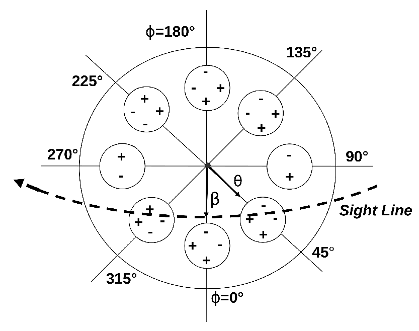
The position of a patch (, ) affects the density gradient along and . For a given patch, different cuts of a line of sight will cause different profiles. Here, we calculate the profiles for typical patch positions in the open field line region, with various impact angles. Figure 12 is the sketch map of the positions of the discussed patches.


 |
| (f) |
 |
| (g) |
Firstly we consider a patch located in the meridional plane with . Sight lines cutting the patch with different give different polarization profiles, as shown in Fig. 13. For , the dominating density gradient is , which is large and has a single sign at all the phases, and is small. The circular polarization keeps to be of the right hand. When increases to be , there exits a little sign reversal of CP in the trailing side of the profile, mainly because is relatively strengthened. For the sight line cuts across the patch center of , reaches its minimum, dominates. The weak circular polarization shows a sign reversal. For large , negative dominates again gradually, which gives the reversal of weak CP and then the left hand CP.
Now, we consider the discrete patches (see Fig. 12) located at different positions around the magnetic axis with , , , , , and . The polarized profiles from cutting through the inner, central and outer parts of the patch are plotted for each patch in Fig.14. Similar to the patch of , the profiles always have a single sign, or the sign reversal, or the opposite sign for the line of sight cutting the inner, central and outer parts of a patch. For the patches at and , we have when the line of sight cuts across the central part of the patch. The profiles for the patch at has almost the same dependence on as the patch of , except for the reversed circular polarization. For other patches away from the meridional plane, the profiles always depend on the variation of and as listed in Table 1. But for patches with not close to or , the density gradient along dominates the sign of circular polarization, because the rotation-induced distortions are weak. For convenience, we mark the final sign of the profile for different in each patch of Fig. 12.

For a given patch, even when the impact angle is fixed, the polarization profiles will be different for various emission heights. The polarized emission from two symmetrical patches with a fixed but different height (10, 20 and 40, respectively) are shown in Fig. 15. Naturally profiles gradually become wider with the increasing of height. They also gradually shift towards an earlier phase due to the aberration effect. The most important is the evolution of the circular polarization with emission heights. At a low height of 10, two components have different signs of CP, and each with one sign only. At a height of 20 (the middle panel), each component has the sign reversal of CP. At a height of 40, each component has one single sign of CP again without reversal but the opposite hand compared to those at 10 . This is mainly because at different heights, the sight lines with a fixed cut through the inner, middle and outer parts of the patches, which should have different circular polarization due to the dominating of .
4 Emission from open field line region

In general, a dipole field is assumed for pulsar magnetosphere. The tangential points of the field lines of can produce emission detectable for a given line of sight . Here is the angle of the sight line from the magnetic axis , and when the sight line goes to the meridional plane. Curvature radii are different for the tangential points at different heights, so that characteristic emission frequencies are different. This is the basic principle for the “radius to frequency mapping”. However, the emission from one height actually has a wide-spread spectrum, the characteristic frequency is only the frequency of the peak-intensity.
In fact, one receives the emission from the whole radiation region as long as the line is of in the open field line region (see Fig. 16). The retardation effect should be considered for the emission from different heights. The emission profile from the whole open field line region is given by
| (20) |
Here , , and are given by equation (16), and is the retarded phase for the emission from different heights.
 |
| (a) a patch with , |
 |
| (b) a patch with , |
 |
 |
| (a) , , | (b) , , |
The emission from a patch in the meridional plane with is plotted in Fig. 17a, with the polarization generated at different phases and heights. The peak intensity (given by equation 16) varies with the heights. The significant contribution to the integrated emission profiles in the bottom panel comes from the region of 8–20. For and , the emission from this patch points away from the observer (see the sketch map of Fig. 16). The dominating contribution comes from the peak height around for the maximum of plasma density (see the dashed line in the left panel of Fig. 17a). For the patch with a higher and wider emission region of (Fig. 17b), the dominating emission comes from the height of about . There the aberration and retardation effects are rather strong, and the phase for the peak intensity and CP are shifted to an early phase.
We plot the emission profiles from the peak height in Fig. 18, which are very similar to the integrated total intensity and polarization profiles. The emission from the peak height always has a sign reversal of the circular polarization, because the density gradient along the magnetic azimuth has the sign reversal. The aberration and retardation effects are very weak for and the depolarization effect is also negligible.
 |
 |
| (a) core model | (b) cone model |
We noticed that the polarization profiles from a patch are almost the same for different frequencies. If the patch is wide and the density gradient is small, e.g. the almost uniform distribution, the net circular polarization from a patch should be very small. Note however that the peak height is different for different frequencies, and the integrated circular polarization may change for different frequencies.
For the core density model, the emission region of does not have an upper limit (see Fig. 16). The intensities from various emission heights, up to thousands of , are still significant compared with that from the peak height of (see Fig. 19a). It is related to the integrand term in equation (16), which determines the final value of . The density variation can be written as
| (21) |
and plotted by the dashed line in Fig. 19a. The total emission profile is very wide in phase because of the retarded emission from large heights, and the polarization will also be vanished.
 |
| (a) core model |
 |
| (b) cone model |
In a practical case, the damping of the Lorentz factor of a particle along is natural. For example, an exponential decay of the Lorentz factor was introduced by Qiao et al. (2001) to analyze the inverse Compton scattering process in the magnetosphere. Here we take the slow variation of the Lorentz factor with height as
| (22) |
where is the energy for the secondary particles near the neutron star polar cap, and is the damping factor, and we calculate the total emission profiles as shown in Fig. 20a. The emission region is constrained to be between and . The total polarized profiles resemble to those from a height of (Fig.10). The circular polarization contributed from each height has the same sign, so the final total circular polarization has only one single sign. The total intensity and polarization profiles are asymmetry due to the retardation effect.
For the cone density model, the density and the peak intensity vary with height as shown in Fig. 19b. The emission can be produced even at a very large height. The dominating emission comes from about 30 to 300 . The profiles become very wide (see Fig.20b) because of the strong retardation effect. With the damping of the Lorentz factor of particles as the core model, the total emission profiles and are shown in Fig. 20b. The cone density only produces one profile component, instead of two. Because the emission from low heights are very strong, and two components from a higher regions are weak and only add the outer wings in both sides of the profile from the lower height. The total circular polarization is very weak also, because of the depolarization of the emission from different heights.
5 Discussions and Conclusions
In this paper, we depict the detailed scenery for curvature radiation in rotating pulsar magnetosphere for the first time. The rotation affects the velocity and acceleration of particles and hence the emission property. Circular path approximation for the particle trajectory is used at the emission point to calculate the radiating electric field (see equation 13). The emission from particles at the tangential points of field lines and the nearby field lines in the emission cone is considered for a given phase and height. The polarization profiles from a given height and the whole open field line region are calculated for three possible density distributions in the form of core, cone and patches. We find the following conclusions:
- 1.
Rotation not only shifts the PA curves along the rotation phase, , but also causes an offset of the curve, , both of which are the first-order functions of the emission height. Its influences on and determination follows the second order functions (Fig. 8).
- 2.
Rotation distorts the patterns for the cone more seriously if it originates from larger height and/or smaller impact angle (Fig. 9). The density gradients across the patterns will result in the net circular polarization.
- 3.
- 4.
The central peaked core will have the circular polarization of only one hand, which is usually significant and always has a single sign (Fig. 20a). The cone emission at a large height is separated into two components with the opposite sign reversals for circular polarization. But at a lower height there is only one component with a single sign of . The total circular polarization is very weak because of the depolarization of the emission from different heights (Fig. 20b).
Our calculations for the curvature radiation from particles distributed in the form of core, cone and patches can be compared with the observed pulsar polarization profiles. The sign reversal of circular polarization are always observed in the central component of the mean profile (Lyne & Manchester, 1988; Rankin, 1983; Gil & Snakowski, 1990). Han et al. (1998) pointed that there also exists sign reversal of circular polarization for the cone components for some pulsars. Such observational facts can be explained if the emission comes from central or non-central patches. The CP with a single sign may come from the core emission.
Here we did not consider the possible propagation effects, i.e., the wave mode coupling effect (Wang et al., 2010) in the magnetosphere. Our calculations can explain some pulsar polarized emission, but it can not match various observation facts. It should be noted that we consider just the curvature emission from particles with a single and assume the simple distributions of particle density. The actual energy and density distributions of particles in the magnetosphere are not clear at present. There exist other emission mechanisms, like ICS (Xu et al., 2000), plasma process (Beskin et al., 1988). Moreover, we treated the coherency in a simple way by assuming the coherent bunch to be a huge point charge. However, the actual coherent manner, bunch size and shape affect the radiation pattern (Benford & Buschauer, 1977). We used the vacuum dipole magnetic field as the basic model for our calculation, but there exists the possible distortion of the dipole magnetic field due to rotation, which has not been taken into account (Dyks & Harding, 2004). The magnetic field structure, such as the globally twisted, self-similar, force-free magnetosphere (Thompson et al., 2002), can also lead to the modification of the radiation pattern. All these will make the actual emission pattern much more complicated than the simple calculations presented in this paper.
Acknowledgments
We thank R. T. Gangadhara and Dinesh Kumar for useful discussions and suggestions. This work has been supported by the National Natural Science Foundation of China (11003023 and 10833003).
References
- Backer (1976) Backer D. C., 1976, ApJ, 209, 895
- Benford & Buschauer (1977) Benford G., Buschauer R., 1977, MNRAS, 179, 189
- Beskin et al. (1988) Beskin V. S., Gurevich A. V., Istomin I. N., 1988, Ap&SS, 146, 205
- Blaskiewicz et al. (1991) Blaskiewicz M., Cordes J. M., Wasserman I., 1991, ApJ, 370, 643
- Buschauer & Benford (1976) Buschauer R., Benford G., 1976, MNRAS, 177, 109
- Dyks & Harding (2004) Dyks J., Harding A. K., 2004, ApJ, 614, 869
- Dyks et al. (2010) Dyks J., Wright G. A. E., Demorest P., 2010, MNRAS, 405, 509
- Gangadhara (2005) Gangadhara R. T., 2005, ApJ, 628, 923
- Gangadhara (2010) Gangadhara R. T., 2010, ApJ, 710, 29
- Gil & Snakowski (1990) Gil J. A., Snakowski J. K., 1990, A&A, 234, 237
- Han et al. (1998) Han J. L., Manchester R. N., Xu R. X., Qiao G. J., 1998, MNRAS, 300, 373
- Hibschman & Arons (2001) Hibschman J. A., Arons J., 2001, ApJ, 546, 382
- Jackson (1975) Jackson J. D., 1975, Classical electrodynamics
- Komesaroff et al. (1970) Komesaroff M. M., Morris D., Cooke D. J., 1970, Aplett, 5, 37
- Kumar & Gangadhara (2012) Kumar D., Gangadhara R. T., 2012, ApJ, 746, 157
- Lyne & Manchester (1988) Lyne A. G., Manchester R. N., 1988, MNRAS, 234, 477
- Ochelkov & Usov (1980) Ochelkov I. P., Usov V. V., 1980, Ap&SS, 69, 439
- Qiao et al. (2001) Qiao G. J., Liu J. F., Zhang B., Han J. L., 2001, A&A, 377, 964
- Rankin (1983) Rankin J. M., 1983, ApJ, 274, 333
- Rankin (1993) Rankin J. M., 1993, ApJ, 405, 285
- Rankin & Ramachandran (2003) Rankin J. M., Ramachandran R., 2003, ApJ, 590, 411
- Ruderman & Sutherland (1975) Ruderman M. A., Sutherland P. G., 1975, ApJ, 196, 51
- Thomas & Gangadhara (2007) Thomas R. M. C., Gangadhara R. T., 2007, A&A, 467, 911
- Thompson et al. (2002) Thompson C., Lyutikov M., Kulkarni S. R., 2002, ApJ, 574, 332
- Wang et al. (2010) Wang C., Lai D., Han J., 2010, MNRAS, 403, 569
- Xu et al. (2000) Xu R. X., Liu J. F., Han J. L., Qiao G. J., 2000, ApJ, 535, 354