Aftershock prediction for high-frequency financial markets’ dynamics
Abstract
The occurrence of aftershocks following a major financial crash manifests the critical dynamical response of financial markets. Aftershocks put additional stress on markets, with conceivable dramatic consequences. Such a phenomenon has been shown to be common to most financial assets, both at high and low frequency. Its present-day description relies on an empirical characterization proposed by Omori at the end of 1800 for seismic earthquakes. We point out the limited predictive power in this phenomenological approach and present a stochastic model, based on the scaling symmetry of financial assets, which is potentially capable to predict aftershocks occurrence, given the main shock magnitude. Comparisons with S&P high-frequency data confirm this predictive potential.
1 Introduction
It is not uncommon for financial indexes or asset prices to experience exceptionally large negative or positive returns which trigger periods of high volatility, the case of abnormal negative returns corresponding to market crashes. An understanding of the dynamical response of the market to a main shock is of great interest because it may help, e.g., in the definition of emergency plans for financial crises, or for risk management.
There is a clear analogy between the behavior of volatility after a main financial shock and that of the seismic activity after an earthquake of exceptional magnitude in geophysics [12]. Omori [10], with a subsequent modification by Utsu [16], established an important empirical law describing the frequency of occurrence of seismic events above a given threshold after a main earthquake. The characterizing feature of this law is the decay as a power of time, , of the rate of occurrence of aftershocks above the threshold, indicating the absence of a characteristic time scale in the manifestly non-stationary Omori regime. More precisely, according to Omori the number, , of aftershocks per unit time above a given threshold is given by
| (1) |
where depend on the aftershock threshold , and also on the specific magnitude of the main shock earthquake. Equivalently, the Omori law can be expressed in an integral form as
| (2) |
if , or if , where is the cumulative number of aftershocks up to time after the main shock. Lillo and Mantegna [7] were the first to verify the validity of an analog of the Omori law for the volatility in Finance after a main crash. They also showed [8] that standard dynamical models of index evolution, like GARCH, are not adequate to reproduce financial Omori-like regimes. Several studies [7, 8, 13, 14, 18, 9, 11] verified the presence of Omori regimes under various market conditions, triggered by financial crashes [7, 8, 13, 14, 18], by volatility shocks [9], and even by U.S. Federal Open Market Committee meetings [11]. In particular, the Omori law in finance has been upgraded to a more general characterization of market dynamics by Weber et al. [18], who pointed out that this law holds on a wide range of time scales, with aftercrashes of a main shock playing the role of main crashes for even smaller aftercrashes, etc.
The above mentioned studies make clear the connection between financial Omori processes and long-range dependence of the volatility. They also show that a modulating, time dependent scale for the returns must be considered in order to account for the manifest non-stationarity of the Omori process. At the same time, they emphasize the limits in the predictive value of the Omori law. For example, the parameters and need to be adjusted for each aftershock threshold considered (See below). This holds also for the exponent of the power law decay, which should be expected to be the most robust parameter. In addition, there is no idea of how the parameters could be linked to the magnitude of the main shock. These limits reflect a lack of adequate modeling for the dynamics of financial indexes, especially in regimes like those covered by the Omori law. In recent contributions [3, 4], some of the present authors have proposed a model for the dynamics at high frequency of exchange rates or stock market indexes, which takes into account most of the relevant stylized facts. Among them, the martingale character of index evolution, the manifest non-stationarity of volatility detected in well defined daily windows of trading activity, the anomalous scaling properties of the aggregate return probability density function (PDF) in the same windows, and the strong time autocorrelation of the elementary absolute return. This model for high-frequency data, which applies more general ideas about the time evolution of financial indexes [2, 15, 6], has also been tested [3] by comparing its predictions with the statistics of ensembles of daily histories all supposed to reproduce the same underlying stochastic process. It has been also shown [4] that some arbitrage opportunities revealed by the model could be successfully exploited by appropriate trading strategies.
In the present contribution we address the problem of describing with such a model the Omori processes which may be detected within these daily windows. Our goal is to show that, after proper calibration, this model allows the prediction of the aftershock rate within an Omori regime, given the value of the main shock magnitude. Indeed, we provide analytical expressions for the rate of financial aftershocks with explicit dependence on the magnitude of the main shock and on the aftershocks threshold. By comparing our predictions with high frequency data from the S&P 500 index we show that these quantities are sufficient to determine the Omori response without further fitting parameters. Our success is partly due to the fact that we are able to identify the Omori processes within a context for which non-stationarity is well established [5] and amenable to modeling [3, 4]. In an interday context, the question of the applicability of the models of Ref. [2] to Omori regimes has already been raised in Ref. [6].
This note is organized as follows. In the next Section we briefly recall the model of Refs. [3, 4] and present the procedure of calibration. In the third Section we discuss the selection of Omori-like processes from our database and show how our model can be used to analytically describe these processes. In the fourth Section we compare the results of the properly calibrated model with the statistical records at our disposal for the S&P 500 index. The last Section is devoted to general discussion and conclusions.
2 Model calibration
Let us consider the successive (log-)returns over ten minutes intervals of the S&P 500 index for daily windows from 9.40 a.m., Chicago time, to 1.00 p.m.:
| (3) |
where the time is measured in ten-minute units and we have set at 9.40 a.m.11 1 In order to keep contact with ordinary notations for the Omori law, in this paper we change slightly our usual conventions by shifting the origin of time by one unit with respect to, e.g., Refs. [3, 4]. . A statistics made over the ensemble of 6283 available daily histories from 1985 to 2010 shows [4] that a stochastic process supposed to generate the successive returns in a generic history of the ensemble is consistent with the following joint PDF:
| (4) |
where
| (5) |
with , , and with
| (6) |
This joint PDF is a convex combination of products of Gaussian PDF’s for each individual return. The PDF weights this combination and introduces a nontrivial dependence of the returns from the preceding ones. For , the coefficients make the process increments non-stationary, and modulated by the exponent .

The calibration of the model can be done by direct comparison of its predictions with the main features of the PDF’s of the 10-minute returns ’s, or, alternatively, with those of the aggregate returns [3, 4]. Here we follow the second option. Since the model predicts for the PDF of the aggregate return satisfaction of an anomalous scaling of the form
| (7) |
where the scaling function is expressed as
| (8) |
one can determine through a fitting of the power law -dependence of the moments of . Indeed, for , according to Eq. (7)
| (9) |
with , and provided that the moment exists. In Fig. 1 we report the empirical values for , using Eq. (9) as an ansatz. To calibrate , we make a linear data regression for , since for higher moments a multiscaling behavior [17] is detected (See Fig. 1). The result is .
A particularly simple expression for the joint PDF is achieved if the integration on can be worked out explicitly in Eq. (4). This is indeed the case if we choose an inverse-gamma distribution for [6]. Equivalently, we may set
| (10) |
where the exponent determines the long-range behavior of according to for , and is a scale parameter determining the distribution width. Performing the integration on in Eq. (4) we obtain a multi-variate Student PDF:
| (11) |
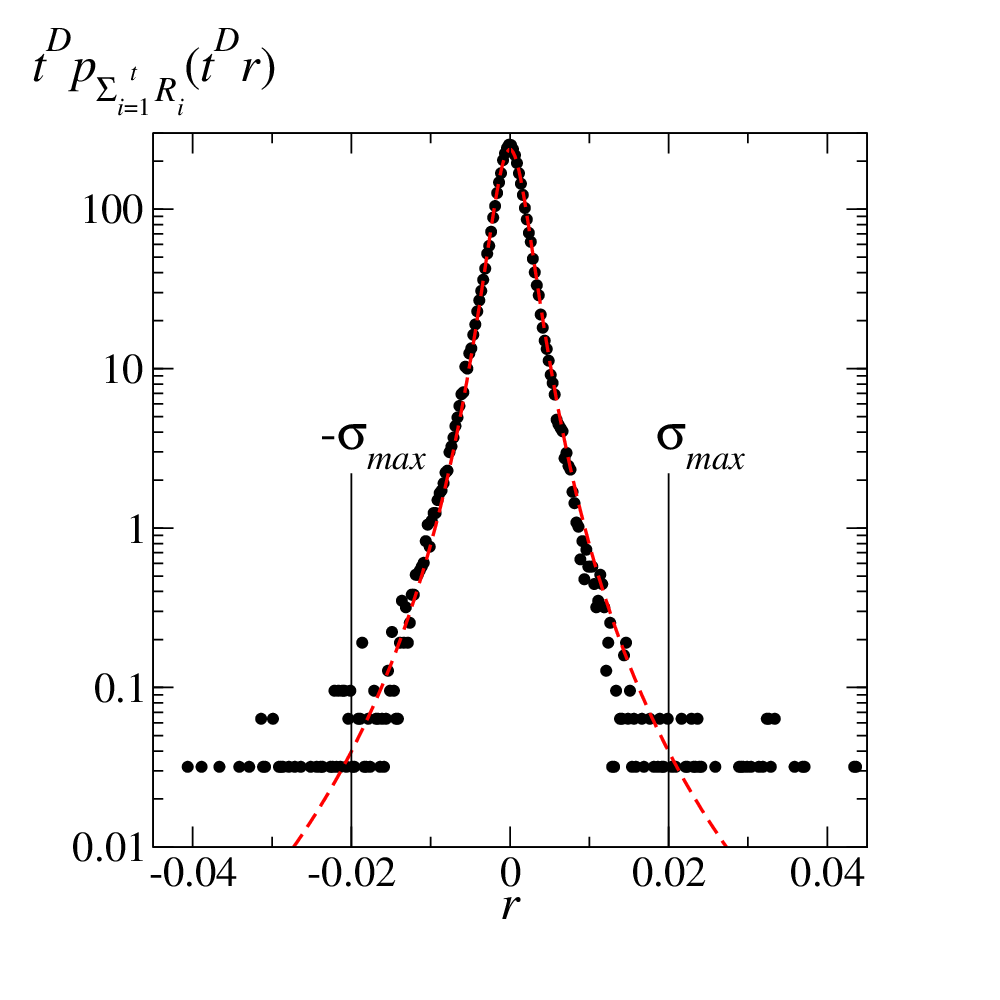
As we will show in the following, an explicit form for enables us to obtain a simple analytic expression for . Unlike in previous papers [3, 4], we thus choose here the functional form in Eq. (10) for . Besides , the other parameters of the model, and , are calibrated by first data-collapsing the empirical PDF’s for according to Eq. (7) with , and then by fitting and on this data-collapse using Eq. (11) with . The result is given in Fig. 2. In summary, the result of the calibration procedure is the triple .
The ensemble of histories at our disposal is relatively poor. This implies, as can be appreciated in Fig. 2, that some rare events fall significantly out of the scaling function, since a much larger number of histories would be needed to correctly characterize their frequency of occurrence. The multiscaling behavior shown in Fig. 1 could be at least partly related to this effect. The Omori events are precisely related to extreme events. In order to obtain a reliable statistics of the aftershocks, we impose thus an upper bound to the absolute value of the returns ’s included in our empirical analysis (See Fig. 2). Once done this, the overall agreement of the empirical data with the various model predictions gives a convincing validation of the model itself (See also [4]). Still, the agreement shown in what follows with respect to the Omori processes must be intended as a first important result, which calls for more extensive analysis also in terms of the calibration procedure.
3 Aftershock prediction
As already mentioned above, in the present analysis we are going to identify and select Omori processes, which are manifestations of non-stationarity, within a process which manifestly turns out to be with non-stationary returns in its ensemble of daily realizations. This is a simplification which marks an important difference with respect to the problem of modeling the Omori regimes revealed in Refs. [7, 8, 13, 14, 18, 9, 11], where they were extracted from single time series expected to be globally stationary on long time scales. In the perspective of our approach here, dealing with a process which is by itself time-inhomogeneous offers the advantage that the selection of Omori processes does not imply the need of identifying how their non-stationarity emerges from an otherwise stationary global behavior. In a version of our model suited for describing single, long time series of returns [15, 19], the necessity to consider random exogenous factors influencing the market, leads us to switch-on at random times some time-inhomogeneities formally similar to those characterizing the model of the previous Section. This is achieved by setting concomitantly with these random events (See also [2, 3, 6, 1]). In such a context it is not a priori clear whether or not the start of an Omori process should imply putting in correspondence with the time of the main shock. This difficulty is also accompanied by the need of implementation of a more complicated calibration procedure [19] with respect to the one presented here.
As shown below, remarkable results of our analysis in this note are:
- 1.
that the selected processes are legitimately classified as Omori-like in the sense that they can all be fitted by the Omori law;
- 2.
that the description one obtains for them based on the model presented in the previous Section contains explicit dependencies on the intensities of the main shock and on the aftershocks thresholds.
This endows our approach to the Omori regimes of a predictive potential which, if confirmed by further analysis, could be exploited by decision-makers under crisis conditions.
We select as Omori processes all those histories in the above S&P 500 ensemble for which the initial absolute return, , besides being smaller than , also exceeds a main shock threshold . At variance with the analysis in Refs. [7, 8, 13, 14, 18, 9, 11], we consider, in place of a single time series, groups of histories for which . As far as the aftershocks are concerned, we record for each of these histories the elementary returns which exceed in absolute value an aftershock threshold and are below the main shock value : , for . The parameter is an important one to be fixed in any analysis of the Omori law. Again, by imposing the aftershock magnitude to be smaller than that of the main shock we reduce the influence of extreme events in our limited dataset. We decided to search for main shocks occurring right at the beginning of the daily time window described by our model for two main reasons. In first place the ensemble average volatility on 10 minutes intervals is maximal in the first interval. Secondly, a main shock occurring right at the beginning of the time window leaves the maximum possible time for the development of the subsequent Omori process. While we will limit ourselves below to discuss such optimal case, different choices are of course possible.
According to the above selection procedure of the Omori processes, the cumulative number of aftershocks after a main shock of magnitude is given by
| (12) |
where is the indicator function, yielding if and zero otherwise. Using Eq. (11), through a change of variable it is straightforward to show
| (13) | |||||
If in the considered ensemble of histories there are realizations in which we register a main shock, i.e., , then the cumulative number of aftershocks is obtained through the sample average
| (14) |
where we stress the fact that each is conditioned to the main shock magnitude . Notice that since with the available dataset the selected main shocks constitute a small sample (see next Section), we use here the sample average rather than the ensemble one to get the number of aftershocks conditioned to .

| \svhline | |||
|---|---|---|---|
4 Comparison of the model predictions with the statistics of aftershocks
Our choice for the thresholds and is such that the absolute first returns for which are quite exceptional. They occur with frequency in our ensemble; Only 3 realizations have and are thus excluded. Accordingly, we analyze the averaged of aftershocks for these main shocks. A first point to clarify is whether the recorded rates are well fitted by the Omori law in Eq. (2). This is shown in Fig. 3, where many sets of data for , obtained with different aftershocks thresholds , are indeed fitted by the Omori Eq. (2). In Table 1 one also realizes that , and need to be varied for each in order to reach a satisfactory fit. In particular, by changing and it is even possible to obtain reasonable fittings also with (See also [9]). This parameters variability makes it very difficult to use the Omori law to predict the aftershock occurrence for a given main shock magnitude and aftershock threshold.

Model predictions on the same set of data fitted in Fig 3 are instead given in Fig. 4. Dashed lines in Fig. 4 are obtained on the basis of Eqs. (13,14) with the parameters resulting from the calibration discussed in Section 2. The only difference among the curves is the value of the aftershock threshold . The agreement of the analytical predictions with the data and the sensitivity of the curves to the variation of the aftershock threshold are remarkable. This shows that our model potentially provides a satisfactory and parameter-free description of Omori processes.
5 Conclusions
We have shown here in the case of the S&P 500 index, that a model suited for the description of the high frequency market dynamics allows also to predict Omori regimes following exceptional extreme events. Within the class of events considered, the model specifies the dependence on the main shocks intensities and on the aftershocks threshold. As such, its description goes far beyond the limits of the Omori phenomenological law.
Besides providing a further validation of the model of Refs. [3, 4], the results presented here encourage to extend similar analysis to cases in which the Omori processes are to be selected within a process which is globally stationary. For the modeling of these processes, our recipe [19] is that of switching-on at random some non-stationarities ascribable to coefficients like the defined above. Global stationarity of the process on long time scales is then guaranteed by the fact that empirical averages are in this case made by considering time intervals sliding along the single long history [19]. While it is conceivable that in many cases main shocks are localized close to resets of the time inhomogeneity, this is not true in general. Some attempts to strictly identify main shocks with restarts of them inhomogeneity in the model () already gave some preliminary agreement with the data. A more general discussion is however needed [19].
Acknowledgements.
This work is supported by “Fondazione Cassa di Risparmio di Padova e Rovigo” within the 2008-2009 “Progetti di Eccellenza” program.References
- (1) A. Andreoli, F. Caravenna, P. Dai Pra, G. Posta, Scaling and multiscaling in financial indexes: a simple model, Adv. Appl. Prob. (in press, 2012) [arXiv:1006.0155].
- (2) F. Baldovin and A.L. Stella, PNAS 104, 19741 (2007).
- (3) Baldovin, F., Bovina, D., Camana, F. and Stella, A.L.: Modeling the Non-Markovian, Non-stationary Scaling Dynamics of Financial Markets. In F. Abergel, B. K. Chakrabarti, A. Chakraborti and M. Mitra (eds.) Econophysics of order-driven markets (1st edn), pp. 239–252, New Economic Windows, Springer (2011).
- (4) F.Baldovin, F.Camana, M. Caporin and A. L. Stella, Ensemble properties of high frequency data and intraday trading rules, submitted (2012) [arXiv:1202.2447].
- (5) K.E. Bassler, J.L. McCauley, and G.H. Gunaratne, PNAS, 104, 17287 (2007).
- (6) D. Challet and P.P. Peirano, The Ups and Downs of Modeling Financial Time Series with Wiener Process Mixtures, submitted (2012) [arXiv:0807.4163].
- (7) F. Lillo and R. N. Mantegna, Phys. Rev. E 68, 016119 (2003).
- (8) F. Lillo and R. N. Mantegna, Physica A 338, 125 (2004).
- (9) G.-H. Mu, W.-X. Zhou, Physica A 387, 5211 (2008).
- (10) F. Omori, J. Coll. Sci. Imp. Univ. Tokyo 7, 111 (1984).
- (11) A.M. Petersen, F. Wang, S. Havlin, and H. Eugene Stanley, Phys. Rev. E 81, 066121 (2010); Phys. Rev. E 82, 036114 (2010).
- (12) Scholz, C. H. The Mechanics of Earthquakes and Faulting, Cambridge University Press, New York (2002).
- (13) F. Selçuk, Physica A 333, 306 (2004).
- (14) F. Selc-uk, R. Genc-ay, Physica A 367, 375 (2006).
- (15) A.L. Stella and F. Baldovin, J. Stat. Mech. P02018 (2010).
- (16) T. Utsu, Geophys. Mag. 30, 521 (1961).
- (17) F. Wang, K. Yamasaki, S. Havlin, H.E. Stanley, Phys. Rev. E 77, 016109 (2008).
- (18) P. Weber, F. Wang, I. Vodenska-Chitkushev, S. Havlin, and H. E. Stanley, Phys. Rev. E 76, 016109 (2007).
- (19) F. Baldovin, A.L. Stella and M. Zamparo in preparation.