Local electric current correlation function in
an exponentially decaying magnetic field
Abstract
The effect of an exponentially decaying magnetic field on the dynamics of Dirac fermions in dimensions is explored. The spatially decaying magnetic field is assumed to be aligned in the third direction, and is defined by , with . Here, is a dimensionless damping factor and is the magnetic length. As it turns out, the energy spectrum of fermions in this inhomogeneous magnetic field can be analytically determined using the Ritus method. Assuming the magnetic field to be strong, the chiral condensate and the local electric current correlation function are computed in the lowest Landau level (LLL) approximation and the results are compared with those arising from a strong homogeneous magnetic field. Although the constant magnetic field can be reproduced by taking the limit of and/or from , these limits turn out to be singular, especially once the quantum corrections are taken into account.
pacs
11.15.-q, 11.30.Qc, 11.30.Rd, 12.20.-m, 12.20.DsI Introduction
The effects of magnetic fields on systems containing relativistic fermions are subject of intense theoretical studies over the past two decades. These effects include a wide range, from condensed matter physics [1] to high energy physics [2] and cosmology [3]. Theoretical studies deal in the most of these works with the idealized limit of constant and homogeneous magnetic fields. However, this limit is only reliable as long as the scale of field variation is much larger than the Compton wavelength of the fermionic system. As it is shown in [4], strong and homogeneous magnetic fields lead to the formation of fermion bound states even in the weakest attractive interaction between the fermions. This phenomenon, known as magnetic catalysis of dynamical chiral symmetry breaking [5], is essentially based on a dimensional reduction from to dimensions in the presence of strong homogeneous magnetic fields in the regime of LLL dominance. However, as it is demonstrated recently in [6], massless Dirac electrons can also be confined by inhomogeneous magnetic fields in graphene, which is a single layer of carbon atoms in a honeycomb lattice. Electrons in graphene are described by a massless two-dimensional, time-independent relativistic Dirac equation. As it is shown in [6], magnetic quantum dots can be formed, if one neglects the effects of electron spin and solves the Dirac equation in the presence of a square well magnetic barrier of width , , directed perpendicular to the graphene plane, with , and the Heaviside step function. A circularly symmetric magnetic quantum dot arises then by a radially inhomogeneous magnetic field (see [6, 7] for more details). In [8], the bound state solutions and the spectra of graphene excitations in the presence of an inverse radial magnetic field, with , is studied. Analytical solutions for the Dirac equation in the presence of double or multiple magnetic barriers are presented in [9]. The bound spectra of electrons in a magnetic barrier with hyperbolic profile is studied in [10].
In the present paper, we will focus, in particular, on the solution of Dirac equation in the presence of an exponentially decaying magnetic field. Analytical solution of a quasi-two-dimensional Dirac equation including the spin of a single electron in a magnetic field of constant direction with arbitrarily strong exponentially depending variation perpendicular to the field direction is firstly presented in [11]. In [12], the probability density and current distributions of Dirac electrons in graphene in the presence of an exponentially decaying magnetic field are determined. The formation of chiral condensate induced by exponentially decaying magnetic fields, in dimensions, is studied in [13]. The vacuum polarization tensor of dimensional scalar Quantum Electrodynamics in the presence of an inhomogeneous background magnetic field, arising from a general plane wave basis for the underlying gauge field, is computed recently in [14]. In order to demonstrate the nonlocal features of quantum field theory in the presence of inhomogeneous background magnetic fields, the vacuum polarization tensor is defined to be local. This turns out to be a useful task providing local information about the nonlocal nature of fluctuation-induced processes [14]. In the present paper, following the same idea as in [14], we will define a local electric current correlation function (local electric susceptibility), and compute it in the presence of a strong and exponentially decaying magnetic field in the LLL approximation. Eventually, we will compare the result with the electric current correlation function arising from a strong homogeneous magnetic field and discuss the effects of inhomogeneity of the background magnetic field.
The organization of the paper is as follows: In Sec. II.1, we will briefly review the Ritus eigenfunction method [15] by solving the Dirac equation in the presence of a constant and homogeneous magnetic field. In Sec. II.2, we will introduce an exponentially decaying magnetic field , which is assumed to be aligned in the third direction, with given by . Here, is a dimensionless damping parameter and is the magnetic length. Using the Ritus method, the energy eigenvalues and eigenfunctions of a dimensional Dirac equation in the presence of will be determined. In Sec. III, we will determine the chiral condensate , using the fermion propagator in the presence of strong homogeneous (Sec. III.1) and exponentially decaying magnetic fields (Sec. III.2) in the LLL approximation. We will show that whereas in a strong homogeneous magnetic field is constant, in an exponentially decaying magnetic field depends nontrivially on a dimensionless variable , defined by . In Sec. IV, the local electric current correlation function (local electric susceptibility) will be computed in the presence of strong homogeneous (Sec. IV.1) and exponentially decaying magnetic fields (Sec. IV.2) in the LLL approximation. Here, denotes the three spatial directions. As it turns out, in the regime of LLL dominance the electric susceptibility in the perpendicular direction relative to the external magnetic field (i.e. for ) vanishes in both homogeneous and inhomogeneous magnetic fields. The longitudinal component of , denoted by , turns out to be constant in a homogeneous magnetic field and depend nontrivially on the dimensionless variable in an exponentially decaying magnetic field. In Sec. V, we will compare the results for the chiral condensate and the local electric current correlation function arising from homogeneous and inhomogeneous magnetic fields and show that the limits as well as are singular. In other words, although in the limits and/or , we get , but the values of and arising from an exponentially decaying magnetic field in these limits are not the same as and arising from a homogeneous magnetic field. This demonstrates the nonlocal features of the quantum vacuum in a strong and spatially decaying magnetic field. As is indicated in Sec. VI, which is devoted to our concluding remarks, the results of this paper are relevant for high energy physics as well as condensed matter physics.
II Electrons in external magnetic fields
Ritus eigenfunction method [15] is a powerful tool to study the dynamics of electrons in external electromagnetic fields. It is recently used in [16] to solve the Dirac equation in the presence of a uniform magnetic field in 2+1 dimensions, a uniform electric field in 1+1 dimensions and an exponentially decaying magnetic field in dimensions (see also [13]). In [17, 18], the Ritus method is used to solve the dimensional Dirac equation for massless fermions in the presence of a constant magnetic field. In Sec. II.1, we will briefly review the results from [18] and will present the solution of the Dirac equation for a single massive electron in the presence of a constant magnetic field in dimensions. This will fix our notations. In Sec. II.2, we will use the same method and will solve the Dirac equation for a massive electron in an exponentially decaying magnetic field. Our results coincide with the result presented in [13], although our notations are slightly different. We will also present the final form of the fermion propagator in the presence of a uniform and an exponentially decaying magnetic field in Secs. II.1 and II.2, respectively. The results presented in this section will then be used in Sec. III to determine the chiral condensate, and in Sec. IV the local electric current correlation function in the presence of uniform and non-uniform magnetic fields.
II.1 Electrons in constant magnetic fields
Let us start with the Dirac equation of a single electron in dimensional Minkowski space in a background electromagnetic field
| (II.1) |
where and is the electromagnetic potential. Here, and are the electron’s mass and electric charge, respectively. The aim is to solve (II.1) and to eventually determine the fermion propagator in the presence of background constant magnetic field , aligned in the third direction. Such a constant magnetic field, is built, for instance, by choosing the gauge field in the Landau gauge as . To solve (II.1), we use, as in [17, 16], the Ansatz . Here, is a diagonal matrix satisfying
| (II.2) |
and is a free spinor, that describes an electron with momentum and satisfies . The Ritus eigenfunction and the Ritus momentum in (II.2) are unknown and shall be determined in what follows. The matrix is determined by solving the eigenvalue equation
| (II.3) |
that arises directly from (II.2). Using , with and the field strength tensor , with non-vanishing elements , and choosing, without loss of generality, the Dirac -matrices as , and , where are the Pauli matrices, (II.3) reads
| (II.4) |
Here, with a identity matrix. To solve (II.4), we use the fact that in the Landau gauge, the operator commutes with , and , and therefore has simultaneous eigenfunctions with these operators. The eigenvalues of these operators, defined by the eigenvalue equations
| (II.5) |
label the solutions of Dirac equation (II.1) in the background magnetic field. Using (II.3), the definition of and (II.5), it can be shown that the four-momentum satisfies , and is therefore given by
| (II.6) |
Before solving (II.6), let us determine the components of Ritus momentum , which turns out to play an important role in this method. To do this, we consider (II.2), and use the Ansatz
| (II.7) |
with the projectors [17]
| (II.8) |
Plugging first from (II.7) in the left hand side (l.h.s) of (II.2), and then comparing the resulting expression with the expression arising from the right hand side (r.h.s.) of (II.2), where again from (II.7) and the Ansatz is used,11 1 The form suggests that . Moreover, we have fixed , where according to (II.5) are the eigenvalue of , respectively. we arrive at (II.6), with given by . This will fix .22 2 Note that the general solution for is either or . Here, we have chosen to have the same notation as in [18].
Let us now turn back to the solution of (II.6), whose form suggests a plane wave Ansatz in the and directions,
| (II.9) |
where and . Plugging (II.9) in (II.7), and using for the projectors defined in (II.8), the general solution for is given by
| (II.10) |
where
| (II.11) | |||||
To determine , it is enough to replace from (II.10) in (II.6) to arrive at
| (II.12) |
Renaming the discrete quantum numbers in the four-momentum by , and choosing a new coordinate , with the magnetic length defined by , the differential equation in (II.12) can be reformulated in the form of the differential equation of harmonic oscillator, whose center lies in and oscillates with the cyclotron frequency [16],
| (II.13) |
As it turns out, the solution to the above equation can be given in terms of parabolic cylinder function [17, 16]
| with | (II.14) |
where is, in general, given by
| (II.15) |
Here, labels the energy (Landau) levels. In the rest of this paper, we will work with . According to (II.15), for sgn, the condition that for , fixes the spin orientation of the electrons in the LLL to be positive (). In this case will be given by for all values of [17]. For this specific choice, the final result for is the same as the result presented in [18],
Hence, for , only the positive spin solution contributes in the LLL, characterized by . In other words, is undefined and is to be neglected, whenever it appears in a computation.
The energy dispersion relation for an electron in the presence of a constant magnetic field is determined by the Ritus momentum
| (II.17) |
and is given by
| (II.18) |
The Ritus eigenfunction from (II.10) can be used to determine the fermion propagator in the presence of a uniform magnetic field. To do this, the Ansatz for the electron is to be generalized to a system including particles and antiparticles. Defining the associated creation and annihilation operators, and following the standard steps to determine the propagator [19], the fermion propagator in the presence of a constant magnetic field is given by (see also [18])
where , is given in (II.11) with from (II.1), and the Ritus momentum is given in (II.18). The same expression appears also in [18]. Since we are working with , and the spin orientation of the electrons are already fixed in the LLL to be positive, no spin projector appears in (II.1), as in the fermion propagators presented in [17]. To understand this, let us notice again that the facts that LLL includes only the positive spin solution, and that negative spin solutions contribute only to the higher Landau levels, are explicitly implemented in the choice for positive spin solution , and for negative spin solution in (II.1). In Sec. II.2, we will use the above method to determine the energy dispersion relation and the propagator for electrons in the presence of exponentially decaying magnetic fields.
II.2 Electrons in exponentially decaying magnetic fields
In this section, the Ritus eigenfunction method will be used to determine the energy levels of a single fermion in the presence of an exponentially decaying magnetic field , aligned in the third direction. Here, is the magnetic field at , is a dimensionful damping parameter. Later, we will set , where is a given dimensionless damping parameter and . The dynamics of this electron in such an inhomogeneous magnetic field is described by the Dirac equation (II.1). To solve it, we fix the gauge, in contrast to the previous case, by , as in [13]. With this choice of , the case of constant magnetic field will be recovered by taking the limit (or equivalently ) in the classical level. Using the Ansatz , with satisfying (II.2), and following the same steps leading from (II.2) to (II.6), we arrive at
| (II.20) |
where are the eigenvalues of third Pauli matrix, . Using in analogy to (II.7), a plane wave Ansatz for ,33 3 Note that the plane wave Ansatz is justified by , where is defined by , as in Sec. II.1.
| (II.21) |
with defined in (II.8), and , we arrive first at
| (II.22) | |||||
In the above equations, where is a dimensionless variable defined by . Moreover, , and are given as in the previous section [see below (II.9)]. Comparing (II.22) with the differential equation
| (II.23) | |||||
satisfied by
| (II.24) |
where is the associated Laguerre polynomial, the quantum numbers and are given by
| (II.25) |
Note that the indices and in are to be positive integers. This implies the following quantization for and
| (II.26) |
leading to , with , and
| (II.27) |
In (II.26), is the greatest integer less than or equal to . As it is shown in [11, 12, 13], is associated with certain constant length , through the relation
| (II.28) |
where is a fixed length. At this stage, let us compare, from (II.27) with appearing in (II.15) for .44 4 Comparing to (II.15), from (II.27), is in general given by . As it turns out, in the case of exponentially decaying magnetic field, labels the energy levels. In analogy to the case of constant magnetic field, to keep from (II.27) positive, the electron spin orientation in the lowest energy level, characterized by , is fixed to be positive (). In this case, we have . What concerns the quantum numbers and , for , we get , that guarantees . In analogy to the solutions (II.1), for the constant magnetic fields, we arrive therefore at
| (II.29) |
with for positive spin solutions and
| (II.30) |
with , for negative spin solutions. Using the orthonormality relations of associated Legendre polynomials , the normalization factor is given by
Using finally the projection matrices , the solution for can be brought in the form similar to the Ritus eigenfunction (II.10) and (II.11) for constant magnetic field,
| (II.31) |
with
Using the orthonormality conditions for the associated Laguerre polynomials, , presented in App. A, it is straightforward to derive the closure and the orthonormality relations for ,
| (II.33) |
as well as
| (II.34) |
In the above relations, , , and , , and
| (II.35) | |||||
with given in (II.8). These relations are similar to the results presented in [13]. Note that the term proportional to isolates the contribution of the lowest energy level, characterized by . This term is also proportional to , implying that the spin orientation in the lowest energy level for is positive. What concerns the contribution of higher energy levels, we had to distinguish between , and cases. This is because plugging from (II.31) and (II.2) in the l.h.s. of (II.34), leads in general to the orthonormality relations similar to (A.1) in App. A, where and are not necessarily equal. In App. A, the orthonormality relation (A.1) is determined separately for , and . Using these results, it is straightforward to derive the remaining terms in (II.35), arising from higher energy levels.
To determine the Ritus momentum , we insert the above solution (II.31) and (II.2) for in (II.2). After some straightforward algebraic manipulations, where we use the recursion relations of the Laguerre polynomials , we arrive at
| (II.36) |
Here, and . Comparing the r.h.s. of (II.36) with (II.2), we get , which can alternatively be given in terms of and as
| (II.37) |
with . Using (II.37), the energy dispersion relation of a single electron in an exponentially decaying magnetic field is given by
| (II.38) |
which is to be compared with the energy dispersion relation of an electron in the presence of a constant magnetic field from (II.18). Let us notice, that although labels the energy levels, in contrast to the case of constant magnetic field, determines the ordering of energy levels. Because of the above mentioned conditions for the integer quantum numbers , (or ), some value of are not allowed. The simplest way to determine , is to write it in terms of and as . Choosing , then turns out to be for (or all values of ), for , for , etc. In Secs. III and IV, the summation over energy levels in an exponentially decaying magnetic field will be replaced by . Here, is a generic function, that depends on the quantum numbers and . According to the above descriptions, the lowest energy level is then characterized by , or equivalently by .
Following the description presented at the end of the previous section, the fermion propagator of an electron in an exponentially decaying magnetic field is given by (see also [13])
where and are given in (II.31)-(II.2) and (II.37), respectively. Using (II.2) and the closure of from (II.33), it is easy to verify
| (II.40) |
where . Here, as in the case of constant magnetic fields, since we are working with , the spin orientation in the lowest energy level is fixed to be positive, and the negative spin electrons contribute only to higher energy levels. These facts are explicitly implemented in the choice for positive spin solution and for negative spin solution in (II.29) and (II.30), respectively.55 5 In other words, is undefined and is to be neglected, whenever it appears in a computation.
III Fermion condensate in external magnetic fields
In this section, we will determine the fermion condensate in the presence of constant and exponentially decaying magnetic fields. The fermion condensate is defined by [20]
| (III.1) |
where is the fermion propagator in the presence of an external magnetic field, in general. In [5], Schwinger’s proper-time formalism is used to determine in a constant magnetic field in the LLL approximation. In this section, we will use the Ritus method, and in particular, our results from the previous section to determine first in a constant and then in an exponentially decaying magnetic field, in the LLL approximation, at finite temperature and chemical potential.
III.1 in constant magnetic fields
To determine the fermion condensate in a constant magnetic field, let us replace from (II.1) in (III.1). Performing the traces over -matrices, we arrive at
| (III.2) | |||||
where according to (II.17), the for is defined by . In the LLL approximation, we shall set . Using the definition of from (II.1), and after performing the integration over ,
| (III.3) |
we arrive at
| (III.4) |
where . The dimensional reduction into two longitudinal dimensions , which occurs whenever the LLL approximation is used [5], can be observed in (III.4). To evaluate (III.4), we use
| (III.5) |
which yields the fermion condensate in the presence of a constant magnetic field in the lowest Landau level,
| (III.6) |
Here, is an appropriate momentum cutoff. This result coincides exactly with the result presented in [5], where the method of proper-time is used. Note that although no integration over the coordinates is performed here, the condensate (III.6) is constant in . This is mainly because of the special form of from (II.1) and arises from the integration over in (III.3). In Sec. III.2, we will show that in the presence of an exponentially decaying magnetic field, the condensate in the LLL depends nontrivially on . Let us also notice that in massless QED, the mechanism of magnetic catalysis [4, 5] is made responsible for dynamically breaking of chiral symmetry and the generation of a finite dynamical mass in the LLL. Moreover, as it is shown in [21], apart from a dynamical mass induced by the external magnetic field in the LLL, an anomalous magnetic moment is also induced, so that the dynamical mass in the LLL is to be replaced by the rest energy , which is a combination of the induced dynamical mass and the anomalous magnetic moment in the LLL. In this paper, we do not consider the effects of dynamically induced anomalous magnetic moment on the dynamically generated fermion mass. The latter arises either as a solution of an appropriate Schwinger-Dyson equation in a ladder approximation or by solving a corresponding gap equation to an appropriate effective potential in the mean field approximation. In what follows, we will compute from (III.6) at finite temperature and finite density . To do this we use the standard imaginary time formalism, and replace in (III.4) by , where is the Matsubara frequency labeled by . Thus the integration over is to be replaced by
| (III.7) |
where . The fermion condensate at finite and is therefore given by
To evaluate the integration over and the summation over , the relation
| (III.9) | |||||
from [22] will be used. This relation (III.9) is originally derived in [23] for . In (III.9), is the Hurwitz zeta function defined by , where any term with is excluded. In an evaluation up to , we get finally
| (III.10) | |||||
where is the Euler-Mascheroni number and the polygamma function, defined by . It arises by an appropriate regularization of using
| (III.11) |
In (III.10), the divergent term is neglected, and the identity is used.
III.2 in exponentially decaying magnetic fields
The chiral condensate in an exponentially decaying magnetic field is given by (III.1), where is to be replaced by from (II.2). Performing the trace of Dirac matrices, we get first
| (III.12) | |||||
where, according to (II.37), and . The expression on the r.h.s. of (III.12) includes the contributions of all energy levels, denoted by and , and the terms proportional to and correspond to the contributions of electrons with positive and negative spins, respectively. In the presence of strong magnetic fields, assuming that the dynamics of the system is solely determined by the LLL, the fermion condensate is given by
| (III.13) | |||||
in contrast to (III.4). The -dependent factor behind the integral arises by setting in (III.12) and using and
Note that in (III.13), the same dimensional reduction to two dimensions, as in the case of constant magnetic field, occurs. Evaluating the -integration using (III.5), we get
| (III.14) | |||||
In contrast to (III.6), the fermion condensate in an exponentially decaying magnetic field, (III.14), depends on with , and , the magnetic length corresponding to , the value of the magnetic field at . Following the same method to introduce finite temperature and chemical potential as in the Sec. III.1, we arrive at
| (III.15) | |||||
In Sec. V, we will compare the chiral condensates (III.6) and (III.14), as well as (III.10) and (III.15), arising from constant and exponentially decaying magnetic fields, respectively.
IV Local electric current correlation function in external magnetic fields
In this section, we will determine the local electric current correlation function in homogeneous and inhomogeneous magnetic fields. It is defined generically by
| (IV.1) |
with
| (IV.2) | |||||
where are the spatial dimensions, and the sub- and superscripts on and indicate the contribution of each energy (Landau) level to the local electric current correlation function and the fermion propagator , respectively. Moreover, and . Up to an integration over ,66 6 The direction is specified, because of the specific Landau gauge, which fixes as is described in Sec. II.1. the above definition is consistent with the definition of electric current susceptibility presented in [18]. In what follows, we will replace in (IV.2) by (II.1) and (II.2) to determine the local electric current correlation function in constant and exponentially decaying magnetic fields, respectively.
IV.1 in constant magnetic fields
For a constant magnetic field, the contribution of corresponding to each Landau level, labeled by , is given by
where . Using (II.1) and plugging
with from (II.11) and from (II.17) in (IV.1), we arrive after integrating over coordinate and momentum variables, and taking the limit , first at
| (IV.5) | |||||
Here, and are constant lengths of our probe in second and third spatial directions. They arise from the integration over and , respectively. The temperature in (IV.5) arises from the integration over the compactified imaginary time , where . Performing then the trace over Dirac matrices, and summing over all Landau levels, we get
| (IV.6) |
where with for [see (II.17)], and
| (IV.7) | |||||
Note that in general the contribution in the transverse directions are not equal. However, in the presence of strong magnetic field, where the dynamics of the system is reduced to the lowest Landau level, , and we have therefore
| (IV.8) |
which lead to vanishing electric correlation functions in the transverse directions, i.e. . As concerns the electric current correlation function in direction parallel to the external magnetic field, , plugging
| (IV.9) |
from (IV.7) in (IV.6), using the definition of from (II.1), and integrating over ,
| (IV.10) |
we arrive at
Introducing the temperature as in the previous section, and using (III.9) to perform the sum over , labeling the Matsubara frequencies in
| (IV.12) |
we arrive finally at the components of the electric correlation function in the transverse and longitudinal directions with respect to a constant and strong magnetic field in the LLL approximation
| (IV.13) |
Note that whereas , the non-vanishing does not depend on , although no integration over is performed in the definition (IV.1) of from (IV.1). To arrive at (IV.13), the result from (IV.12) is used. In the chiral limit , both integrals appearing on the l.h.s. of (IV.12) are infrared (IR) divergent, and the (bare) fermion mass , plays the role of an IR regulator. Using the relation (III.9) to expand these integrals in a high-temperature expansion, the IR divergences of the integrals appearing in (IV.12) cancel and we are left with an exact, independent solution for , which does not also depend on the chemical potential . Note that the above result (IV.13) suggests that for and with apart from , also vanishes.
The electric susceptibility of a massless magnetized QED at zero temperature is recently studied in [24]. According to the mechanism of magnetic catalysis [4, 5], in massless QED, the exact chiral symmetry of the original QED Lagrangian is dynamically broken by the external magnetic field. In [24], it is shown that the electric susceptibility in the chirally broken phase at zero temperature is independent of the applied magnetic field. It would be interesting to extend the results presented in [24] to finite temperature and study the temperature dependence of electric susceptibility in chirally broken and symmetric phases of a magnetized QED. This is indeed an open question and we hope to come back to this point in the future.
IV.2 in exponentially decaying magnetic fields
In the case of exponentially decaying magnetic fields, the dimensionless coordinate plays the same rule as in the previous section. Thus, defining
in analogy to (IV.1), using (II.2) and plugging
| (IV.15) | |||||
with from (II.2) and from (II.37) in (IV.2), we arrive after taking the limit at
| (IV.16) | |||||
where , , and, according to (II.37), with and . After performing the trace over Dirac matrices, the local electric current correlation function including the contributions of all energy levels reads
For different directions, , the nominator is given by
| (IV.18) | |||||
where is defined in (II.29). In the LLL, where, according to our explanations in Sec. II.2, and therefore , the only contribution to arises from the positive spin particles. We get therefore
| (IV.19) |
leading to vanishing transverse components of the electric current correlation function in the LLL approximation, i.e. . The same effect is also observed in the case of constant magnetic fields in see Sec. IV.1. Moreover we get,
| (IV.20) |
Plugging (IV.20) in (IV.2), we arrive first at
| (IV.21) | |||||
where denotes the third (longitudinal) component of in the LLL approximation. In (IV.21), as in Sec. III.2, the summation over can be performed using
| (IV.22) | |||||
and . Here, and are zeroth order modified Bessel functions and . Plugging (IV.22) in (IV.21), we arrive at
| (IV.23) | |||||
Introducing the temperature and finite density, using the method introduced in the previous section, and using (IV.12) to perform the integration over and the sum over the Matsubara frequencies, the transverse and longitudinal components of the local electric current correlation function in the LLL approximation read
| (IV.24) | |||||
In the next section, we will compare local electric current correlation functions (IV.13) and (IV.24) arising from constant and exponentially decaying magnetic fields, and discuss the remarkable property of (IV.24) in the limit .
V Discussions
In the previous sections, the chiral condensate and local electric current correlation function are computed in the presence of constant and exponentially decaying magnetic fields in the LLL approximation. As it turns out the transverse () components of vanish in this approximation. Moreover, whereas in the presence of constant and strong magnetic fields from (III.6) and from (IV.13) are constant (as a function of coordinates), they depend, in the presence of exponentially decaying magnetic fields, on a variable defined by . Here, is proportional to the coordinate , and is given explicitly by , where the magnetic length . To give an explicit example on , let us take GeV2, with the pion mass MeV. This corresponds to a magnetic field Gauß,77 7 We are working in the units where GeV2 corresponds to Gauß [25]. which is the typical magnetic field produced in the early stages of heavy ion collisions at LHC [26] or exists in the interior of compact stars [27]. In this case, the corresponding magnetic length is given by fm.88 8 As it turns out, the magnetic length for GeV2 is given by fm. Taking , for instance, would mean a distance fm from the origin at , etc. Note that for the above mentioned LLL approximation to be reliable, we have to consider only small damping parameter and consider the probe in small from the origin with .

In this section, we will compare the values of from (III.6) with from (III.14), as well as from (IV.13) with from (IV.24), in order to explore the effect of inhomogeneity of the external magnetic field, especially once quantum corrections are taken into account. To do this, let us first define the ratio
| (V.1) |
with and .
In Fig. 1, is plotted for different damping parameters as a function of . Depending on the damping parameter , the condensate arising from an exponentially decaying magnetic field is up to a factor greater than the condensate in the presence of a uniform magnetic field. For the maximum value of the condensate arises at or equivalently at . Let us notice that this interesting observation is indeed in contradiction to our prior expectation, according to which we expect at (or equivalently at ), because is constant. This indicates the singular nature of (or equivalently ), once quantum fluctuations produce a nonvanishing chiral condensate .


The singular nature of for is explored in Fig. 2, where the same ratio is plotted as a function of the damping factor for (or equivalently for ). For , is maximized at . For , however, the maxima of are shifted to smaller values of . At , the condensate , arising from an exponentially decaying magnetic field, vanishes for all demonstrated values of . This is again in contradiction to our prior expectation, according to which we expect for . This is because for the exponentially decaying magnetic field becomes constant (see Fig. 3).


The same singular behavior at and is also observed when we repeat the above analysis for the ratio
| (V.2) | |||||
where from (IV.13) and from (IV.24) are local electric current correlation functions in the presence of a uniform and an exponentially decaying magnetic fields, respectively. Here, as before, and , with .
In Fig. 4, the ratio is plotted for as a function of . The fact that for is again in contradiction to our prior expectation: We know that the -dependent magnetic field becomes constant for (or equivalently ), and therefore the prior expectation is that as well as for . The above observation demonstrates again the singular nature of the limit , once the quantum effects are to be considered. Another remarkable point here is that, according to Fig. 2, for (or equivalently ) and in the interval , the ratio , whereas according to Fig. 4 (see also Fig. 5), for and in the same interval . In other words, for and in the interval ,99 9 As before mentioned, the LLL approximation is only reliable for small values of and . the value of the electric current correlation function arising from a constant magnetic field is always larger than arising from an exponentially decaying magnetic field, whereas in the same interval of , arising from a constant magnetic field is always smaller than arising from an exponentially decaying magnetic field.
In Fig. 5, the same ratio from (V.2) is plotted as a function of the damping factor for fixed (or equivalently for with ) from above to below. As it turns out the value of for vanishes, in contrast to our expectation.

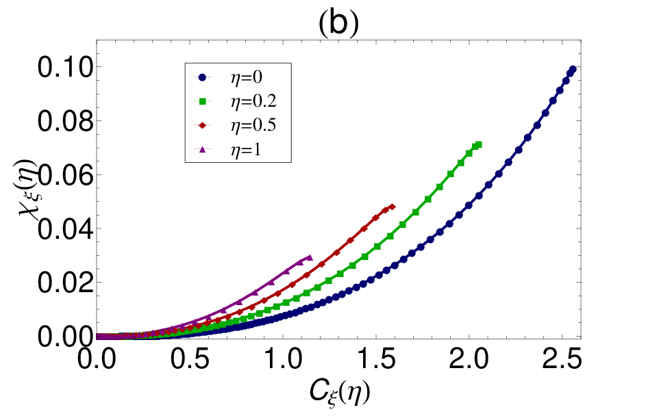
The second observation from Fig. 5 is that the maxima of are shifted to smaller values of for increasing . In Fig. 6, the values of that maximize the ratios defined in (V.1) [blue circles] and (V.2) [green rectangles] are plotted as a function of . They are almost the same. This indicates a certain relation between the formation of chiral condensates and the value of electric current correlation function in a system including relativistic fermions.

This relation is demonstrated in Figs. 7a-7c, where from (V.2) is plotted as a function of from (V.1) for fixed (or equivalently, ) and various damping parameters . Each dot in Figs. 7a-7c indicates a value of with . As it turns out, increases with increasing for a certain numbers of (see Fig. 7a). The maximum value of for which this is true, is different for different . Let us denote this specific with . For , ’s are , respectively. For , however, decreases with decreasing (see Fig. 7b). In Fig. 7c, the two curves in Fig. 7a and 7b are reassembled and demonstrate a hysteresis-like curve with increasing . However, since the LLL approximation is only valid for small and , we shall limit us to the values of for which increases with increasing (Fig. 7a).


VI Concluding Remarks
In the present paper, the effect of exponentially decaying magnetic fields on the dynamics of Dirac fermions is explored in detail. Using the Ritus eigenfunction method, we have first determined the energy spectrum of fermions in this non-uniform magnetic field and compared it with the energy spectrum of relativistic fermions in a constant magnetic field. We have then computed the chiral condensate and local electric current correlation function in the presence of strong uniform and non-uniform magnetic fields in the LLL approximation. In non-uniform magnetic fields, and depend on a dimensionless variable , which is a nontrivial function of the magnetic field’s damping parameter , the coordinate and the magnetic length . In the LLL approximation, the transverse components of the electric susceptibility, , vanish and its longitudinal component depends also on the variable , only in the presence of exponentially decaying magnetic fields. We have shown that the limits as well as are singular. In these limits, the -dependent magnetic field becomes constant, and therefore as well as arising from the -dependent magnetic field are expected to have the same value as in a constant magnetic field. But, as it turns out this is not the case. This remarkable behavior of as well as at and/or is discussed in detail in Sec. V. Let us notice that, mathematically, there is a difference between taking the limit of a quantity to zero and setting it exactly equal to zero. This difference is indeed responsible for the singular behavior of the limits and/or . When we are looking for the solution of the differential equation (II.22) for non-uniform magnetic fields, for instance, the parameter appearing in can be very small (), but it cannot be set exactly equal to zero. When , the magnetic field becomes constant, and the differential equation (II.22), leading to the solution (II.31), including associated Laguerre polynomials, has to be replaced by the differential equation (II.13) for constant magnetic fields, leading to Hermite polynomials. There is no way to reproduce the Hermite solution of the latter case from the associated Laguerre solution of the former case, by taking . This is why that although at the classical level the uniform magnetic field is reproduced in these limits from the non-uniform magnetic field, neither the energy spectrum nor the quantum corrections to as well as of the constant magnetic fields can be reproduced from their values in the non-uniform magnetic field by taking the limit .
We have also shown that for small values of and , where we believe that the LLL approximation is reliable, the ratio from (V.2) increases with increasing ratio from (V.1) up to a maximum value of , denoted by . As it turns out, the value of depends on (see Sec. V).
Let us notice that electric susceptibility (electric current correlation function) of a three-flavor color superconductor is recently computed in a strong homogeneous magnetic field in [28], and the magnetoelectric effect in a strongly magnetized quark matter is studied in detail. The present work is a second nontrivial example on the effect of external magnetic fields, in general, and spatially decaying magnetic fields, in particular, on electric current correlation function of a system containing relativistic Dirac fermions. Apart from applications in condensed matter physics, the results of this paper may also be relevant in the context of heavy ion collisions. Here, recent experimental activities at RHIC indicate the production of intense magnetic fields in the early stage of non-central heavy ion collisions [26]. Depending on the initial conditions, e.g. the energy of colliding nucleons and the corresponding impact parameters, the spatially varying magnetic fields are estimated to be in the order of Gauß, decaying very fast, within few femtometers to Gauß, and vanishing during the hadronization process [26].
VII Acknowledgments
The authors acknowledge valuable discussions with Sh. Fayazbakhsh, S. A. Jafari and A. Vaezi.
Appendix A Orthonormality relations of associated Laguerre polynomials
In this appendix, we present a number of useful orthonormality relations of associated Laguerre polynomials. To do this, let us define the integral
| (A.1) |
For , the standard orthonormality relation of associated Laguerre polynomials is given by
| (A.2) |
But, in the present paper, we have to consider the cases, where in general . To determine , we have to distinguish several cases, which are summarized in Tables 1 and 2.
The integrals for and are given by
| (A.3) |
For and , we have
| (A.4) |
The integrals for and are given by
| (A.5) |
For and , we get
| (A.6) |
References
- [1] V. C. Zhukovsky, K. G. Klimenko, V. V. Khudyakov and D. Ebert, Magnetic catalysis of parity breaking in a massive Gross-Neveu model and high-temperature superconductivity, JETP Lett. 73, 121 (2001) [Pisma Zh. Eksp. Teor. Fiz. 73, 137 (2001)], arXiv: hep-th/0012256. E. J. Ferrer, V. P. Gusynin and V. de la Incera, Magnetic field induced gap and kink behavior of thermal conductivity in cuprates, Mod. Phys. Lett. B 16, 107 (2002), arXiv: hep-ph/0101308. E. V. Gorbar, V. P. Gusynin, V. A. Miransky and I. A. Shovkovy, Dynamics in the quantum Hall effect and the phase diagram of graphene, Phys. Rev. B 78, 085437 (2008), arXiv:0806.0846 [cond-mat.mes-hall].
- [2] K. G. Klimenko and V. C. Zhukovsky, Does there arise a significant enhancement of the dynamical quark mass in a strong magnetic field?, Phys. Lett. B 665, 352 (2008), arXiv:0803.2191 [hep-ph]. A. Ayala, A. Bashir, E. Gutierrez, A. Raya and A. Sanchez, Chiral and parity symmetry breaking for planar fermions: Effects of a heat bath and uniform external magnetic field, Phys. Rev. D 82, 056011 (2010), arXiv:1007.4249 [hep-ph]. I. E. Frolov, V. C. Zhukovsky and K. G. Klimenko, Chiral density waves in quark matter within the Nambu–Jona-Lasinio model in an external magnetic field, arXiv:1007.2984 [hep-ph]. E. V. Gorbar, V. A. Miransky and I. A. Shovkovy, Chiral asymmetry and axial anomaly in magnetized relativistic matter, Phys. Lett. B 695, 354 (2011), arXiv:1009.1656 [hep-ph]. S. Fayazbakhsh and N. Sadooghi, Phase diagram of hot magnetized two-flavor color superconducting quark matter, Phys. Rev. D 83, 025026 (2011), arXiv:1009.6125 [hep-ph]; ibid., Color neutral 2SC phase of cold and dense quark matter in the presence of constant magnetic fields, ibid. 82, 045010 (2010), arXiv:1005.5022 [hep-ph]. R. Gatto and M. Ruggieri, Deconfinement and chiral symmetry restoration in a strong magnetic background, Phys. Rev. D 83, 034016 (2011), arXiv:1012.1291 [hep-ph]. V. V. Braguta, P. V. Buividovich, M. N. Chernodub and M. I. Polikarpov, Electromagnetic superconductivity of vacuum induced by strong magnetic field: numerical evidence in lattice gauge theory, arXiv:1104.3767 [hep-lat]. F. Preis, A. Rebhan and A. Schmitt, Holographic baryonic matter in a background magnetic field, arXiv:1109.6904 [hep-th]. M. N. Chernodub, J. Van Doorsselaere and H. Verschelde, Electromagnetically superconducting phase of vacuum in strong magnetic field: structure of superconductor and superfluid vortex lattices in the ground state, Phys. Rev. D 85, 045002 (2012), arXiv:1111.4401 [hep-ph]. E. S. Fraga and L. F. Palhares, Deconfinement in the presence of a strong magnetic background: an exercise within the MIT bag model, arXiv:1201.5881 [hep-ph]. S. S. Avancini, D. P. Menezes, M. B. Pinto and C. Providencia, The QCD critical end point under strong magnetic fields, arXiv:1202.5641 [hep-ph]. M. G. de Paoli and D. P. Menezes, Particle yields in heavy ion collisions and the influence of strong magnetic fields, arXiv:1203.3175 [nucl-th]. E. -M. Ilgenfritz, M. Kalinowski, M. Muller-Preussker, B. Petersson and A. Schreiber, Two-color QCD with staggered fermions at finite temperature under the influence of a magnetic field, arXiv:1203.3360 [hep-lat].
- [3] E. Elizalde, E. J. Ferrer and V. de la Incera, Neutrino propagation in a strongly magnetized medium, Phys. Rev. D 70, 043012 (2004), arXiv: hep-ph/0404234. E. J. Ferrer and V. de la Incera, Neutrino propagation and oscillations in a strong magnetic field, Int. J. Mod. Phys. A 19, 5385 (2004), arXiv: hep-ph/0408108. E. Bavarsad, M. Haghighat and R. Mohammadi, Nucleon-nucleon scattering in a strong external magnetic field and the meutrino emissivity, Phys. Rev. D 82, 105015 (2010), arXiv:1010.3906 [hep-ph]. J. Alexandre, J. Ellis and N. E. Mavromatos, On the possibility of superluminal neutrino propagation, Phys. Lett. B 706, 456 (2012), arXiv:1109.6296 [hep-ph].
- [4] K. G. Klimenko, Three-dimensional Gross-Neveu model at nonzero temperature and in an external magnetic field, Z. Phys. C 54, 323 (1992).
- [5] V. P. Gusynin, V. A. Miransky and I. A. Shovkovy, Dimensional reduction and catalysis of dynamical symmetry breaking by a magnetic field, Nucl. Phys. B462, 249 (1996), arXiv: hep-ph/9509320.
- [6] A. De Martino, L. Dell’Anna and R. Egger, Magnetic confinement of massless Dirac fermions in graphene Phys. Rev. Lett. 98, 066802 (2007), arXiv:cond-mat/0610290 [cond-mat.mes-hall].
- [7] A. Kormanyos, P. Rakyta, L. Oroszlany and J. Cserti, Bound states in inhomogeneous magnetic field in graphene: a semiclassical approach, Phys. Rev. B 78, 045430 (2008), arXiv:0805.2527 [cond-mat.mes-hall].
- [8] P. Roy, T. Kanti Ghosh, K. Bhattacharya, Localization of Dirac-like excitations in graphene in the presence of smooth inhomogeneous magnetic fields, J. Phys.: Cond. Mat. 24, 055301 (2012), arXiv:1108.1907 [cond-mat.mes-hall].
- [9] M. Ramezani Masir, P. Vasilopoulos, A. Matulis and F. M. Peeters, Direction-dependent tunneling through nanostructured magnetic barriers in graphene, Phys. Rev. B 77, 235443 (2008). P. Rakyta, L. Oroszlany, A. Kormanyos, C. J. Lambert and J. Cserti, Peculiar nature of snake states in graphene, Phys. Rev. B 77, 081403 (R) (2008), arXiv:0707.3974 [cond-mat.mes-hall]. L. Dell Anna and A. De Martino, Magnetic superlattice and finite-energy Dirac points in graphene, Phys. Rev. B 83, 155449 (2011), arXiv:1101.1918 [cond-mat.mes-hall].
- [10] E. Milpas, M. Torres and G. Murguia, Magnetic field barriers in graphene: an analytically solvable model, arXiv:1102.5298 [cond-mat.mes-hall].
- [11] K. Handrich, Quantum mechanical magnetic-field-gradient drift velocity: An analytically solvable model, Phys. Rev. B 72, 161308 (2005).
- [12] T. K. Ghosh, Exact solutions for a Dirac electron in an exponentially decaying magnetic field, J. Phys.: Cond. Mat. 21, 045505 (2009), arXiv:0911.5622 [cond-mat.mes-hall].
- [13] A. Raya, E. Reyes, Fermion condensate and vacuum current density induced by homogeneous and inhomogeneous magnetic fields in (2+1)-dimensions, Phys. Rev. D 82, 016004 (2010), arXiv:1006.2548 [hep-ph].
- [14] H. Gies and L. Roessler, Vacuum polarization tensor in inhomogeneous magnetic fields, Phys. Rev. D 84, 065035 (2011), arXiv:1107.0286 [hep-ph].
- [15] V. I. Ritus,Radiative corrections in quantum electrodynamics with intense fields and their analytical properties, Ann. Phys. 69, (1972) 555.
- [16] G. Murguia, A. Raya, A. Sanchez, E. Reyes, The electron propagator in external electromagnetic fields in lower dimensions, Am. J. Phys. 78, 700-707 (2010), arXiv:0910.1881 [hep-th].
- [17] C. N. Leung, Y. J. Ng and A. W. Ackley, Schwinger-Dyson equation approach to chiral symmetry breaking in an external magnetic field, Phys. Rev. D 54, 4181 (1996). E. J. Ferrer and V. de la Incera, Ward-Takahashi identity with external field in ladder QED, Phys. Rev. D 58, 065008 (1998), arXiv:hep-th/9803226. C. N. Leung and S. -Y. Wang, Gauge independent approach to chiral symmetry breaking in a strong magnetic field, Nucl. Phys. B 747, 266 (2006), arXiv:hep-ph/0510066.
- [18] K. Fukushima, D. E. Kharzeev, H. J. Warringa, Electric-current susceptibility and the chiral magnetic effect, Nucl. Phys. A836, 311-336 (2010), arXiv:0912.2961 [hep-ph].
- [19] C. Itzykson and J. B. Zuber, Quantum Field Theory, New York, USA: McGraw-Hill (1980).
- [20] J. S. Schwinger, On gauge invariance and vacuum polarization, Phys. Rev. 82, 664 (1951).
- [21] E. J. Ferrer and V. de la Incera, Dynamically induced Zeeman effect in massless QED, Phys. Rev. Lett. 102, 050402 (2009), arXiv:0807.4744 [hep-ph]. E. J. Ferrer and V. de la Incera, Dynamically generated anomalous magnetic moment in massless QED, Nucl. Phys. B 824, 217 (2010), arXiv:0905.1733 [hep-ph].
- [22] N. Sadooghi, Chiral MHD description of a perfect magnetized QGP using the effective NJL model in a strong magnetic field, arXiv:0905.2097 [hep-ph].
- [23] D. J. Bedingham, Dimensional regularization and Mellin summation in high temperature calculations, arXiv: hep-ph/0011012.
- [24] E. J. Ferrer, V. de la Incera and A. Sanchez, Paraelectricity in magnetized massless QED, Phys. Rev. Lett. 107, 041602 (2011), arXiv:1103.5152 [hep-ph]. E. J. Ferrer, V. de la Incera and A. Sanchez, Non-perturbative Euler-Heisenberg Lagrangian and paraelectricity in magnetized massless QED, arXiv:1204.3660 [hep-th].
- [25] N. Sadooghi and K. S. Anaraki, Improved ring potential of QED at finite temperature and in the presence of weak and strong magnetic field, Phys. Rev. D 78, 125019 (2008), arXiv:0805.0078 [hep-ph].
- [26] D. E. Kharzeev, L. D. McLerran and H. J. Warringa, The Effects of topological charge change in heavy ion collisions: ’Event by event P and CP violation’, Nucl. Phys. A803, 227 (2008), arXiv:0711.0950 [hep-ph]. V. Skokov, A. Y. Illarionov and V. Toneev, Estimate of the magnetic field strength in heavy-ion collisions, Int. J. Mod. Phys. A 24, 5925 (2009), arXiv:0907.1396 [nucl-th].
- [27] V. de la Incera, Nonperturbative physics in a magnetic field, AIP Conf. Proc. 1361, 74 (2011), arXiv:1004.4931 [hep-ph]. E. J. Ferrer, V. de la Incera, J. P. Keith, I. Portillo and P. P. Springsteen, Equation of state of a dense and magnetized fermion system, Phys. Rev. C 82, 065802 (2010), arXiv:1009.3521 [hep-ph].
- [28] B. Feng, E. J. Ferrer and V. de la Incera, Magnetoelectric effect in strongly magnetized color superconductivity, Phys. Lett. B 706, 232 (2011), arXiv:1109.3100 [nucl-th]. B. Feng, E. J. Ferrer and V. de la Incera, Photon self-energy and electric susceptibility in a magnetized three-flavor color superconductor, arXiv:1203.1630 [hep-th].