A Regularization Approach for Prediction of Edges and Node Features in Dynamic Graphs ¹¹ 1
Emile Richard : ENS Cachan - UniverSud - CMLA, France, 1000mercis, France, emile.richard@cmla.ens-cachan.fr
Andreas Argyriou : TTI Chicago, argyriou@ttic.edu
Theodoros Evgeniou : Technology Management and Decision Sciences, INSEAD Bd de Constance, Fontainebleau 77300, France, theodoros.evgeniou@insead.edu
Nicolas Vayatis : ENS Cachan - UniverSud - CMLA, UMR CNRS 8536 France nicolas.vayatis@cmla.ens-cachan.fr

We first introduce notations for the main objects of interest in the paper:

• •

  a sequence of $T$ undirected weighted graphs with $n$ vertices and their corresponding $n\times n$ adjacency matrices $A_{t}\in{\bf S}^{n}_{\geq 0},t\in\{1,2,...,T\}$, where ${\bf S}^{n}_{\geq 0}$ denotes the set of $n\times n$ symmetric matrices with nonnegative entries. We assume that, the weights of the edges are nondecreasing functions of time, which in the unweighted case means edges do not disappear but new ones may appear over time.

• •

  a multivariate time series of node features $\bigl(X_{t}\bigr)_{1\leq t\leq T}$ so that $\forall t,X_{t}\in\mathbb{R}^{n\times q}$. We denote by $X_{t}^{(i)}\in\mathbb{R}^{q}$ the $i$th row of $X_{t}$ representing the feature vector of node $i$ at time $t$. We assume that this series depends on the series of graphs via some function $\omega:\mathbb{R}^{n\times n}\to\mathbb{R}^{n\times q}$, that is, $X_{t}=\omega(A_{t})$.

Given the values of $(A_{t},X_{t})$, for $t\in\{1,2,...,T\}$, the main goal is to simultaneously predict the future value $X_{T+1}$ and the future adjacency matrix $A_{T+1}$. To this end, we introduce:

• •

  A descriptor matrix $\Phi_{t}\in\mathbb{R}^{n\times d}$, $t\in\{1,2,...,T\}$, which encodes the past information contained both in the time series $(X_{s})_{1\leq s\leq t}$ and in the sequence of adjacency matrices $(A_{s})_{1\leq s\leq t}$ into a row vector of dimension $d$ for each node.

• •

  A matrix-valued prediction function $f:\mathbb{R}^{n\times d}\to\mathbb{R}^{n\times q}$ which relates the variable $X_{t+1}$ to the past information $\Phi_{t}$ so that $X_{t+1}$ is close to $f(\Phi_{t})$. The function $f$ is unknown and has to be estimated from past data. We denote the $i$-th row component of $f$ with the notation $f^{(i)}$, $i\in\{1,2,...,n\}$. The $n$ prediction functions $f^{(i)}$ are assumed to belong to the same Hilbert space $\mathcal{H}$, equipped with the norm $\|\cdot\|_{\mathcal{H}}$. The norm of $f\in\mathcal{H}^{n}$ is defined by $\|f\|_{\mathcal{H}^{n}}:=\sqrt{\sum_{i=1}^{n}\|f^{(i)}\|^{2}_{\mathcal{H}}}$.

• •

  An unknown matrix $S\in{\bf S}^{n}_{\geq 0}$ whose elements indicate how likely it is that there is a nonzero value at the corresponding position of matrix $A_{T+1}$. The most likely edges at time $T+1$ are the ones corresponding to the largest values in $S$.

The challenge in the prediction problem on real graphs evolving over time is to relate global and slowly varying node features with local and sudden changes of edges. Thus it is reasonable to assume that the evolution of the graph is governed by unobserved latent factors [16, 15], denoted by $\Psi_{t}$, which evolve smoothly. For example, in social networks or marketing applications, latent factors could be psychological factors which account for the choices of consumers. The effect of such factors on the graph can then be measured using the adjacency matrix. For instance, the clustering coefficient captures homophilic behavior, the node degree is a good indicator of popularity and the pagerank refers to centrality and influence, the trends can be read in the evolution of node degrees and the tastes are believed to be reflected on the first singular vectors of the adjacency matrix. A possible formulation of the latent factor model sets $\Psi_{t}$ to be a pair of matrices $(U_{t},V_{t})$ governing the structure of $A_{t}$ through $A_{t}=U_{t}V_{t}^{\scriptscriptstyle\top}$, where the slow evolution of latent factors is guided by some unobserved underlying mechanism. A rigorous framework would involve a statistical model for the noise and a specific form of dependence of the matrices on their recent history. A formal example will be provided in Section 4. Both the latent factors and their evolution being unobservable, we assume that some relevant and observable features $X_{t}$ partly capture the information contained in the latent factors.

The approach studied in this paper relies on the assumption that exploiting simultaneously the structure of the graph and the dynamics of the time series should improve both prediction and graph learning. Given the information collected over the period $t=1,\ldots,T$, which is contained in the feature matrices $\Phi_{t}$, we want to learn $f$ and $S$ which satisfy the following assumptions:

• •

  [A1] Low rank. $S$ has low rank. This is a standard assumption in matrix completion problems [18, 5]. The rationale is that the factors $U_{t},V_{t}$ (see Sec. 2.2) should be of small dimension.

• •

  [A2] Graph growth regularity. The growth of the graph exhibits regularity over time, that is, $S$ should be close to the last adjacency matrix $A_{T}$. We will use the Frobenius distance between these two matrices as an estimate of the error of the learning process with respect to graph inference.

• •

  [A3] Feature growth regularity. The features of the predicted graph are assumed to be close to the predicted features. As a consequence, we assume that the norm of $f(\Phi_{T})-\omega(S)$ should be kept small.

• •

  [A4] Stationarity. The dependence mechanism between $X_{t+1}$ and $\Phi_{t}$ can be inferred. Therefore, it is reasonable to assume stationarity of the joint distribution of $(X_{t+1},\Phi_{t})$.

• •

  [A5] Regularity of the predictors over the graph. Neighboring vertices $i$ and $j$ in the graph should correspond to similar prediction functions $f^{(i)}$ and $f^{(j)}$.

We now introduce a regularization based formulation which reflects each of the previous assumptions. To this end, we introduce additional notation. For any matrix $M$, $\text{Tr}(M)$ denotes the trace of $M$ and $\|M\|_{\text{F}}:=\sqrt{\text{Tr}(M^{\scriptscriptstyle\top}M)}$ denotes the Frobenius norm of $M$. We also define $\|M\|_{*}:=\sum_{k=1}^{n}\sigma_{k}(M)$ , the nuclear norm of a matrix $M$, where $\sigma_{k}(M)$ denotes the $k$-th largest singular value of $M$. We recall that a singular value of matrix $M$ corresponds to the square root of an eigenvalue of $M^{\scriptscriptstyle\top}M$ and that the nuclear norm is a convex surrogate of the rank. We also define the matrix $\Delta(f):=\left(\|f^{(i)}-f^{(j)}\|_{\mathcal{H}}^{2}\right)_{i,j=1}^{n}$. We introduce a convex loss function $\ell:\mathbb{R}^{n\times q}\times\mathbb{R}^{n\times q}\to\mathbb{R}_{+}$ which measures prediction errors. Given the past history $\{(X_{t},A_{t})~:~1\leq t\leq T\}$, the proposed optimization problem is then to minimize over $(f,S)\in\mathcal{H}\times{\bf S}^{n}_{\geq 0}$ the following functional:

where $\lambda$, $\tau$ and $\nu$ are positive regularization parameters. Typical choices of the loss function $\ell$ are the square loss or the sum of hinge loss errors per component. Note that using different loss functions allows one to adapt the method to different problems, such as regression or classification.

We now describe each of the separate terms in the above formulation.

• •

  The first term, $J_{1}(f)=\sum_{t=1}^{T-1}\ell(f(\Phi_{t}),X_{t+1})$ $+\frac{\kappa}{2}\|f\|_{\mathcal{H}^{n}}$, corresponds to the prediction task as in standard regularized risk minimization in RKHS for supervised learning.

• •

  The second term, $J_{2}(S)=\mu\|S\|_{*}+\frac{1}{2}\|S-A_{T}\|_{\text{F}}^{2}$, with $\mu=\tau/\nu$, represents the low-rank matrix denoising objective (static link prediction) and reflects assumptions A1 and A2.

• •

  The third term, $J_{3}(f,S)=\ell(f(\Phi_{T}),\omega(S))$, penalizes the difference between the predicted features and the features of the predicted matrix. This term reflects assumption A3.

• •

  The last term, $J_{4}(f,S)=\operatorname{Tr}\bigl(S^{\scriptscriptstyle\top}\Delta(f)\bigr)$ relates the contributions of $f$ and $S$ based on assumption A.

We point out the connection of work on matrix completion [4, 12, 9] to the minimization of $\ell(f(\Phi_{T}),\omega(S))+\mu\|S\|_{*}$. Also, in [14], the authors use the minimizer $\hat{f}$ of $J_{1}$ and solve the subproblem $\operatorname*{arg\,min}_{S}J_{2}(S)+J_{3}(S,\hat{f})$.

For simplicity of presentation, we now consider the case of $\mathcal{H}$ being an RKHS corresponding to a linear kernel. In addition, each $f^{(i)}$ is a linear function represented by a $d\times q$ matrix $W^{(i)}$, so that $f^{(i)}(\Phi_{t})=\Phi^{(i)}_{t}W^{(i)}$. Then we may assume $\|f^{(i)}\|_{\mathcal{H}}=\|W^{(i)}\|_{F}$ and the graph regularity term can be expressed in terms of the graph Laplacian of $S$. Recall that the Laplacian is defined as the operator $\Lambda$ such that $\Lambda(S)=D-S$ where $D=\operatorname{diag}(d_{1},\ldots,d_{n})$ and $d_{i}=\sum_{j=1}^{n}S_{ij}$ are the degrees of the graph. A standard computation gives the following expression for $J_{4}$:

where $W=(W^{(1)},\ldots,W^{(n)})\in\mathbb{R}^{n\times d\times q}$. We use the standard extension of the Frobenius norm to 3-tensors, $\|W\|_{F}^{2}=\sqrt{\sum_{i=1}^{n}\|W^{(i)}\|^{2}_{F}}$ and the notations:

We also assume in this work that the node features are linear functions of adjacency matrices : $\omega(A_{t})=A_{t}\Omega$ for some $\Omega\in\mathbb{R}^{n\times q}$. Note that degree, inter/intra cluster degrees and projection onto specific linear subspaces are such features, but not clustering coefficients or statistics on path lengths. We later detail how we chose $\Omega$ in our experiments.

In the experiments conducted, we have learned linear functions $f^{(i)}$. In this case, the term $\sum_{1\leq i,j\leq n}S_{ij}\|W^{(i)}-W^{(i)}\|_{F}^{2}$ is convex with respect to one of the variables, if the other is fixed, but not jointly convex with respect to $(W,S)$. In order to ensure convergence of an optimization algorithm to a desired minimum, we determine a domain where $\mathcal{L}$ is convex. We use intuition from what happens with a similar optimization problem in dimension 2. Indeed, consider the minimization of $(w,s)\rightarrow sw^{2}+\alpha s^{2}+\beta w^{2}$ which is the simplified functional in the degenerate case where $n=1$. The eigenvectors of the Hessian are positive iff $w^{2}\leq\alpha\beta$, so this condition defines the convexity region. By adding the quadratic terms in $S$ and $W$ to $Q(W,\Lambda(S),W)$, let us define

If we suppose that the entries of $Z=S-A_{T}$ are nonnegative, then the minimizer of $\Psi$ is the trivial solution $S=A_{T},W=0$. In fact,

and for $Z=0,W=0$, $\Psi(S,W)=0$.

We prove that $\mathcal{L}$ is convex over a set $\mathcal{E}$ around the minimizer of $\Psi$ and we will ensure henceforth that the descent algorithm takes place inside this convex domain.

Letting $z=\|Z\|_{F},w=\|W\|_{F},w_{0}=\|W_{0}\|_{F}$, we have

$\psi_{w_{0}}:(z,w)\mapsto\frac{\nu}{2}z^{2}+\frac{\kappa}{2}w^{2}-2\lambda(\sqrt{n}+1)wzw_{0}$ is a quadratic form. Therefore $R(Z,W)$ is always nonnegative if $\psi_{w_{0}}$ is positive semidefinite positive. That is, if $\nu+\kappa\geq 0$ (always true) and $\nu\kappa-4\lambda^{2}\bigl(\sqrt{n}+1\bigr)^{2}w_{0}^{2}\geq 0$, and this completes the proof.

For optimization purposes, we chose to replace the nonsmooth nuclear norm term by a smooth approximation, in the spirit of the optimization literature, for example [13],

Each of these parameterized functions is a lower bound that approaches $\|S\|_{*}$ as $\eta\to 0^{+}$, while being differentiable. Differentiability is due to $-g_{\eta}$ being related to a Moreau envelope [11] and specifically to the squared distance of $\frac{1}{\eta}S$ from the unit ball of the spectral norm.

In the case of a differentiable loss $\ell$, we explicitly compute $\nabla\mathcal{L}(W,S)$ as

and

where $S=U(S)\text{Diag}\bigl(\sigma_{1}(S),\ldots,\sigma_{n}(S)\bigr)V(S)^{\scriptscriptstyle\top}$ is a singular value decomposition of $S$. In the case of squared loss,

Therefore:

We recall that our setup consists of a regression-type model for the prediction of $(X_{T+1},A_{T+1})$ given the available information at time $T$ which includes the previous adjacency matrices $A_{1},\ldots,A_{T}$ of size $n\times n$ and the node-related feature matrices $X_{1},\ldots,X_{T}$ of size $n\times q$. Our approach involves a $\Phi_{T}$ of size $n\times d$ called descriptor matrix which encompasses the information contained in the past realizations $(X_{t},A_{t})$ for $t\leq T$.

Various prediction tasks could be studied in our setup with specific criteria for optimization and evaluation. We focus here on regression (for feature prediction) and graph completion (for link prediction), but classification of vertices may also be a useful task.

Since the problem which we address (simultaneous graph completion and feature prediction) is a novel one, there are no direct competing methods to compare with. Thus, in our experiments we have considered the following baselines which address the most similar learning problems:

1. 1.

   Ridge Regression. Learning the function $\hat{f}:=\operatorname*{arg\,min}_{\mathcal{H}}J_{1}$ through the minimization of the penalized regression $J_{1}(f)=\sum_{t=1}^{T-1}\ell(f(\Phi_{t}),X_{t+1})+\frac{\kappa}{2}\|f\|_{\mathcal{H}^{n}}^{2}$ leads us to a prediction function $\hat{f}$ which we use for predicting $X_{T+1}$ by $f(\Phi_{T})$. This approach addresses the prediction of node features as independent time series. It does not take the graph sequence into account and does not predict the future graph.

2. 2.

   Rank-free prediction. We used our formulation with the choice of $\tau=0$. In this case, the loss function ignores the low-rank hypothesis in the graph structure. The prediction process only relies on the dynamics of graph features.

3. 3.

   Graph completion through shrinkage. We also considered a method only dedicated to link prediction and matrix denoising, ignoring the feature prediction part of the problem. This method only uses the observation $A_{T}$ as a noisy version of $A_{T+1}$, and aims at predicting $A_{T+1}$ given only this observation and the low rank hypothesis. We solve the problem $\min_{S}J_{2}(S)$ where $J_{2}(S)=\frac{1}{2}\|S-A_{T}\|_{F}^{2}+\mu\|S\|_{*}$ to estimate the adjacency matrix as a low rank approximation of $A_{T}$. The solution of this problem is obtained by singular value shrinkage [4], namely if $A_{T}=U\operatorname{diag}{(\sigma_{1}(A_{T}),\ldots,\sigma_{n}(A_{T}))}V^{\scriptscriptstyle\top}$ is the singular value decomposition of $A_{T}$, then the image of $A_{T}$ by a shrinkage of parameter $\mu$ is given by $D_{\mu}(A_{T})=U\operatorname{diag}{(\sigma_{i}(A_{T})-\mu)_{+}}V^{\scriptscriptstyle\top}$ .

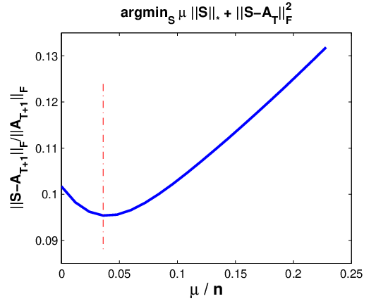
We implemented a first-order gradient descent algorithm with projections on the convex set $\mathcal{E}$ at each iteration. In Figure 2 we show how cross validation can be done first on the two standard objectives of regression and graph completion (matrix denoising) taken separately for setting the values of $\mu=\frac{\tau}{\nu}$ and $\kappa$ efficiently. This reduces the number of smoothing parameters, and thanks to experiments on synthetic data we studied the dependence of optimal regularization parameters $\kappa,\tau,\nu,\lambda$ on the model parameters $r,\sigma,\epsilon$. We illustrate in Figure 3 the efficiency of our algorithm for minimizing different objective terms despite competing effects at the starting point of optimization. We emphasize the decrease of validation error as a function of the number of iterations. Finally, in Figure 4, we report results of experiments on marketing data sets, which show that, with appropriately chosen hyperparameters, our approach outperforms standard competing baselines. We also observe that on the top-selling items data set, the nuclear norm term does not add to prediction accuracy compared to the rank-free $\tau=0$ case. Further study is needed to better understand whether this effect is due to the possible presense of high noise or to the higher efficiency of predicted features in predicting the future graph.

References

- [1] Jake Abernethy, Francis Bach, Theodoros Evgeniou, and Jean-Philippe Vert. A new approach to collaborative filtering: operator estimation with spectral regularization. JMLR, 10:803–826, 2009.
- [2] Andreas Argyriou, Massimiliano Pontil, Charles Micchelli, and Yiming Ying. A spectral regularization framework for multi-task structure learning. Proceedings of Neural Information Processing Systems (NIPS), 2007.
- [3] Leo Breiman and Jerome H. Friedman. Predicting multivariate responses in multiple linear regression. Journal of the Royal Statistical Society (JRSS): Series B (Statistical Methodology), 59:3–54, 1997.
- [4] Emmanuel J. Candès and Terence Tao. A singular value thresholding algorithm for matrix completion. SIAM Journal on Optimization, 20(4):1956–1982, 2008.
- [5] Emmanuel J. Candès and Terence Tao. The power of convex relaxation: Near-optimal matrix completion. IEEE Transactions on Information Theory, 56(5), 2009.
- [6] Xi Chen, Seyoung Kim, Qihang Lin, Jaime G. Carbonell, and Eric P. Xing. Graph-structured multi-task regression and an efficient optimization method for general fused lasso. arXiv, 2010.
- [7] Theodoros Evgeniou, Charles A. Micchelli, and Massimiliano Pontil. Learning multiple tasks with kernel methods. Journal of Machine Learning Research, 6:615–637, 2005.
- [8] Mladen Kolar and Eric P. Xing. On time varying undirected graphs. in Proceedings of the 14th International Conference on Artifical Intelligence and Statistics AISTATS, 2011.
- [9] Vladimir Koltchinskii, Karim Lounici, and Alexandre Tsybakov. Nuclear norm penalization and optimal rates for noisy matrix completion. Annals of Statistics, 2011.
- [10] David Liben-Nowell and Jon Kleinberg. The link-prediction problem for social networks. Journal of the American Society for Information Science and Technology, 58(7):1019–1031, 2007.
- [11] Jean-Jacques Moreau. Proximité et dualité dans un espace hilbertien. Bulletin de la Société Mathématique de France, 93(2):273–299, 1965.
- [12] Sahand Negahban and Martin J. Wainwright. Estimation of (near) low-rank matrices with noise and high-dimensional scaling. Annals of Statistics, 39:1069–1097, 2011.
- [13] Yurii Nesterov. Smooth minimization of non-smooth functions. Mathematical Programming, 103(1):127–152, 2005.
- [14] Emile Richard, Nicolas Baskiotis, Theodoros Evgeniou, and Nicolas Vayatis. Link discovery using graph feature tracking. Proceedings of Neural Information Processing Systems (NIPS), 2010.
- [15] Purnamrita Sarkar, Deepayan Chakrabarti, and Andrew W. Moore. Theoretical justifiation of popular link prediction heuristics. In Proceedings of COLT, 2010.
- [16] Purnamrita Sarkar and Andrew Moore. Dynamic social network analysis using latent space models. In Y. Weiss, B. Schölkopf, and J. Platt, editors, Proceedings of Neural Information Processing Systems 18, pages 1145–1152. MIT Press, Cambridge, MA, 2006.
- [17] Ashish Sood, Gareth M. James, and Gerard J. Tellis. Functional regression: A new model for predicting market penetration of new products. Marketing Science, 28(1):36–51, 2009.
- [18] Nathan Srebro, Jason D. M. Rennie, and Tommi S. Jaakkola. Maximum-margin matrix factorization. In Lawrence K. Saul, Yair Weiss, and Léon Bottou, editors, in Proceedings of Neural Information Processing Systems 17, pages 1329–1336. MIT Press, Cambridge, MA, 2005.
- [19] Ruey S. Tsay. Analysis of Financial Time Series. Wiley-Interscience; 3rd edition, 2005.
- [20] Ducan J. Watts and Steven H. Strogatz. Collective dynamics of small-world networks. Nature, 393:440–442, 1998.