Glassy Critical Points and the Random Field Ising Model
Abstract
We consider the critical properties of points of continuous glass transition as one can find in liquids in presence of constraints or in liquids in porous media. Through a one loop analysis we show that the critical Replica Field Theory describing these points can be mapped in the -Random Field Ising Model. We confirm our analysis studying the finite size scaling of the -spin model defined on sparse random graph, where a fraction of variables is frozen such that the phase transition is of a continuous kind.
pacs
05.20.-y, 75.10NrI Introduction
The last years of research have emphasized the importance of fluctuations in understanding glassy phenomena. The present comprehension of long lived dynamical heterogeneities in supercooled liquids compares the growth of their typical size to the appearance of long range correlations at second order phase transition points [1]. Unfortunately, in supercooled liquids, the theoretical study of these correlations beyond the Mean Field is just at an embryonic level. It has been recently proposed that the putative discontinuous dynamical transition of Mode Coupling Theory, which is present when all activated processes are neglected, belongs to the universality class of the unstable theory in a random field (-RFIM in the following) [2]. However in real systems the activated processes cannot be neglected, the only remnant of the transition is a dynamical crossover and it is not clear if there is a range where the prediction of the theory can be tested.
In usual phase transition often we have a line of first order transitions that ends at a second order terminal critical point. The most popular case are ferromagnets: at low temperatures there is a first order transition when the magnetic field crosses zero (the magnetization has a discontinuity) and this transition lines end at the usual critical point. The same phenomenon happen for the gas liquid transition: it is a first order transition at low temperatures that ends in a second order transition at the critical point.
A similar situation can occur for liquids undergoing a glass transition, where lines of discontinuous glass transitions can terminate in critical points. In this note we focus our attention to these terminal points, where the glass transition becomes continuous and activation does not play a major role in establishing equilibrium. This transition has both a dynamic and a thermodynamic character, and it is not necessarily wiped out in finite dimension. Glassy critical points have been theoretically studied in detail both at the dynamic and at the thermodynamic level. In dynamical Mode Coupling Theory (MCT)[3] these are known as singularities, and have been recently observed in simulations of kinetically constrained models on Bethe lattice [4]. At the thermodynamic level they are known from mean field Spin Glass models [5] and Integral Equations approximations of liquid theory [6]. At these points the discontinuity in the Edwards-Anderson non-ergodicity parameter vanishes and correspondingly, the separation of dynamics in alpha and beta regime is blurred. On approaching the critical points from the discontinuous transition side the MCT exponents characterizing the beta relaxation go to zero and the alpha relaxation follows a universal scaling function [7]. In general bulk liquids display a discontinuous transition pattern. However, the transition can become continuous for a particular choice of the parameters, e.g. in presence of constraints or of quenched disorder. It has been argued that within MCT the glass transition can become continuous for liquids are confined in porous media [8]. If one studies the transition as a function of the spatial density of the confining matrix , one finds lines of discontinuous dynamic and thermodynamic transition that get displaced at lower and lower liquid densities, until they merge at a common critical point where the transition becomes continuous.
From the theoretical side a suitable way of constraining a glassy system consists in introducing a “pinning field” term in the Hamiltonian pushing the system in the direction of a randomly chosen reference equilibrium configuration. In [9] it was proposed a phase diagram in the plane of temperature and pinning field, showing lines of first order dynamical and thermodynamical transition that merge and terminate in a common critical point as reproduced in figure 1. This view, based on simple spin glass models, was confirmed for liquids in the replica hypernetted chain approximation in [10] and supported by numerical simulation of realistic model liquids in [11, 10].
More recently, the interest for the phase diagram of constrained systems has been renewed by liquid simulations where a finite fraction of the particles are frozen to the position they take in a selected equilibrium configuration[12]. The effect of the frozen particles is similar to the one of an adsorbing matrix in a porous medium or of a pinning field, with the important addition that in this case the unfrozen particles remain in the original equilibrium state.
The detailed phase diagram for spin models on random graphs was computed in [13, 14]. A theoretical discussion of the physical relevance of this situation for liquids and glasses and an exact computation for the mean field -spin models were presented in [15]. Differently from the case of the pinning field where the field transforms the glass transition into first order and spinodal transitions, in the case of frozen particles the dynamic and thermodynamic transition lines keep with their glassy random first order character that one finds at zero pinning.
In all these cases, the existence of a critical terminal point is interesting because while the dynamical critical line has to disappear in finite dimension thanks to dynamical activation, the critical terminal point, which is also the terminating point of the thermodynamic transition line could survive in finite dimensions and can be studied in numerical simulations and experiments.
As it is usual for lines of phase transitions terminating in a critical point, the critical terminal point lies in a different universality class of the line. The critical properties of discontinuous dynamical transitions has been recently analyzed in [2]. It has been proposed that the time independent part of the fluctuations in the and early dynamical regimes admit a description in terms of a cubic replica field theory. The leading singularities of this theory in perturbation theory happen to coincide with the ones of a field theory in a random magnetic field. At the critical point the coefficient of the term vanishes and it is natural to make the hypothesis that the next relevant term is a term so that the resulting theory is the standard -RFIM [16].
Arguments in this direction have been put forward in [15] using a RG procedure. Unfortunately, the arguments in [15], though suggestive, are not fully convincing. They are based on a Migdal-Kadanoff renormalization scheme, which uses a hybrid formalism where replicas are used to average out the randomness in couplings, but additional quenched disorder introduced to mimics the effect of the frozen particle is kept unaveraged.
In this paper we use the tools of replica field theory to support the hypothesis that glassy critical points are in the universality class of the -RFIM. We analyze in detail the case of a dynamical transition line terminating in a critical point. Such a scenario applies exactly in the case in which a finite fraction of particles are pinned in an equilibrium condition. The case of a pinning field or of an adsorbing matrix presents additional complications that will be left to future work. Replica field theory can be used to find out the nature of this transition. We have to consider a system with clone in presence of some constraint: when the number of components goes to 1, one of the clones is at equilibrium and the other clones feel the effect of a quenched field. Since one does not specify which of the clones is privileged the final theory is replica symmetric. From a field theoretical perspective, at first site the RFIM hypothesis is self-evident: indeed if we take care of the leading terms, the replica theory corresponds to theory with a random temperature, that maps on a theory with a potential with a random magnetic field and the critical terminal point is described by a interaction. However this argument holds only for the leading terms and neglects sub-leading orders that may play a crucial role if the leading terms cancels.
More precisely the mapping of the dynamical transition to the -RFIM comes from the extraction of the most singular contribution of a cubic replica field theory, with multiple fields of different scaling dimension. The neglected sub-leading terms turn out to become dimensionally relevant below dimension 6, the same dimension as the quartic terms of the -RFIM. The contribution of cubic vertexes cannot therefore be directly dismissed on the basis of dimensional analysis. To understand the nature of the terminal critical point and the possibility of cancellations that restore the RFIM mapping, a careful analysis of the perturbative series is needed. The scope of this note is to investigate this problem at the level of Ginzburg criterion, computing the one loop corrections to the propagators due to the residual cubic vertexes and comparing them to the ones coming from the quartic terms. We find that a-priori unexpected cancellations are present so that the cubic vertexes contributions appear to be irrelevant as compared to the quartic ones.
In order to test our theoretical results, we consider a diluted -spin model (random XOR-SAT problem) on a random graph in presence of frozen spins and perform extensive numerical simulations to study finite size scaling close to the critical point. The simulations on large systems fully confirm our analysis, making us confident that the one-loop result indeed holds to all orders.
In the next section we present the theoretical analysis. In the subsequent one the numerical simulation. We then conclude the paper. An appendix is devoted to the technical details of the theoretical computations.
II Analysis
Our starting point is the replica field theory [17, 18]
| (1) |
where the field is an space dependent matrix order parameter with vanishing diagonal terms, describing the fluctuations of the correlation function around its plateau value. Among all possible cubic replica invariant we have retained only the ones giving rise to the leading and possible next to leading singular behavior. It has been show in [2] that in the limit the theory describe fluctuations close to the dynamical transition, that occurs for (while and remain finite).
According to the discussion in [2] the components of the matrix do not share a unique scaling dimension. Similarly to what found in the RFIM problem [19], in order to use dimensional analysis one needs to change basis and define linear combinations , and of the that exhibit good scaling properties. The actual linear transformation reeds
| (2) |
where is a size two band matrix and is a symmetric matrix null on the diagonal and such that
| (3) |
The analysis of the resulting quadratic form (see below) shows that , and have well defined scaling dimension , and that, fixing the dimension , verify and . Fixing the dimension of by the condition that the action is adimensional one finds . Notice that if the normalization of the dimension would be fixed by the condition that the dimension of the momentum is one, we should multiply all dimensions by a factor two.
In terms of the new fields, keeping only the terms giving rise to the leading singularities in perturbation theory and sending , one finds that (1) is equivalent to the Parisi-Sourlas action [20]
| (4) |
where the matrix of fields has independent components. These fields enter quadratically in (4). Explicit integration over them gives rise to a determinant to the power that tends to for and is equivalent to the one generated by fermion fields. The cubic vertex has a coupling constant , it has scaling dimension and becomes relevant below dimension 8.
In different systems the various parameters appearing in the action are function of the physical control parameters e.g. temperature and pinning field amplitude, or fraction of blocked particles. At the critical point one has , the cubic coupling constant is equal to zero and sub-leading singular vertexes need to be considered in the Landau free-energy expansion. We should therefore consider quartic terms and sub-leading cubic ones. Dimensional analysis, through repeated use of (2), shows that among all possible quartic replica symmetric invariants, the most singular ones are11 1 We thank T. Rizzo and L. Leuzzi for pointing us a contribution previously neglected.
| (5) |
that after the change of basis the leading terms (lowest scaling dimension) give rise to the RFIM terms
| (6) |
The scaling dimension of this vertex is which thus becomes relevant below 6 dimension. In addition one needs in principle to consider the cubic vertexes that do not vanish for . Among these, the ones of higher scaling dimension are and , which for give rise to the term . This term does not have evident reasons to vanish. Its superficial scaling dimension (when multiplied by ) is and in absence of additional cancellations is would also become relevant below 6 dimensions. The relevance of these vertexes would spoil the equivalence with the RFIM at the critical point.
In order to investigate the possible relevance of these terms in the action we could in principle analyze their contribution to the correlation functions of the various fields in perturbation theory. To do this one needs to keep into account the constraints (3) which give rise to some cumbersome combinatorics.
We have preferred therefore to turn back to the original replica field theory (1) and compute the exact contribution of the cubic vertexes to the self-energy and to the correlation functions to the one loop level. The diagrams contributing to the self-energy of a generic cubic theory are depicted in fig. 2, they are the diagrams irreducible against cuts that separate the ending points [21].

The structure of the bare propagator of the theory in momentum space induced by replica symmetry is
| (7) |
where the three coefficients , can be expressed as function of the mass parameters appearing in the action (1), in the limit :
| (8) | |||
| (9) | |||
| (10) |
Notice that while and have a simple pole behavior for small and , has a double pole.
Given the structure of the propagator and the vertexes, the direct manual evaluation of the self-energy diagrams to include the sub-leading order is rather awkward. The formal expression of the diagrams of fig. 2 is given in the appendix. Fortunately, the computation of the diagrams, which basically involves sums of constants and delta functions over replica indexes and momentum integration, can be fully automatized. We have achieved this goal using the algebraic manipulator Mathematica, defining functions that implement the Kronecker delta on the one hand and the sum of constants and delta functions on the other. In order to compute the contribution to the correlation function one needs to further multiply the resulting expression to the right and to the left by the bare propagator, which can also be done by automatic means.
The result for the corrections to the correlation function can be cast in a form similar to the one of the bare propagator (7), parametrized by three numbers analogous to the ’s of (7). The resulting expressions, available upon request, are rather lengthy and we do not reproduce them here. For the leading singularity behaves as , with corrective terms of order and higher. Comparing the leading contribution with the behavior of the bare propagator one sees that, as already found with the -RFIM mapping of [2], non Gaussian fluctuations become important below dimension 8. For the leading terms vanish. Remarkably the computation shows that at the same time the corrective terms of order , also vanish. In fact these contributions are proportional to . The first non vanishing contributions are of order . These are irrelevant down to dimension 4, as opposed to the quartic RFIM contribution which become relevant in dimension 6.
This result proves the -RFIM mapping to the one loop order in perturbation theory. Though we believe the result to be valid to all orders the general mechanism for cancellation of the contribution of the cubic vertexes remains to be found. It would be tempting to think that for the fields in (2) verify fermionic algebraical relations that go beyond the simple identification of the replica determinant with the fermionic one that was used in [2].
III Simulations
In order to check whether the universality class of the terminal critical point is that of a -RFIM we have simulated the 3-spin model on a random regular graph with fixed degree . The Hamiltonian of the model is
where are Ising variables and the indexes are randomly chosen such that each variable appears exactly times and each interaction involves 3 different variables. The couplings are independent random binary variables, generated according to and . In the thermodynamical limit, the model has been solved with the cavity method [22] and presents a dynamical phase transition at a temperature [2], followed by Kauzmann ideal glass transition at a lower temperature . As long as , the thermodynamical and dynamical properties of the model do not depend on the choice of the coupling bias , because almost any coupling configuration has the same free energy, thanks to the fact that the annealed average equals the quenched one (). In particular we can choose the couplings according to the Nishimori prescription [23] that corresponds to . This choice has the great advantage that the all-spin-up configuration is an equilibrium configuration and we can use it as the starting configuration for the study of the equilibrium dynamics and also as the initial configuration for a Monte Carlo simulation, which does not require thermalization [24].
III.1 Phase diagram with frozen variables
We are interested in studying the 3-spin model defined above, when a fraction of variables are frozen to an equilibrium configuration (the all-spin-up configuration in the present case). The phase diagram in the plane resembles closely the one derived in [13, 14] for the 3-XORSAT model 22 2 The 3-XORSAT model is nothing but the 3-spin model on a random graph of mean degree at . Phase transitions takes place varying , which plays the same role of the temperature in thermal models. in the plane (see Fig.3 in [14]). It is also very similar to the one derived in [15] for the spherical 3-spin model.
In Fig. 3 we show the numerical data for the dynamical critical temperatures as a function of obtained by the cavity method. All the critical points shown (but the terminal point that we discuss in the following) as been obtained by looking at the overlap with the reference equilibrium configuration (): the dynamical critical temperature corresponds to the negative jump in this overlap when the temperature is slowly increased.
A much more careful discussion requires the determination of the terminal critical point, that we estimate to be located in and . Indeed at the terminal critical point the phase transition is no longer of first order and there is no jump in the overlap with the reference configuration to be exploited (even for but close to the terminal point the jump is so small that is not useful to estimate the transition location). On the contrary, for the model has no phase transition at all and one can at most look at the precursors of the continuous phase transition taking place at the terminal critical point.
The problem of locating the terminal critical point with high accuracy is delicate and we have followed a method based on solving the cavity equations in population, while looking at the instability parameter . More precisely, we run the Belief Propagation (BP) algorithm for determining the fixed point distribution of cavity magnetizations that solves the equation
where . Then we have computed the local stability of the fixed point distribution by adding a small perturbation to each element of the population and checking whether such a perturbation grows or decreases under BP iterations: the stability parameter is defined such that the perturbation goes like for large times . So the fixed point is stable only if . In a discontinuous transition the condition identifies the spinodal points where the two states becomes locally unstable; while in a continuous transition the condition marks the unique critical point.
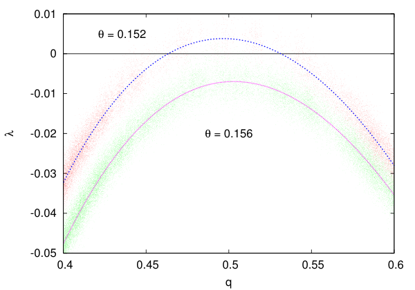
In Fig. 4 we show the stability parameter as a function of the overlap with the equilibrium reference configuration. For each value of , the plot contains few tens of thousands of points measured at different temperatures around the critical one (both above and below the critical temperature). The noise in the data is due to the stochastic nature of the BP algorithm and to fluctuations related to the finiteness of the population (we have used populations of sizes ). It is worth stressing that mainly depends on , while its dependence on the temperature is rather weak: indeed Fig. 4 shows data measured at different temperatures that lay on the same curve. The interpolating curves shown in Fig. 4 are quartic polynomials.
For the model undergoes a discontinuous phase transition: the two values for which bracket an interval where no state can exist in the thermodynamical limit (since it would be locally unstable); by varying the temperature, the thermodynamic overlap has a jump not smaller than the size of this interval. Moreover the larger overlap where is the plateau value at the dynamical critical temperature . For the stability parameter never becomes positive and consequently the model has a unique paramagnetic phase and no phase transition. The value of the terminal critical point is clearly in between these two values and for the function must have a maximum of height . The quartic interpolations shown in Fig. 4 allow us to obtain reliable estimate of position and height of the maximum of the function for each value. Fitting these maxima we then arrive at the following estimates for the terminal critical point: and .
A reliable way to estimate the temperature of the terminal critical point is by plotting the average overlap as a function of the temperature for values at and around (see Fig. 5). In this way we can estimate as the temperature at which the average overlap measured at reaches the critical value . The uncertainty on this value comes both form the statistical error in this fitting procedure and from the propagation of the uncertainty on the value . In Fig. 5 we plot data for several values such that one can appreciate how much the average overlap changes by varying . The final estimate for the temperature of the terminal critical point is . The error is mainly given by the uncertainty on the value of .
III.2 Fluctuations at the terminal critical point
Once we have obtained a reliable estimate for the location of the terminal critical point, and , we have run extensive Monte Carlo simulations for those critical parameters. We have simulated sizes up to . For each size, but the largest, we have simulated different samples (for the largest size only 2500 samples were used). Thermalization is not an issue, given that the all-spin-up configuration is an equilibrium configuration by construction.
As already discussed in detail in [2], there are 3 different sources of randomness in this model: the coupling configuration, the starting equilibrium spin configuration and the thermal noise. Thanks to the fact the annealed approximation is exact in this model above , in the thermodynamical limit every sample behaves exactly the same, when the average over starting configurations and thermal noise is performed. However, we do not take the average over many initial spin configurations, and we only use as the starting configuration to avoid thermalization. So, the average over the many coupling configurations we consider does actually correspond to the average over the initial spin configurations: indeed we could gauge transform each sample in order to have roughly the same couplings and the initial spin configuration would change from sample to sample.
So, we are left we only 2 sources of randomness: heterogeneities in the initial configuration (het) and thermal noise (th). Using the angular brackets for the thermal average and the square brackets for the average over the initial spin configurations, two different susceptibilities can be defined as follows
| (11) | |||||
| (12) |
where the former measures thermal fluctuations within the same sample (averaged over the samples), while the latter quantifies sample to sample fluctuations in the mean value of (which is as usual the overlap with the equilibrium reference configuration). The total susceptibility is the sum of the two: .
A dimensional analysis of action of the -RFIM leads straightforwardly to the following scaling relations for the susceptibilities
| (13) | |||||
| (14) |
In Fig. 6 we show the data collapse using the theoretically predicted exponents. We can see that the scaling for the largest fluctuations, , is very well verified, while some corrections to the scaling are still present in the data for the thermal fluctuations at the sizes we have simulated.
IV Summary
Summarizing, we have found that Replica Field Theory of glasses predicts that fluctuations close to glassy critical points can be mapped into the Random Field Ising Model. This observation calls for the search of glassy critical points in liquid systems. In simulations one can use the method of pinning field or blocking a fraction of the particles. In experiments critical points could be found in liquids confined by porous media.
Acknowledgments
We thank G.Biroli, C.Cammarota, L. Leuzzi, T. Rizzo and P. Urbani for discussions. SF acknowledges the physics department of Rome university “Sapienza” for hospitality. F. R.-T. acknowledges the LPTMS, Université Paris-Sud 11 for hospitality. The European Research Council has provided financial support through ERC grant agreement no. 247328.
V Appendix
This appendix is devoted to the explanation of some technical details of the evaluation of the one loop corrections to the propagator.
The diagrams that we need to evaluate are conceptually simple, but practically complicated by the presence of the replica indexes in the propagator and the vertexes that we write as:
| (15) |
| (16) |
where denotes symmetrization against exchange of indexes in each couple and and exchange of the couples among themselves. The first self-energy diagram reads
| (19) | |||||
the second one is
| (21) | |||||
In order to compute the correction to the propagator the one loop self-energy should be multiplied to the right and to the left by the bare propagator.
| (22) |
The whole calculation involves sums of constants and delta functions over replica indexes. In order to avoid mistakes we have automatized the calculation through the use of the software Mathematica. We reproduce here the commented worksheet used in the calculation.
References
- [1] Dynamical heterogeneity in glasses, colloids and granular media L. Berthier, G. Biroli, J.-P. Bouchaud, L. Cipelletti, and W. van Saarloos eds. Oxford University Press (2011)
- [2] S. Franz, F. Ricci-Tersenghi, T. Rizzo, G. Parisi Eur. Phys. J. E 34 9 (2011) 102 and arXiv:1105.5230.
- [3] See e.g. W. Götze Complex Dynamics of glass forming liquids. A mode-coupling theory. Oxford: Oxford University Press. 2009.
- [4] M. Sellitto, D. De Martino, F. Caccioli, and J. J. Arenzon PRL 105, 265704 (2010), M. Sellitto Phys. Rev. E 86, 030502(R) (2012)
- [5] A. Crisanti and H.-J. Sommers, Z. Phys. B 87 (1992) 341
- [6] V. Krakoviack Phys. Rev. E 82, 061501 (2010)
- [7] S. Franz, G. Parisi, F. Ricci-Tersenghi, T. Rizzo and P. Urbani arXiv:1211.1616
- [8] V. Krakoviack Phys. Rev. Lett. 94, 065703 (2005), Phys. Rev. E 84, 050501(R) (2011)
- [9] S. Franz and G. Parisi, Phys. Rev. Lett. 79 (1997) 2486
- [10] M. Cardenas, S. Franz and G. Parisi, J.Phys. A: Math. Gen. 31 (1998) L163, J. Chem. Phys. 110 (1999) 1726.
- [11] S. Franz and G. Parisi, Physica A 261 (1998) 317.
- [12] L. Berthier, W. Kob, Phys. Rev. E 85 (2012) 011102.
- [13] Solving Constraint Satisfaction Problems through Belief Propagation-guided decimation, A. Montanari, F. Ricci-Tersenghi and G. Semerjian, Proceedings of the 45th Annual Allerton Conference on Communication, Control, and Computing (Monticello, IL, USA), 352 (2007).
- [14] F. Ricci-Tersenghi and G. Semerjian, J. Stat. Mech. P09001 (2009).
- [15] G. Biroli and C. Cammarota, PNAS 109 8850 (2012) and arXiv:1210.8399.
- [16] For a review, see T. Nattermann, Spin glasses and random fields (World scientific, Singapore, 1998), p. 277.
- [17] T. Temesvari, C. De Dominicis and I. R. Pimentel, Eur. Phys. J. B 25, 361 (2002)
- [18] M. Campellone, G. Parisi and P. Ranieri, Phys. Rev. B 59. 1036 (1999).
- [19] J. Cardy, Phys. Lett. 125B, 470, 1983; Physica 15D, 123, 1985.
- [20] G. Parisi, N. Sourlas. Phys. Rev. Lett. , 43 (1979) 744.
- [21] S. Coleman and S. Glashow, Phys. Rev. 134 b671 (1964),
- [22] F. Ricci-Tersenghi and A. Montanari, Phys. Rev. B 70, 134406 (2004).
- [23] H. Nishimori, J. Phys. C: Solid State Phys. 13, 4071 (1980)
- [24] F. Krzakala and L. Zdeborova J. Chem. Phys. 134, 034512 (2011); J. Chem. Phys. 134, 034513 (2011)
Mathematica worksheet See pages - of print1.pdf