St. John’s College
\universityUniversity of Cambridge
\crest
\degreeDoctor of Philosophy
\degreedateSeptember 2011
Dynamical instabilities in disc-planet interactions
Abstract
Protoplanetary discs can be dynamically unstable due to
structure induced by an embedded giant planet. In this thesis, I
discuss the stability of such systems and explore the consequence of
instability on planetary migration.
I present semi-analytical models to understand the formation of the unstable structure induced by a Saturn mass planet, which leads to vortex formation. I then investigate the effect of such vortices on the migration of a Saturn-mass planet using hydrodynamic simulations. I explain the resulting non-monotonic behaviour in the framework of type III planetary migration.
I then examine the role of disc self-gravity on the vortex instabilities. It can be shown that self-gravity has a stabilising effect. Linear numerical calculations confirms this. When applied to disc-planet systems, modes with small azimuthal wavelengths are preferred with increasing disc self-gravity. This is in agreement the observation that more vortices develop in simulations with increasing disc mass. Vortices in more massive discs also resist merging. I show that this is because inclusion of self-gravity sets a minimal vortex separation preventing their coalescence, which would readily occur without self-gravity.
I show that in sufficiently massive discs vortex modes are suppressed. Instead, global spiral instabilities develop. They are interpreted as disturbances associated with the planet-induced structure, which interacts with the wider disc leading to instability. I carry out linear calculations to confirm this physical picture. Results from nonlinear hydrodynamic simulations are also in agreement with linear theory. I give examples of the effect of these global modes on planetary migration, which can be outwards, contrasting to standard inwards migration in more typical disc models.
I also present the first three-dimensional computer simulations examining planetary gap stability. I confirm that the results discussed above, obtained from two-dimensional disc approximations, persist in three-dimensional discs.
Dedicated to my parents, Yen-Chu Lu and Ing-Young Lin.
The contents of Chapter 2, 3 and 4 have respectively been published as Lin & Papaloizou (2010); Lin & Papaloizou (2011a); Lin & Papaloizou (2011b):
- •
Type III migration in a low viscosity disc, Lin, M.-K., Papaloizou, J.C.B, 2010, MNRAS, 405, 1473
- •
The effect of self-gravity on vortex instabilities in disc-planet interactions, Lin, M.-K., Papaloizou, J.C.B, 2011, MNRAS, 415, 1426
- •
Edge modes in self-gravitating disc-planet interactions, Lin, M.-K., Papaloizou, J.C.B, 2011, MNRAS, 415, 1445
Specifically, the stabilisation of vortex modes (§3.2.4) was proved by J. Papaloizou. The analytical interpretation of edge modes (§4.3.6, §4.4.1—4.4.3) was given by J. Papaloizou. All semi-analytical modelling, linear calculations, hydrodynamic simulations and their results analysis have been performed by myself.
I thank my supervisor Professor John Papaloizou for support, guidance and inspiration. I thank C. Baruteau for his version of the FARGO code and the ASIAA CFD-MHD group in Taiwan for providing a copy of their ANTARES code for reference. I thank members of the AFD group in DAMTP for three fruitful years. I thank the Isaac Newton Trust for a studentship and St John’s College, Cambridge for a Benefactor’s Scholarship. This work was also supported by an Overseas Research award.
Chapter 1 Introduction
The interaction between planets and their environments —protoplanetary discs—can potentially account for the structure of the Solar system as well as extra-Solar planetary systems. The number of detected exoplanets currently stand at 603 (September 2011). They are found with a variety of orbital properties. Among these are the ‘hot Jupiters’ — Jovian mass planets orbiting close to their host star (Marcy et al., 2005; Udry & Santos, 2007). The first exoplanet discovered around a Solar-type star, 51 Pegasi B, has a period of only 4 days (Mayor & Queloz, 1995). It is difficult to explain their formation in situ with either the core accretion or gravitational instability theories of giant planet formation (see, e.g. Lissauer & Stevenson, 2007; Durisen et al., 2007; D’Angelo et al., 2010, for recent reviews).
One possibility is that hot Jupiters formed further out, where conditions are more favourable, then through gravitational interaction with the gaseous protoplanetary disc migrated inwards (Lin & Papaloizou, 1986). Understanding disc-planet interactions for a range of disc and planet properties is desirable, because its application is not restricted to planet formation. Analogous interactions occur for stars in black hole accretion discs, which has recently received attention and results from planetary migration applied (Baruteau et al., 2011a; Kocsis et al., 2011; McKernan et al., 2011).
Embedded objects can affect stability properties of the disc, and this can back-react on the migration of said object. Thus, a complete theory of planetary migration should also account for possible planet-induced instabilities. The studies presented in this thesis consider instabilities associated with radially structured protoplanetary discs due to a planet and their effects on migration.
1.1 Disc-planet interactions
Tidal interaction between the planet and disc fluid leads to angular momentum exchange between them, and a change in the planet’s orbital radius from the star. This is planetary migration. It is classically distinguished between type I, type II and more recently, type III (see, e.g. Papaloizou et al., 2007; Masset, 2008; Paardekooper & Nelson, 2009, for recent reviews).
1.1.1 Type I migration
The response of a protoplanetary disc to an embedded low-mass planet can be treated with linear perturbation analysis (Goldreich & Tremaine, 1979; Goldreich & Tremaine, 1980; Lin & Papaloizou, 1993; Artymowicz, 1993; Ward, 1997, e.g.). Disc-planet torques are exerted at Lindblad and co-rotation resonances. In standard disc models, e.g. the minimum Solar mass nebula (Weidenschilling, 1977; Hayashi, 1981), the corotation torque is negligible and the total Lindblad torque is negative, and yield inward migration timescales too small compared to disc lifetimes for the survival of protoplanetary cores. Thus, type I migration remains an active area of study.
Recent developments in type I migration include three-dimensional linear calculations (Tanaka et al., 2002), non-isothermal effects (Paardekooper & Mellema, 2006; Paardekooper & Mellema, 2008; Paardekooper et al., 2010b; Paardekooper et al., 2011), disc self-gravity (Pierens & Huré, 2005; Baruteau & Masset, 2008) and interaction with magnetic turbulence (Nelson & Papaloizou, 2004; Baruteau et al., 2011b; Uribe et al., 2011). However, low mass planets do not perturb the disc significantly to render it unstable, so type I migration will not be the most relevant mechanism for disc-planet properties considered later.
1.1.2 Type II migration
Massive planets can clear an annular gap in the disc. This requires the disc to be perturbed nonlinearly, leading to shocks, which amounts to requiring the planet’s Hill radius to exceed the disc thickness. The planet also needs to exert a torque on the disc, which tends to push material away from its orbital radius, that is sufficiently large to overcome viscous torques trying to close the gap. Gap-opening is discussed in Lin & Papaloizou (1993),Bryden et al. (1999), and the two criteria above have been combined by Crida et al. (2006).
In type II migration, the planet remains in the gap evolving inwards with disc accretion. Migration therefore proceeds on disc viscous timescales (Lin & Papaloizou, 1986). The planetary masses to be considered are gap-opening, but standard type II migration is still not relevant because for the conditions presented later, migration is strongly influenced by gap instabilities operating on much shorter, dynamical timescales.
1.1.3 Type III migration
Type III migration is relatively new. It was first described by Masset & Papaloizou (2003) and further discussed in Artymowicz (2004a) and Papaloizou (2005). Recently, a series of detailed numerical studies were performed by Pepliński et al. (2008a); Pepliński et al. (2008b); Pepliński et al. (2008c). This is a rapid form of migration with timescales less than 100’s of orbits, compared to at least a few thousand for type I and type II. Type III migration is most applicable to Saturn-mass planets opening partial gaps in massive discs.
Type III migration is driven by flow of disc material across the planetary gap, due to its migration in the first place. It is self-sustaining and can be directed inwards or outwards. However, it requires an initial kick. A simplified description of this mechanism, following Papaloizou et al. (2007), is outlined below.
The flow topology near a (partial) gap is shown in Fig. 1.1. If the planet circulates at fixed orbital radius then the flow is divided into the horseshoe region (red) where material trapped in libration, and the circulating region where fluid completes circular orbits (blue). If the planet migrates with rate then material can cross from the inner disc (blue) to the outer disc by executing one horseshoe turn behind the planet Fluid elements change orbital radius , gaining angular momentum and exerts a negative torque on the planet:
| (1.1) |
where is the density at the upstream separatrix, is the disc angular speed and is half the horseshoe width (see Fig. 1.1). The migrating mass includes the planet , fluid gravitationally bound to the planet and fluid trapped on horseshoe orbits .

Assuming circular Keplerian orbits, the migration rate is then
| (1.2) |
where is the total Lindblad torque and
| (1.3) |
is called the co-orbital mass deficit (a more precise definition is used in Chapter 2). essentially compares the mass supplying the torque to the mass being moved, so migration speed increases with .
Instabilities associated with the flow around the coorbital region are expected to modify the standard type III picture above. For the disc-planet systems to be considered, the planetary gap becomes unstable. Hence, type III migration is the most relevant form of disc-planet interaction. Instabilities contributing to () will favour (disfavour) the mechanism. Fundamentally, the mechanism is angular momentum exchange due to direct gravitational scattering of disc material by the planet. Hence, instabilities that supply material for the planet to scatter may be interpreted as a modified type III migration. Explicit examples of these are described in subsequent Chapters.
1.2 Instabilities in structured astrophysical discs
Instabilities in astrophysical discs have important applications. The magneto-rotational instability (Balbus & Hawley, 1991, MRI,) and gravitational instability (Gammie, 2001, GI,) are robust paths to turbulent transport of angular momentum in accretion discs. The baroclinic instability (Klahr & Bodenheimer, 2003; Petersen et al., 2007a; Petersen et al., 2007b, BI,) has also been invoked, but BI is probably more relevant to planetesimal formation. See Armitage (2010) for a recent review of these processes in protoplanetary discs.
Instability may also be associated with steep surface density or vortensity gradients11 1 The term vortensity is used for the ratio of vorticity to surface density.. This is commonly called the disc Rossby wave or vortex instability (Lovelace et al., 1999; Li et al., 2000), as it results from unstable interaction between Rossby waves across a vortensity extremum. The mechanism is similar to instability in tori (Papaloizou & Pringle, 1984; Papaloizou & Pringle, 1985; Papaloizou & Pringle, 1987). They lead to vortex formation in the nonlinear regime (Hawley, 1987; Li et al., 2001). Recently, linear calculations have been extended to magnetic discs (Yu & Li, 2009; Fu & Lai, 2011) and 3D nonlinear simulations have begun (Meheut et al., 2010).
The original analysis was applied to non-self-gravitating discs. Analogous instabilities exist in structured self-gravitating particle discs (Lovelace & Hohlfeld, 1978; Sellwood & Kahn, 1991) and gaseous discs (Papaloizou & Lin, 1989; Papaloizou & Savonije, 1991). These discs support global modes in addition to the localised vortices.
1.3 Previous studies and relation to present work
The stability of planetary gaps has been studied with fix-orbit simulations (Koller et al., 2003; Li et al., 2005; de Val-Borro et al., 2007). The consequence of instability on migration was noted in simulations with very low disc viscosity, when migration becomes non-monotonic (Ou et al., 2007; Li et al., 2009; Yu et al., 2010). In Chapter 2, the effect of vortex instabilities on migration is considered in detail for Saturn mass planets (previous studies consider smaller masses), and it is shown that results can be understood in the framework of type III migration.
Most works on disc-planet interactions ignore disc self-gravity. Simulations by Li et al. (2009) and Yu et al. (2010) did include self-gravity, but its effect was not explored. Lyra et al. (2009) also simulated the vortex instability in a self-gravitating disc, but for artificial internal edges. Chapter 3 extends the linear theory for the vortex instability to account for disc self-gravity, and extensive simulations performed to examine the effect of varying the strength of self-gravity. Lyra et al. noticed that more vortices form and persist longer in calculations with self-gravity switched on. The results in Chapter 3 explain this observation.
Global instabilities have been shown to exist in self-gravitating discs with prescribed gap profiles (Meschiari & Laughlin, 2008). Chapter 4 considers the stability of gaps self-consistently opened by a planet in self-gravitating discs. Analytic discussion, originally given by Sellwood & Kahn (1991) for particle discs, is extended to gaseous discs. Chapter 4—5 also presents the first simulations of the effect of such global modes on planetary migration.
Planetary gap stability has been studied in two-dimensional discs only ( although Meheut et al. (2010) have simulated the vortex instability for artificial density bumps in three-dimensional discs). Chapter 6 presents the first three-dimensional simulations of planetary gap stability in non-self-gravitating and self-gravitating discs, as well as their effects on migration. Chapter 6 confirms 2D results in Chapters 3—5.
1.4 Modelling disc-planet systems
The studies presented in this thesis are based on direct simulations. The general numerical setup and governing equations are presented here. Specific disc models and initial conditions are described in each subsequent Chapter.
The system is a fluid disc of mass with an embedded planet of mass , both rotating about a central star of mass . A schematic representation is shown in Fig. 1.2, in which denotes the pressure scale-height and is the cylindrical distance from the star. The disc is governed by the Navier-Stokes equations in a non-rotating frame in spherical polar co-ordinates centred on the central star:
| (1.4) | ||||
| (1.5) |
where is the mass density, is the velocity field, is the pressure, is the viscous stress tensor and is an effective potential. The azimuthal velocity is also written where is the angular velocity. For thin and low mass discs, the angular speed is well approximated by the Keplerian profile:
| (1.6) |
where is the gravitational constant.
 |
 |
1.4.1 Units
Units such that are adopted in numerical calculations, and time will be quoted in initial orbital periods of the planet, , where is the planet’s orbital radius.
1.4.2 Equations of state
Two equations of state (EOS) are adopted: barotropic and locally isothermal. These close the system of equations above without the need for an energy equation to describe the thermodynamics. Neglecting the energy equation prohibits more realistic modelling but does allow tractable analysis and faster computational simulations.
For a barotropic disc, the pressure is a function of density only:
| (1.7) |
where is the sound-speed. Eq. 1.7 is used in analytical discussions, where general results may be derived without explicitly specifying the functional form of .
In a locally isothermal disc the sound-speed is a specified function of space:
| (1.8) |
where is the disc aspect-ratio. Eq. 1.8 results from vertical hydrostatic balance between pressure forces and stellar gravitational force, assuming and that the vertical extent of the disc is small compared to the local radius.
Eq. 1.8 with constant is commonly used in disc-planet studies, and is adopted in the numerical studies later. The temperature profile of the disc is fixed in space by Eq. 1.8, even when a planet is present. It is possible to modify Eq. 1.8 to account for expected heating as disc material falls into the planet potential (see §1.4.5).
1.4.3 Gravitational potentials
The effective potential is:
| (1.9) |
where
| (1.10) |
is the stellar potential and
| (1.11) |
is the softened planet potential, where is the vector position of the planet and is the softening length.
The gravitational potential arising from the disc material is given via the Poisson equation
| (1.12) |
It is uncommon to include in for protoplanetary discs because typically . Models neglecting in the hydrodynamic equations are called non-self-gravitating whereas models including are called self-gravitating. Solving Eq. 1.12 usually adds substantial cost to numerical simulations.
is the indirect potential due to the disc and the planet, which arises from the non-inertial reference frame:
| (1.13) |
The indirect potential accounts for the acceleration of the co-ordinate origin relative to the inertial frame. This is an unimportant term for the dynamics of concern.
1.4.4 Viscosity
The viscous stress tensor is given by
| (1.14) |
where superscript T denotes transpose. In Eq. 1.14, is the shear viscosity and is the kinematic viscosity. Note that zero bulk viscosity has been assumed. Explicit expressions of in different co-ordinate systems may be found in Tassoul (1978).
Eq. 1.14 represents the effects of turbulent angular momentum transport in accretion discs. For a rotationally supported disc, angular momentum must be transported outwards if disc material is to be transported inwards and accreted onto the star. It is often easier to use Eq. 1.14 and prescribe to circumvent detailed modelling of turbulence. For example, if turbulence results from the MRI then one would need to consider the magnetohydrodynamic equations.
The disc models presented in subsequent Chapters adopt constant kinematic viscosity, so that is a parameter independent of space or time. This includes the inviscid disc, for which . The present work is concerned with shear instabilities that lead to large-scale structure, rather than fully fledged turbulence. A constant model is an adequate approach to describe the level of viscosity (or turbulence) and its effect on the instabilities of interest.
Although not used in the present work, it is worth mentioning the more frequently used -disc models, in which one assumes
| (1.15) |
where is a dimensionless parameter (Shakura & Sunyaev, 1973) characterising turbulence of unspecified origin. Due to its popularity, it has become common practice to quote as a non-dimensional measure of turbulence strength in an accretion disc. If a particular physical process is responsible for the turbulence, one may accordingly define an associated and compare to ’s due to other turbulence sources.
1.4.5 Motion of the planet
The embedded planet feels the gravitational force from the protoplanetary disc, in addition to that from the star. The motion of the planet through the disc is therefore given by Newton’s second law:
| (1.16) |
The contribution due to the disc is given by
| (1.17) |
where the distance between the planet and a fluid element has been softened to prevent a singularity in numerical computations. Disc-planet forces arising near the planet are subject to numerical errors because of the diverging potential and finite resolution. To overcome this issue one can apply a Gaussian envelope to disc-planet forces within the Hill radius of the planet. This procedure is called tapering.
In some of the simulations a modified locally isothermal equation of state is adopted, with sound-speed given by
| (1.18) |
where and is the softened distance to the planet. Increasing the parameter increases the temperature near , thereby decreasing the mass built up near the planet and hence numerical errors from this region. This EOS is taken from Pepliński et al. (2008a), in which has the physical meaning of the aspect-ratio of the circumplanetary disc. However, the use of Eq. 1.18 here is entirely numerical.
1.4.6 Two-dimensional approximation
Protoplanetary discs are thin because . A good approximation is the razor-thin disc. The fluid equations (Eq. 1.4) are integrated over the vertical extent of the disc, assuming no vertical motions and the fluid radial and azimuthal velocities are independent of the cylindrical . The planet is restricted to move in the midplane ().
The co-ordinate system becomes cylindrical polars by setting . The three-dimensional density is replaced by surface density , becomes the two-dimensional velocity and is re-interpreted as the vertically integrated pressure. In the integral expressions above , the expression for the mass element is replaced by .
The 2D hydrodynamic equations are
| (1.19) |
where is the 2D viscous force. All quantities in Eq. 1.19 are evaluated at . The kinematic viscosity is now related to the shear viscosity by . Explicit expressions for are given in Masset (2002).
The Poisson equation for a 2D fluid is
| (1.20) |
where is the Dirac delta function. Note that a 2D disc still has a 3D potential. Eq. 1.20 can be used for analytical discussions, but it cannot be used in numerical computations. For 2D numerical work, the midplane disc potential is given by
| (1.21) |
where is a softening length. In a 3D disc, material is spread over the vertical extent, which dilutes the disc and planet gravitational forces compared to the case where all the disc material is confined in the plane. Thus in 2D, softening accounts for the vertical extent of the disc, in addition to preventing numerical divergence.
1.4.7 Stability parameters
The vortensity profile and Toomre parameter are of fundamental importance to disc stability. They arise naturally in linear stability analysis of 2D discs. Vortensity concerns shear instabilities and Toomre concerns gravitational instability.
1.4.8 Vortensity
The vortensity is
| (1.22) |
where is the absolute vorticity, defined from the velocity in a non-rotating frame. In 2D models, is replaced by and there is only one component of vortensity, where
| (1.23) |
Furthermore, if the 2D disc is axisymmetric () or has zero radial velocity, then can be written as
| (1.24) |
where
| (1.25) |
is the square of the epicycle frequency. is the oscillation frequency of a fluid element perturbed about a circular orbit. The existence of vortensity extrema allow shear instabilities (Lovelace et al., 1999, e.g.).
1.4.9 Toomre parameter
The Toomre parameter is
| (1.26) |
and was originally derived in a linear analysis of the gravitational stability of razor-thin discs (Toomre, 1964). Hence, the surface density appears in Eq. 1.26 rather than .
The Toomre is often used to describe the strength of disc self-gravity. The razor-thin disc is gravitationally unstable to axisymmetric, local perturbations when , although general gravitational instabilities may appear at somewhat larger values (Papaloizou & Lin, 1989; Papaloizou & Savonije, 1991, e.g.).
Chapter 2 Vortex-induced type III migration
A sufficiently massive planet in a protoplanetary disc will induce spiral shocks extending close to the planet’s orbital radius. Vortensity generation across shock tips results in thin high vortensity rings outlining the gap. However, vortensity rings are unstable if the disc viscosity is sufficiently small (de Val-Borro et al., 2007) and lead to vortex formation.
This Chapter considers the effect of such vortices on planetary migration and is organised as follows. §2.1 describes the disc-planet models and parameters. The formation of vortensity rings is studied with numerical simulations and a semi-analytical model in §2.2—§2.3. The linear stability problem is discussed in §2.4. Nonlinear hydrodynamic simulations of giant planet migration as a function of viscosity are presented in §2.5, high-lighting the effect of vortices at low viscosity. The inviscid case is examined in detail in §2.6, including simulations exploring the effect of disc mass, temperature and planetary mass. Additional simulations concerning numerical issues are described in §2.7. §2.8 concludes this Chapter.
2.1 Disc-planet setup
The protoplanetary disc is modelled as razor-thin and non-self-gravitating. The appropriate hydrodynamic equations are thus Eq. 1.19 with the disc potential neglected. The general setup is described here and problem-dependent parameters are described in the following sections. The initial orbital radius of the planet is .
The disc has initially uniform surface density . Throughout simulations, a uniform kinematic viscosity is imposed, with being a dimensionless constant. The locally isothermal equation of state is adopted (§1.4.2) with constant aspect-ratio . Discs with —9, —1 and —0.06 are considered. Planetary masses of — are used. If , then corresponds to Saturn and Jupiter, respectively. The planet position in the disc plane is denoted and its potential is softened with a softening length .
2.1.1 Vortensity conservation
The vortensity is of fundamental importance to the issue to gap stability. For a 2D disc the vortensity is simply
where is the component of the absolute vorticity and is the vertical component of the relative vorticity seen in a rotating frame with angular speed .
It is well known that in inviscid barotropic flows without shocks, the vortensity is conserved for a fluid particle (). When a locally isothermal equation of state with spatially varying sound-speed as is used here is adopted, vortensity is no longer strictly conserved. However, the adopted sound-speed profile varies on a global scale so that when phenomena are considered on a local scale, vortensity is conserved to a good approximation in the absence of shocks and viscosity. Thus, analysing the vortensity distribution for inviscid discs allows one to track fluid elements as their orbits are perturbed by the planet.
2.1.2 Numerical method for nonlinear simulations
The FARGO code is used to numerically evolve the hydrodynamics equations describing the disc in response to the planet potential (Masset, 2000a; Masset, 2000b). The code and its extended versions are publicly available 11 1 http://fargo.in2p3.fr/. FARGO uses a finite-difference scheme with van Leer upwind advection, similar to the popular ZEUS code (Stone & Norman, 1992a), but FARGO employs a modified algorithm for azimuthal transport that allows for large time steps. The 2D disc is divided into zones. The grid is uniformly spaced in radius and azimuth. Wave damping boundary conditions are imposed at disc boundaries (de Val-Borro, 2006) and -periodic boundary condition imposed in azimuth. Since vortex formation occur near the planet, the phenomenon is unaffected by distant radial boundary conditions.
A fifth order Runge-Kutta method was used to integrate the planet’s equation of motion when migration is considered. Simulations ran with halved time-step show very similar results to the corresponding standard set-up. The RK5 integrator is sufficiently accurate to capture the vortex-planet interaction, which can be regarded as a two-body problem.
2.2 Ring structures in disc-planet interactions
2.2.1 Vortensity generation by shocks
Shocks are induced by a sufficiently massive planet and vortensity conservation is broken in the presence of shocks. A high-resolution numerical disc-planet simulation demonstrates this below. The disc is thin and inviscid (), occupying with . The planet has mass , its potential is introduced at and switched on to its full value over . The planet is held on a fixed circular Keplerian orbit. The computational domain is divided into zones, corresponding to radial and azimuthal resolution of and .
Fig.2.1 shows the vortensity field at close to the planet. Vortensity is generated/destroyed as material passes through the two spiral shocks. For the outer shock, vortensity generation occurs for fluid elements executing a horseshoe turn () while vortensity is reduced for fluid that passes by the planet, but the change is smaller in magnitude in the latter case. The situation is similar for the inner shock, but some post-shock material with increased vortensity continues to pass by the planet. Note that a pre-shock fluid element that would be on a horseshoe trajectory, may in fact pass by the planet after crossing the shock.It is clear that vortensity rings originate from passage through shock fronts interior to the co-orbital region that would correspond to the horseshoe region for free particle motion.
The streams of high vortensity eventually move around the whole orbit outlining the entire co-orbital region. Fig. 2.1 shows that they are generated along a small part of the shock front of length . This results in thin rings with a similar radial width. The fact that they originate from horseshoe material can enhance the contrast as post-shock inner disc horseshoe material is mapped from to to become adjacent to post-shock outer disc material passing by the planet, and the two trajectories experience opposite vortensity jumps.

2.2.2 Long term evolution
Fig. 2.2 shows the long-term evolution of average co-orbital properties from a corresponding lower resolution run (). The co-orbital region is taken to be the annulus , with as is typically measured from hydrodynamic simulations for intermediate or massive planets (Artymowicz, 2004b; Paardekooper & Papaloizou, 2009) . In Appendix 8, it is shown that in the pressureless limit, , comparable to the value adopted above.
Vorticity generation occurs within , after which it remains approximately steady. It is important to note that subsequent vortensity increases is in narrow rings and fluctuations are due to instabilities associated with the rings. The average surface density falls as the planet opens a gap. In fact, gap formation is a requirement for consistency with vortensity rings. Fig. 2.2 reflects modification of co-orbital properties on dynamical timescales due to shocks, so migration mechanisms that depend on co-orbital structure will be affected.

2.2.3 Location of vortensity generation for different planet masses
Vortensity ring formation has been observed in disc-planet simulations by Koller et al. (2003) and Li et al. (2005), but there the rings are generated by shocks outside the co-orbital region whereas here rings are inside it. This is because the authors used a smaller planet mass. To illustrate this, simulations with and are compared in Fig. 2.3, which show azimuthally averaged vortensity perturbations induced after .
The intermediate and high mass cases are qualitatively similar, having maxima at and minima at . The magnitude of increases with because higher masses induce stronger shocks with higher Mach number. As the half-width of the horseshoe region is for such masses, vortensity rings are co-orbital features.

The low mass case has much smaller . There is a vortensity maximum at but nothing of similar magnitude at . Paardekooper & Papaloizou (2009) found the co-orbital half-width, in the limit of zero softening for low mass planets, to be:
For , . Non-zero softening gives a smaller . Hence, vortensity rings for low mass planets occur outside their co-orbital region as is confirmed and they are very much weaker. Note that in Li et al. (2009) significantly longer timescales are simulated.
In the standard type III migration described by Masset & Papaloizou (2003) , the migrating system is the planet plus the co-orbital material . If vortensity rings are co-orbital features, they should migrate with the planet. On the other hand, if they reside just outside the horseshoe region, the migrating system must work against these rings to migrate. Because type III migration is driven by the contrast between co-orbital and circulating material, whether vortensity rings count as the former or the latter can affect type III migration. Furthermore, the fact that vortensity rings lie closer to the planet (in units of Hill radius) as increases imply that instabilities associated with the rings will interact more readily with more massive planets.
2.3 A semi-analytic model for co-orbital vortensity generation by shocks
A semi-analytic model describing shock-generation of vortensity is presented in order to provide an understanding of the physical processes involved. More specifically, the outer spiral shock in Fig. 2.1 is modelled. Three pieces of information are required: the pre-shock flow field, the shock front location and the vortensity change undergone by material as it passes through the shock.
2.3.1 Flow field
The pre-shock flow field is calculated in the shearing sheet approximation (Paardekooper & Papaloizou, 2009, e.g.). A local Cartesian co-ordinate system is adopted, which co-rotates with the planet at angular speed . The co-ordinates correspond to radial and azimuthal directions, respectively. Velocities in the shearing sheet are thus relative to the planet. The unperturbed velocity field in the shearing sheet is assumed Keplerian .
In the pre-shock flow, pressure forces are assumed negligible compared to the planet potential. This ballistic approximation is appropriate for a slowly varying supersonic flow as is expected to be appropriate for the pre-shock fluid. Pressure should also be insignificant because giant planet masses are being considered. Fluid elements then behave like test particles moving under the potential:
| (2.1) |
The particle dynamic equations are those listed in Appendix 8, except here the planet potential is softened. Indirect potentials are neglected in this treatment for simplicity, and viscosity ignored for consistency (Fig. 2.1 is an inviscid simulation). In this section, the equations of motion are integrated numerically. In Appendix 9, a linearised version of this calculation is presented.
A fluid particle’s trajectory in a steady state flow is written as and the corresponding velocity field as Noting that on a particle trajectory , a particle trajectory can be described by the following system of three simultaneous first order differential equations:
| (2.2) | ||||
| (2.3) | ||||
| (2.4) |
Eq.2.2—2.4 are equivalent to Eq. 8.1, but this particular form is chosen so that the RHS of Eq. 2.2—2.4 remain finite at a horseshoe U-turn, where . The explicit expressions for involve divisions by , which would be numerically inconvenient close to the U-turn. The state vector is solved for a particular particle in , with the boundary condition
| (2.5) |
where is the particle’s unperturbed path (or impact parameter). A simple fourth order Runge-Kutta integrator was used. The totality of paths obtained by considering a continuous range of then constitutes the flow field. Having obtained the velocity field, vortensity conservation is used to obtain the surface density,
| (2.6) |
where the unperturbed absolute vorticity in the shearing sheet is and is the surface density at the initial particle position. Since the unperturbed surface density is uniform, all particles have the same vortensity at the beginning of their trajectory. When a particle reaches position , the surface density there is given by
| (2.7) |
Numerically, the relative vorticity is calculated by relating it to the circulation through
| (2.8) |
where the integration is taken over a closed loop about the point of interest and is the enclosed area. This avoids errors due to numerical differentiation on the uneven grid in generated by solving the above system.
2.3.2 Location of the shock front
A shock forms because the planet presents an obstacle to the flow. Where the relative flow is subsonic, the presence of this obstacle can be communicated to the fluid via sound waves. In supersonic regions, the fluid is unaware of the planet via sound waves (but the planet’s gravity is felt). An estimate the location of the boundary separating these two regions can be made by specifying an appropriate characteristic curve or ray defining a sound wave. This is a natural location for shocks. Applying this idea to Keplerian flow, Papaloizou et al. (2004) obtained a good match between the predicted theoretical shock front and the wakes associated with a low mass planet (which perturbs the Keplerian flow by a negligible amount). For general velocity field the characteristic curves satisfy the equation
| (2.9) |
where . A brief derivation of Eq. 2.9 is given in Appendix 10.A. The sign of the square root has been chosen so that the curves have negative slope in the domain with (as required by the outer shock in Fig. 2.1). The fluid flows from (super-sonic) to (sub-sonic). Fluid located at begins to know about the planet through pressure waves (Papaloizou et al., 2004).
The solution to Eq. 2.9 for Keplerian flow is
| (2.10) |
where with being the starting point of the curve (Papaloizou et al., 2004). In Keplerian flow, the rays defining the shock fronts originate from the sonic points at .
In a general flow, sonic points () at which the rays may start, lie on curves and can occur for . This is possible, for example, if the flow is perturbed by a large planet mass and fluid particles move supersonically across a U-turn as they are accelerated by the planet. In this case, shocks can extend close to the planet’s orbital radius. The starting sonic point for solving Eq. 2.9 that is eventually adopted has (the lowest dotted curve in Fig. 2.4, see §2.3.4).
2.3.3 Vorticity and vortensity changes across a shock
The jump in absolute vorticity is readily obtained by resolving the fluid motion parallel and perpendicular to the shock front (Kevlahan, 1997, eg.). As the energy equation is neglected, shocks are locally isothermal and the expression for here differs from those of Kevlahan (1997), accordingly a brief derivation of is presented in Appendix 10.B. The result for a steady shock is
| (2.11) |
where is the pre-shock velocity component perpendicular to the shock front, is perpendicular Mach number and is the pre-shock absolute vorticity. is the derivative along the shock (increasing is taken to be moving away from the planet, see Fig. 10.1). It is important to note that for Eq. 2.11 to hold, the direction of increasing the direction of positive and the vertical direction should form a right handed triad.
The vortensity jump follows immediately from Eq. 2.11 as
| (2.12) |
which reduces to the expression derived by Li et al. (2005) if (and a sign change due to different convention). The sign of depends mainly on the gradient of (or ) along the shock. For the outer shock induced by the planet so the width of the increased vortensity rings produced is determined by the length along the shock where is increasing. Note that does not depend explicitly on the pre-shock vortensity, unlike the absolute vorticity jump.
The last term on the RHS of Eq. 2.11—2.12 is produced by the local isothermal equation of state. For the profile adopted in this study, the sound-speed varies slowly in the region of vortensity generation, which occurs locally. Hence, the contribution from the term to the vorticity/vortensity jump is not important here (as checked numerically). However, Eq. 2.11—2.12 are valid for any sound-speed profile. Should a profile varying on a local scale be adopted, then could be important.
2.3.4 Comparing the semi-analytic model to numerical simulations
The three subsections above can be combined and compared to results of hydrodynamic simulations. First, Fig. 2.4 illustrates the particle paths that constitute the flow field together with the shock fronts obtained by assuming coincidence with the characteristic curves that are obtained from the semi-analytic model. A polynomial fit to the simulation shock front is also shown. Particle paths cross for so that the neglect of pressure becomes invalid. Accordingly the solution to Eq. 2.4 should not be trusted in this region. Fortunately, vortensity generation occurs within from the planet , where pre-shock particle paths do not cross.
In Fig. 2.4, the estimated shock location is qualitatively good and tends to the Keplerian solution further away. The important feature is that the shock can extend close to , across horseshoe orbits. If the flow were purely Keplerian there could be no significant vortensity generation close to because the flow becomes sub-sonic and no shock occurs there. Only circulating fluid can be shocked in that case. This implies that for low mass planets where the flow is nearly Keplerian, shock-generation of vortensity cannot occur close to the planet’s orbital radius. Shock-generation of vortensity inside the co-orbital region is only possible for sufficiently massive planets that induce large enough non-Keplerian velocities.

The key quantity determining vortensity generation is the perpendicular Mach number. Fig. 2.5 compares from simulation and model. Although the semi-analytic model gives a shock Mach number that is somewhat smaller than found from the simulation, all curves have increasing from which is the important domain for vortensity generation. Thus Eq. 2.12 implies vortensity generation in this region for all cases.
Fig. 2.6(a) illustrates various combinations of semi-analytic modelling and simulation data that have been used to estimate the vortensity jump across the shock. The qualitative similarities between the various curves confirms that vortensity generation occurs within co-orbital material about one Hill radius away from the planet. It is shocked as it undergoes horseshoe turns.
Assuming material is mapped from as it switches to the inner leg of its horseshoe orbit, the outer spiral shock will produce a vortensity ring peaked at of width (). Similarly the inner shock is expected to produce a vortensity ring peaked at . As a fluid element moves away from the U-turn region, increases, but it remains on a horseshoe orbit. Thus, thin vortensity rings are natural features of the co-orbital region for such planet masses.
The model has also been tested for in Fig. 2.6(b). There is still a good qualitative match between the simulation and the model; even though lowering makes the zero-pressure approximation, adopted to determine the semi-analytic flow field, less good. Decreasing shifts vortensity generation away from the planet in the semi-analytic model, as is also observed in the hydrodynamic simulation (Fig. 2.3). In this case, there is no vortensity generation in but vortensity rings are still co-orbital (with peaks at ).


2.3.5 A recipe for vortensity rings
The modelling above can be used to construct the azimuthally averaged vortensity profile of the shock-modified co-orbital region of a giant planet. However, this calculation is only illustrative due to the highly nonlinear nature of shocks and flows near a giant planet, plus the various assumptions already made in estimating the pre-shock flow and shock-front. It is usually more practical to run nonlinear disc-planet simulations to obtain accurate vortensity profiles.
To make progress, further assumptions are made:
- 1.
Vortensity of a fluid element is only changed across the shock and conserved elsewhere ( see §2.1.1).
- 2.
Symmetric spiral shocks. The jump in vortensity across the shock, , for (inner spiral shock) is the same as for the outer spiral shock. This is consistent with the shearing sheet.
- 3.
The shearing sheet model above is used to obtain . The vortensity jump is then applied to the unperturbed vortensity profile of the global model. Assuming Keplerian rotation, this is with being uniform.
In Fig. 2.6(a)—2.6(b), the horizontal axis corresponds to the -coordinate of the shock front. A fluid element which shocks at a particular originated from a location . Fluid particles with are assumed to be on horseshoe orbits and the shock does not change the nature of such trajectories. Horseshoe particles are then mapped to well after executing the horseshoe turn. The inner vortensity ring is then attributed to the outer spiral shock, and similarly the outer ring results from the inner spiral shock (see Fig. 2.1). Particles with are assumed to circulate after the shock.
Both librating and circulating particles can be re-shocked so the vortensity peaks and troughs are expected to increase in amplitude to some extent. Eventually after a few returns the system approaches a steady state (Fig. 2.2), implying (recall from Eq. 2.12 that the vortensity jump is mainly attributed to this term). However, the shock front would have changed since what was post-shock becomes pre-shock, as material returns to the shock. This detail shall be neglected and only the initial ring formation as a result of the first shocking will be considered below.
The post-shock vortensity of a particle originating from and which shocks at is
| (2.13) |
This new vortensity value is conserved following the particle after it passes through the shock. If the origin of the particle satisfied it will be located at well after it executes the horseshoe turn. If , it continues to circulate and will be located at . Thus,
A similar argument is applied to the inner shock. The particle position is then transformed to the global cylindrical co-ordinates using .
Fig. 2.7 compares this procedure to simulation results. The snapshot is chosen at the point when the rings first occupy the complete azimuth. The central region correspond to particles not crossing the shock so their vortensity is unmodified. However, strictly speaking the vortensity distribution still changes because particles switch between conserving their vortensity and the unperturbed vortensity distribution is non-uniform in the global disc. This is a minor effect that is expected to lead to a uniform distribution due to phase mixing. To deal with this, the vortensity everywhere in this region is simply replaced by the unperturbed vortensity at the planet’s location .
The predicted profile in Fig. 2.7 leads to the expectation of sharp vortensity rings adjacent to the planet, with troughs exterior to them. In comparison to simulation data, although the semi-analytic model reproduce the essential features (e.g. vortensity peaks and troughs with the correct relative positions), the predicted distribution is slightly shifted towards the planet (by ). The model does not reproduce the troughs very well due to inadequate modelling of the pre-shock flow and the shock position away from the co-orbital region.

The modelling shows that it is possible to predict the vortensity ring profile induced by a giant planet, from first principles. When combined with centrifugal balance, the corresponding equilibrium surface density profile is a gap (see §2.4.1). This is one method to calculate gap profiles induced by giant planets in low viscosity discs.
2.4 Dynamical stability of vortensity rings
Now that the origin of vortensity rings is established and understood, one can proceed to a linear stability analysis on the shock-modified protoplanetary disc models described above. This is an important issue as instability can lead to their breaking up into mobile non-axisymmetric structures, or vortices, which can affect the migration of the planet significantly.
The analysis applies to a two-dimensional disc and locally isothermal perturbations, for consistency with hydrodynamic simulations presented above and later on. The governing equations are Eq. 1.19 without viscous and potential terms (Euler equations). The planet potential is assumed to contribute to the background gap profile only.
2.4.1 Basic background state
In order to perform a linear analysis, one needs to define an appropriate background equilibrium structure to perturb. The basic state should be axisymmetric and time independent with no radial velocity (). Suppose the vortensity profile is known (e.g. via shock modelling as above). Recall the angular velocity is related to the vortensity by
and the radial momentum equation gives
| (2.16) |
Note that the planet potential is absent in Eq. 2.16. The only role of the planet is to generate vortensity rings, after which the fluid is assumed to be in centrifugal balance with stellar gravity and pressure gradients. This is precisely the assumption to be validated. Other source terms in the momentum equation, e.g. viscosity, are neglected for simplicity.
Using these together with the locally isothermal equation of state, a single equation for can be derived:
| (2.17) |
Eq. 2.17 is solved to obtain , with taken as an azimuthal average from the fiducial simulation described in §2.2.1, at a time at which vortensity rings have developed. These structures are essentially axisymmetric apart from in the close neighbourhood of the planet. They are illustrated in Fig. 2.8. The boundary condition is (the unperturbed uniform density value) at and . These conditions are consistent with the fact that shock-modification of the surface density profile only occurs near the planet ().

A comparison between surface density and angular velocity profiles obtained by solving Eq. 2.17 with those obtained as azimuthal averages from the corresponding simulation is made in Fig. 2.9(a) and Fig. 2.9(b). The agreement is generally very good indicating that the adoption of the basic axisymmetric state defined by the simulation vortensity profile, together with centrifugal balance (Eq. 2.16), for stability analysis should be a valid procedure. This validates neglecting the planet potential, even though it was responsible for ring generation.
Fig. 2.9(a) shows that vortensity rings reside in the horseshoe region just inside the gap. At a surface density extrema Eq. 2.17 implies that
Since , if is sufficiently large then . Hence vortensity maxima nearly coincides with surface density minima. In Fig. 2.9(a), local vortensity minima and maxima are separated by ( in dimensionless units). As vortensity rings originate from spiral shocks, Eq. 2.17 demonstrates the link between shocks and gap formation. Given the double-ringed vortensity profile , which may be estimated by modelling shocks , one can solve Eq. 2.17 for the axisymmetric surface density profile . One then finds that in order for the rings to be in hydrostatic equilibrium, a gap in the surface density must be present around the planet’s orbital radius, which is in between the vortensity peaks. Sufficiently massive planets induce strong shocks, implying larger vortensity maxima, and hence deeper surface density minima or gaps.


2.4.2 Linearised equations
Having established the ring-basic state, a linear analysis can now be performed to determine its stability. The hydrodynamic variables are written as
where the first term on the RHS corresponds to the basic background state, denote small Eulerian perturbations, is a complex frequency and the azimuthal mode number, is a positive integer. The linearised equation of motion gives
| (2.18) | ||||
| (2.19) |
where is the relative surface density perturbation, recall is the epicycle frequency expressed in terms of the vortensity and is the Doppler-shifted frequency with and being real. In this notation, corresponds to an exponential growth of perturbations and therefore instability. Substituting Eq. 2.18—2.19 into the linearised continuity equation
| (2.20) |
yields a governing equation for of the form
| (2.21) |
Specifically, for the locally isothermal equation of state, this is
| (2.22) |
Eq. 2.22 is an eigenvalue problem for the complex eigenvalue The co-rotation radius is where . Co-rotation resonance occurs at which requires for it to be on the real axis. Then for the equation to remain regular, the gradient of the terms in square brackets must vanish at co-rotation. This results in the requirement that the gradient of vanish there. Because the sound speed varies with radius, this is slightly different from the condition that the gradient of should vanish which applies in the barotropic or strictly isothermal case (Papaloizou & Pringle, 1984; Papaloizou & Pringle, 1985; Papaloizou & Lin, 1989). However, because varies rapidly in the region of interest and the modes of interest are locally confined in radius, this difference is of no essential consequence. Lindblad resonances occur when , but as is well known, and can be seen from formulating a governing equation for rather than , these do not result in a singularity.
2.4.3 Simplification of the governing ODE
It is useful to simplify Eq. 2.22 to gain further insight. To do this, consider modes localised around the co-rotation circle such that the condition is satisfied. Beyond this region the mode amplitude is presumed to be exponentially small. Now, the ratio of the second to last to last term in Eq. 2.21 is
For a thin disc , so for this ratio is large and the last term in Eq. 2.22 can be neglected. This is also motivated by the fact that only low modes are observed in simulations. Doing this and replacing by , Eq. 2.21 reduces to the simplified form
| (2.23) |
which is valid for any fixed profile.
Localised modes described by the approximations above have been called ‘co-rotation modes’ (Lovelace et al., 1999). Suppose the basic state has a localised vortensity extremum at . Then far away from , vortensity gradients are small and the term in Eq. 2.23 dominates, implying exponentially decaying solutions. Conversely, near vortensity gradients are large and the term proportional to dominates. Evaluating Eq. 2.23 for a neutral mode () at implies the balance
where ′ denotes , and has been used. Assuming the mode is symmetric about so that , one deduces
| (2.24) |
where has been used. Eq. 2.24 says that the degree of localisation, measured by , is proportional to , so the more sharply peaked the vortensity extremum is, the more localised the mode will be.
2.4.4 Necessity of extrema
Vortensity extrema must exist for unstable modes. Multiplying Eq. 2.23 by and integrating between assuming, consistent with a sharp exponential decay, that or at these boundaries, yields
| (2.25) |
Since the RHS is real, the imaginary part of the LHS must vanish. For general complex this implies that
| (2.26) |
Thus for a growing mode () to exist, one requires at some in . For the locally isothermal equation of state, varies on a scale , but varies on a scale , thus given that the range of relative variation of the vortensity is of order unity, one infers that needs to have stationary points in order for there to be unstable modes. Referring back to Fig. 2.9(a) it is clear that the basic state being considered satisfies the necessary criterion for instability.
2.4.5 Limit on the growth rate
The approximation for co-rotational modes, , implicitly assumes the growth rate , since . A more quantitative estimate of the upper limit to the growth rate can be used to provide bounds on initial guess solutions when solving the eigenvalue problem numerically. Let
| (2.27) |
Eq. 2.23 then gives an alternative governing equation:
| (2.28) | ||||
where the second line is simplified from the first line by using . Multiplying Eq. 2.28 by , integrating and neglecting boundary terms gives
| (2.29) |
The real part of Eq. 2.29 is
| (2.30) |
where . The imaginary part of Eq. 2.29 implies (assuming ),
| (2.31) |
If the second term of the integrand in Eq. 2.31 is negligible (justified below), Eq. 2.31 reduces to
| (2.32) |
which implies that somewhere in , since the other terms are non-negative. This confirms the co-rotation point , such that , is inside the domain.
Eq. 2.30 and Eq. 2.31 can be combined to give:
| (2.33) | ||||
Note that in Eq. 2.33, the LHS and the first term on RHS are non-negative. The second integral on RHS, involving , may be positive or negative. Far away from the gap edge the disc is smoothly varying and gradients are small. Near the gap edges, the disc varies rapidly over local scale-heights. One can expect the integral involving makes a small contribution in Eq. 2.33, due to small gradients and internal cancellations when the integral is performed. One can also compare coefficients of in the integrands on RHS of Eq. 2.33:
| (2.34) |
If the disc varies on a length-scale then , whereas if then . In either case, the ratio is large for thin discs (. Inserting the actual disc profiles obtained from numerical simulation gives . The last term on RHS of Eq. 2.33 can be safely neglected. This also justifies Eq. 2.32.
Next, consider the inequality
| (2.35) |
where are the maximum and minimum angular speeds in the range of integration. Using Eq. 2.33 together with Eq. 2.31, and neglecting the integrals involving in both equations, one can show that
| (2.36) |
The complex eigenfrequency is contained inside a circle centred on the real axis at with radius . Furthermore, if the mode is localised about with characteristic width , so the range of integration may be taken as , and the angular speed is monotonically decreasing then
The term in square brackets in Eq. 2.36 is then , which is zero by the definition of . This means the growth rate is limited to
| (2.37) |
The growth of co-rotational modes is limited by local shear. Strong shear may enable higher growth rates. Inserting Keplerian shear and in Eq. 2.37 gives
| (2.38) |
For and , growth rates are at most a fraction of the local angular speed. The growth timescale is . When measured in Keplerian orbital periods at , the growth time is
where Keplerian rotation has been used. Vortex formation will be shown to be associated with vortensity minimum at gap edges . For the reference case later (Fig. 2.9(a)), the vortensity minimum close to the inner gap edge is located at . The planet is at and the aspect-ratio is . Inserting these for the mode in Eq. 2.38 yields a growth time , so the instability can grow on dynamical timescales.
2.4.6 Numerical solution of the eigenvalue problem
The eigenvalue problem Eq. 2.22 is solved using a shooting method that employs an adaptive Runge-Kutta integrator and a multi-dimensional Newton method (Press et al., 1992).
The shooting method works as follows, beginning with a trial value for . The previous analysis (and nonlinear simulations described later) hints that a good guess would be , where is a vortensity minimum. The imaginary part of should be a small fraction of and negative for unstable modes. The governing equation is then evolved as an initial value problem, from the inner boundary (with imposed boundary conditions) to the outer boundary. At the outer boundary, one compares the evolved solution to the required outer boundary condition. The eigenvalue is accordingly adjusted, using the Newton method, and the initial value problem solved again to obtain a new solution with outer boundary values closer to the desired conditions. The process is repeated until convergence.
For low () , unstable modes mainly comprise an evanescent disturbance near co-rotation (vortensity minimum) and the simple boundary condition applied at the inner boundary and the outer boundary produces good results. As increases, the Lindblad resonances (where ) approach and a significant portion of the mode is wave-like requiring the application of outgoing radiation boundary conditions. These are determined using the WKBJ approximation (see eg. Korycansky & Papaloizou (1995)). Recognising the governing equation (Eq. 2.22) as
the WKBJ solution is given by
However, high , wave-like modes are in fact irrelevant because these are not the fastest growing modes.
2.4.7 Fiducial case
Some example solutions are presented to illustrate the instability of gap edges. Hydrodynamic simulations indicate the ultimate dominance of small values. One class of mode is associated with the inner vortensity ring while another is associated with the outer ring.
As a typical example of the behaviour that is found for low each type of eigenmode for and is shown in Fig. 2.10. The background vortensity profile is also shown. The instabilities () are associated with the vortensity minima at the inner and outer gap edge, as has also been observed by Li et al. (2005) in simulations. The modes are evanescent around co-rotation and the vortensity peaks behave like walls through which the instability scarcely penetrates. The mode decays away from . For , Lindblad resonances occur at from which waves travelling away from co-rotation are emitted. However, the oscillatory amplitude is at most of that at . Hence for low- the dominant effect of the instability will be due to perturbations near co-rotation. Increasing brings even closer to , waves then propagate through the planetary gap. The growth timescale of the inner mode with is . The outer mode has a growth rate that is about three times faster. Since the instability grows on dynamical timescales, non-linear interaction of vortices are expected to occur within few tens of orbits, and to affect planet migration if migration were also on similar or longer timescales.
After the onset of linear instability and the formation of several vortices, it has been observed that non-linear effects cause them to eventually merge into a single vortex (de Val-Borro et al., 2007) which interacts with the planet. In the fiducial simulation to be presented, vortex-induced rapid migration begins within which is compatible with the characteristic growth times found from linear theory.


Fig. 2.11 shows the eigenfunctions for the mode of the outer ring. The equivalent mode was not found for the inner edge because high- are quenched. Radiative boundary conditions were adopted in this case. Although the WKBJ condition is the appropriate physical boundary condition , its application here is uncertain because the boundaries cannot be considered ‘far’ from the gap edge. However, solutions are actually not sensitive to boundary conditions as reported by de Val-Borro et al. (2007). Note the two spikes in and at which correspond to Lindblad resonances. These are not singularities as can be seen from which is smooth there; other eigenfunctions were calculated from the numerical solution for and thus may be subject to numerical errors. Increasing increases the amplitude in the wave-like regions of the mode, but the growth rate is smaller than for . As the instability operates on dynamical timescales, low- modes will dominate over high- modes, particularly through non-linear evolution and interaction of the former.

2.4.8 Dependence on
The aspect ratio , equivalent to disc temperature, can affect stability properties. Lowering increases shock strength and therefore the magnitude of vortensity jump, but does not affect ring locations and widths. The basic state formed with lower should be more unstable because gradients are larger in magnitude. is also explicit in Eq. 2.22, appearing as . Recalling from §2.4.3 that this term is responsible for exponential decay, then decreasing should increase localisation. So lowering should favour development of co-rotational modes.
In the discussion below, will be abbreviated as and similarly for other values. The linear problem was solved for —. In each case, a disc-planet simulation was performed to generate the basic state. Table 2.1 compare growth rates of —3 modes with boundary condition. Localised modes as those in Fig. 2.10 were found, except for the inner edge for where no unstable modes where found. This means that only sufficiently extreme profiles support co-rotational modes. As is lowered, the inner edge becomes more unstable with —2.
| 0.03 | 8.405 | 8.466 | 15.72 | 16.14 | 20.82 | 22.33 |
|---|---|---|---|---|---|---|
| 0.04 | 7.804 | 13.51 | 14.21 | 25.62 | 18.20 | 35.01 |
| 0.05 | 5.586 | 13.42 | 9.298 | 24.79 | 9.090 | 31.95 |
| 0.06 | 4.304 | 6.526 | 5.741 |
Generally, lowering is destabilising. The exception to this trend is the outer edge of , being more stable than and . This is an artifact from azimuthally averaging the simulation data to generate the background profile. Hydrodynamic simulations for indicate, that vortensity rings actually become unstable before reaching the full azimuth. By the time the rings reach the full , vortices already appear adjacent to vortensity rings. Radial variations are smoothed during an azimuthal average because vortex/ring are separated by a curve .
Fig. 2.12 show solutions and the background vortensity profile for . As explained above, the outer vortensity ring in is apparently less sharp compared to (Fig. 2.10). The outer edge is apparently more stable. In this case, the azimuthally averaged vortensity profile is not an appropriate representation of the outer edge, having already become non-axisymmetric. Nevertheless, the solution in Fig. 2.12 indicate more localisation compared to (Fig. 2.10, where the amplitude of the wave region is relatively larger than ). This is expected from the increased importance of the exponential decay term governing the linear response (Eq. 2.22).

Table 2.1 also show the outer edge is typically more unstable, consistent with simulations that vortices first form near the outer ring. There is increasing difference in growth rates between inner and outer minima as increases. This may be because as increase, there is less vortensity jump (in magnitude) across weaker shocks. Hence, the background vortensity variation ( before the planet is introduced) is more pronounced, so the inner/outer edge asymmetry is enhanced. Conversely, for small strong shocks are produced, the final vortensity profile is dominated by vortensity jumps across shocks, and less affected by the background profile.
2.4.9 Growth rates and
Hydrodynamic simulations will show that low co-rotational (vortex) modes are most relevant to co-orbital disc-planet interactions. For completeness though, stability as a function of is briefly discussed. Table 2.1 show typically increase with . However, rates cannot increase indefinitely. Waves can be stabilising by carrying energy away from co-rotation. The co-rotational disturbance itself has positive energy provided co-rotation is at a vortensity minimum (see Chapter 3). Consequently eventually decrease as increases. One expects to peak as a function of (Li et al., 2000; de Val-Borro et al., 2007), and a cut-off at some maximum .
The linear problem, Eq. 2.22, is solved subject to WKBJ boundary conditions and non-integer , to map out dependence of on azimuthal wave number. Only integer values of make physical sense, but this is not required to solve Eq. 2.22. Results are shown in Fig. 2.13 with polynomial fits and extrapolation.


Inner edge growth rates in the standard disc peaks at —3 and extrapolation suggest a cut-off for . Decreasing to , peaks around with growth rate roughly twice the peak of . Higher- modes are enabled as temperature is lowered. Lowering generally destabilise the system while increasing localisation. A similar behaviour was found for the outer edge (except for the spurious ).
Boundary effects became apparent as higher were considered. This is reflected in the sporadic growth rates beyond the most unstable mode (for the inner edge) and the inability to find satisfactory solutions for the outer edge. This is because the boundaries were not very far from gap edges. In these cases, extrapolation to higher was performed, assuming there is some cut-off at high . Fortunately, these very high modes are not the most unstable, nor do they show up in nonlinear simulations.
de Val-Borro et al. (2007) performed a similar analysis for gaps opened by a Jovian-mass planet in a disc, and obtained growth rates almost an order of magnitude larger than here. de Val-Borro et al. also found peak growth rates around —6. For disc-planet interactions, increasing planetary mass has the same effect as lowering . Results here are then consistent with that of de Val-Borro et al., that lowering destabilises the system and shifts the modes to higher .
2.5 Simulations of fast migration driven by vortex-planet interaction
Disc-planet simulations are now examined, where the planet is free to migrate, so that . Vortices that form near the gap edge move through the co-orbital region and cause torques to be exerted on the planet. The interaction between these vortices and the planet can be interpreted as non-monotonic type III migration. In the original description of type III migration by Masset & Papaloizou (2003), the type III torque increases with the co-orbital mass deficit defined as:
| (2.39) |
where , is the Oort constant evaluated at the planet radius , and the co-ordinate . Hence the inverse vortensity will be central to the discussion.
Simulations described below have computational domain with resolution uniformly spaced in both directions. The initial surface density scale is chosen to be , corresponding to a few times the value appropriate to the minimum mass Solar nebula in order to achieve smooth rapid migration when a typical viscosity is used (Masset & Papaloizou, 2003). The initial radial velocity of the disc is set to be as expected for a steady accretion disc (Lynden-Bell & Pringle, 1974), while the initial azimuthal velocity is slightly sub-Keplerian to achieve centrifugal balance with pressure and stellar gravity. The planet is introduced in Keplerian circular orbit. For most of these simulations the full planet potential is applied from , but similar results were obtained when the potential is switched on over . In those cases, vortices were also observed to form. Switching on the planet potential over several orbits does not weaken the instability, and vortex-planet interactions still occur.
Type III migration is numerically challenging due to its potential dependence on flow near the planet, one issue being the numerical resolution. D’Angelo et al. (2005) reported the suppression of type III migration in high resolution simulations. The main migration feature discussed below is brief phases of rapid migration due to vortex-planet interaction, which does not depend on conditions very close to the planet. Lower resolution simulations with both show such behaviour, thus the higher resolution described below is sufficient to study this interaction.
2.5.1 Dependence of the migration rate on viscosity
The previous sections showed that ring structures formed by a Saturn-mass planet can be linearly unstable. Other fixed-orbit simulations of disc-planet interactions show that a dimensionless viscosity of order suppresses instability and subsequent vortex formation (e.g. de Val-Borro et al., 2007, who used a Jupiter-mass planet). As a consequence studies using viscous discs typically yield smooth migration curves. This motivates a study of type III migration as a function of viscosity. In this section the planet mass is fixed to be .
Fig. 2.14 shows the orbital semi-major axis for viscosities to . As the orbit is very nearly circular, is always close to the instantaneous orbital radius . A case with was considered, which showed almost identical curve to . The numerical viscosity is thus between (from test simulations, see also Fig. 2.14). It is expected to be much smaller than the typically adopted physical viscosity of in disc-planet simulations.

With the standard viscosity , is halved in less than , implying classic type III migration (Papaloizou et al., 2006). Comparing different , is indistinguishable for , since viscous timescales are much longer than the orbital timescale. At , increases with . It has been shown that in the limit , the horse-shoe drag on a planet on fixed orbit is (Balmforth et al., 2001; Masset, 2002). However, in this case so there is a much larger rate-dependent torque responsible for type III migration, for which explicit dependence on viscosity has not been demonstrated analytically.
Migration initially accelerates inwards () and subsequently slows down at (independent of ). For migration proceeds smoothly, decelerating towards the end of the simulation at which point has decreased by a factor of . Migration curves for and are quantitatively similar. Lowering further enhances the deceleration at until in the inviscid limit the migration stalls before eventually restarting.
Despite differences in detail, the overall extent of the orbital decay in all of these cases is similar. This is expected in the model of type III migration where the torque is due to circulating fluid material switching from . In this model the extent of the orbital decay should not depend on the nature of the flow across , but only on the amount of disc material participating in the interaction, or equivalently the disc mass and this does not depend on . On the other hand, the flow may not be a smooth function of time with migration proceeding through a series of fast and slow episodes as observed in Fig. 2.14.
The interpretation above is only valid if migration proceeds via the type III mechanism. As indicated by Eq. 2.39, the torque depends on the contrast between the co-orbital region and the flow just outside. If this contrast is small, e.g. due to viscous diffusion when large is employed, then the type III mechanism cannot operate at all.
2.5.2 Stalling of type III migration
Classic type III migration is fast because it is self-sustaining (Masset & Papaloizou, 2003). The issue discussed here is what inhibits the growth of seen in Fig. 2.14? Descriptions of type III migration usually assume that the libration time at is much less than the time to migrate across the co-orbital region (Masset & Papaloizou, 2003). This implies that
| (2.40) |
where at (). Papaloizou et al. (2006) present a similar critical rate with the same dependence on . If Eq. 2.40 holds, co-orbital material is trapped in libration on horseshoe orbits and migrates with the planet. When the horseshoe region shrinks to a tadpole, and material is trapped in libration about the L4 and L5 Lagrange points (Pepliński et al., 2008b, as observed by). This can tend to remove the co-orbital mass deficit 22 2 The process of shrinking from a partial gap that extends nearly the whole azimuth to one with a smaller azimuthal extent, can be regarded as gap filling. which reduces the migration torque. Comparing for cases shown in Fig. 2.15, it is clear that migration with does not always hold, with being comparable for different

By following the evolution of a passive scalar in Fig. 2.16, it can be seen that horseshoe material indeed no longer migrates with the planet when is large. This occurs for all but only the low viscosity cases exhibit stalling. Hence, while horseshoe material is lost due to fast migration, it is not responsible for stopping it. By examining the inviscid case later, the stopping of migration will be shown to be due to the flow of a vortex across the co-orbital region, where some of it becomes trapped in libration.


2.5.3 The connection between vortensity and fast migration
The difference between the value of the inverse vortensity evaluated in the co-orbital region and the value associated with material that passes from one side of the co-orbital region to the other, defines the co-orbital mass deficit in Masset & Papaloizou (2003). It is often assumed that the vorticity is slowly varying so that the difference in the values of inverse vortensity reduces, to within a scaling factor, simply to the difference in the values of the surface density (Eq. 1.3).
Although Masset & Papaloizou (2003) assumed steady, slow migration in the low viscosity limit, which clearly does not hold when the disc is unstable, it is nevertheless useful to examine the evolution of in relation to the migration of the planet. Fig. 2.17 shows the azimuthally averaged -perturbation following planet migration. Introducing the planet modifies the co-orbital structure on orbital timescales. Vortensity rings develop at within (Fig. 2.17(a)), as modelled previously. Note that vortensity rings were not accounted in Masset & Papaloizou’s model.


Increasing reduces the rings’ amplitude, but their locations are unaffected. Taking the length-scale of interest as , for the viscous timescale is . Hence at viscous diffusion is not significant even locally. Thus ring-formation is not sensitive to the value of within the range concerned. Note the correspondence between the similarity of the profiles and similarity in for different in the initial phase. That is, the co-orbital disc structure strongly affects migration (Masset & Papaloizou, 2003). Dependence on the value of the viscosity is seen beyond (Fig. 2.17(b)), producing much smoother (and similar) profiles for and
In Fig. 2.17(b) only the inviscid case is still in slow migration, and only this disc retains the inner ring (low ). This suggests that the inner vortensity ring inhibits inward migration. In terms of , for the planet resides in a gap (co-orbital is less than that at the inner separatrix, or ) whereas in the inviscid case .
Consider the case. The outer vortensity ring has widened to (c.f. Fig. 2.17(a)). It is centred at so that co-orbital dynamics may not account for it. However, inward migration implies a flow of material across from the interior region. The increased region of low exterior to the planet may be due to this flow. Notice the high- ring at in Fig. 2.17(a) is no longer present in Fig. 2.17(b) because this ring is not co-orbital and therefore does not migrate with the planet.
At (Fig. 2.17(c)) the and cases continue smooth migration (Fig. 2.14) with qualitatively unchanged profiles. For , characteristic vortensity double-rings re-develop after a stalling event at (Fig. 2.14). The peaks and troughs of recover forms that are close to those in the initial phase (Fig. 2.17(a)). At this time the inviscid case is in rapid migration, and there is a large just interior to the planet, i.e. a positive co-orbital mass deficit.
Fig. 2.17(d) shows the final -perturbation profiles . Viscous cases are again in slow migration, and have much smoother profiles. This can be due to diffusion (since this is the late stage of evolution) and/or migration across the background, in both situations there is little disc material carried by the planet. The inviscid case is also in slow migration but retains the double-ring structure. This indicates two possible co-orbital configurations which slow down type III migration.
Fig. 2.17 shows a connection between vortensity evolution and the state of migration. A correlation between migration (fast, slow) and co-orbital structure is apparent. The effective action of viscosity appears to be through its modification of the disc structure, rather than associated viscous torques acting on the co-orbital region.
2.5.4 Evolution of the co-orbital region
Fig. 2.18 illustrates the evolution of the following quantities associated with the co-orbital region of the migrating planet
- 1.
The gravitational torque acting on the planet due to fluid with , excluding fluid within of the planet. This includes co-orbital material and orbit-crossing fluid, the latter being responsible for the type III torque.
- 2.
The co-orbital mass deficit is computed from azimuthally averaged, one-dimensional disc profiles. The separatrices are taken to be at
- 3.
, the mass of a passive scalar initially placed such that 33 3 Due to the uncertainty in the horseshoe half-width , the tracer was initially placed well within the region defined by to ensure it is co-orbital.. Note that if it migrates with the planet.
- 4.
The average density and vortensity of the region
The evolution of viscous and inviscid cases is qualitatively similar up to the stalling indicated by vertical lines in Fig. 2.18. Just prior to this there is rapid migration associated with a large negative torque, which was found to originate from material crossing the planet’s orbit. Co-orbital torques are oscillatory and the period (amplitude) is longer (larger) for than for During rapid migration phases, the inviscid torque is twice as negative than in the viscous case. While the torque in a viscous disc remains negative, torques in an inviscid disc can be positive due to the formation of large-scale vortices. Note that the torque does not originate from within the Hill sphere since it is excluded from the summation.
Migration is slow until sufficient difference builds up between co-orbital and circulating flow at which point there is a sudden flow-through the co-orbital region. At the same time there is significant loss of the original horse-shoe material ( decreases by ). The flow-through is reflected in () by a (36%) increase in from (). In the case of zero viscosity, this material is in the form of a high surface density vortex. Notice in Fig. 2.18(b) that there is a repeated episode where there is a fall followed by a rise in However, in the late stages of decreases monotonically and the migration is slower.
The co-orbital mass deficit is initially negative44 4 Ring structure in the vicinity of the separatrix means that the sign of is sensitive to the adopted value of Here, is regarded as a representation of gap depth, so is fixed. as the rings develop. It subsequently increases resulting in the onset of type III migration and is most positive during the following rapid migration phase, with peak values for respectively. This is a few times larger than the planet mass. then falls to in the viscous case but to without viscosity. In the inviscid case, material flowing into the co-orbital region removes the co-orbital mass deficit and type III is suppressed; migration experiences a more abrupt stall. increases again for while it remains approximately constant for and decreases towards the end. Type III migration can re-start in the inviscid disc but such behaviour is not observed for large viscosity. Type III is not operating in the late stages of the viscous case, in contrast to the inviscid evolution where fast type III migration is recurrent, faster than in the cases with applied viscosity, and is associated with large values of .
The above discussion shows that the magnitude of the applied viscosity is significant in determining the character of the migration. This is because the form of the flow through the co-orbital region is sensitive to the choice of viscosity. In particular, for sufficiently high viscosity, this flow is smooth and there is less disruption of the co-orbital region.


2.6 The inviscid disc and parameter studies
In the inviscid disc, the development of vortices significantly affect migration. Three phases of migration are apparent from Fig. 2.14: a) (slow migration); b) (rapid migration, or a jump in orbital radius); c) (stalling) and d) (second phase of slow migration). Typical migration rates at various times are ; and . The vortex-induced rapid migration (phase b) is almost an order of magnitude faster than the phases a) and d). Hence the latter is referred to as as slow migration, but more accurately they are migration during gap formation. They are not necessarily slow in comparison to type I or type II migration.
Different migration phases correspond to different disc structures. Fig. 2.19 shows the global surface density evolution. At during the slow migration (phase a), the planet resides in a partial gap () with surface density lower than the uniform background, A partial gap is necessary for the type III migration mode (Papaloizou & Terquem, 2006) but not sufficient. A surface density asymmetry ahead/behind the planet is needed to provide the net co-orbital torque (Artymowicz, 2004a). At this stage, non-axisymmetry in the gap is too weak. Further azimuthal density asymmetry has developed in the gap by and there is a factor of variation in the gap surface density, but the asymmetry is still limited.
Strong asymmetry can be provided by large-scale vortices near the gap edges of azimuthal extent (Fig. 2.19). The outer (inner) vortex rotates clockwise (counter-clockwise) relative to the planet so they are not co-orbital. Their origin was explained as a natural consequence of the instability of the vortensity rings (see §2.4 above). Their occurrence near gap edges has a strong influence on the type III migration mode.
At Fig. 2.19 shows that the planet is just inside the inner gap edge. The surface density contrast in the neighbourhood of the planet is largest as the inner vortex enters the co-orbital region from behind the planet. It exerts a net negative torque as the material crosses the planet orbit and enters (is scattered into) the exterior disc, and this snapshot corresponds to fast migration (phase b). At the migration stalls and the planet no longer resides inside a gap. The planet has effectively left its gap by scattering vortex material outwards. This completes a single vortex-planet episode. During this time, the outer vortex simply circulates around the original outer gap edge and does not influence the co-orbital dynamics, though it contributes an oscillatory torque on the planet.
The vortex-planet interaction is magnified in Fig. 2.20. At the vortex circulates at and has radial extent . The gap depth is largest and the migration is fast. As the planet migrates inwards, the vortex splits with some material entering the co-orbital region while the rest continues to circulate (). Vortex material becomes trapped just behind the planet at . (For large viscosity cases, no trapping is seen.) The flow of vortex material into the co-orbital region is gap filling, thereby lowering the co-orbital mass deficit, discouraging type III migration. Part of the original horseshoe material is replaced with vortex material. Another view is that rapid migration in the first place was provided by the vortex just interior to the co-orbital region. When this vortex is no longer there, rapid migration cannot be sustained.


2.6.1 Evolution of inverse vortensity
It is useful to examine the evolution of , or inverse vortensity, since it defines co-orbital mass deficit that drives the type III torque. This is illustrated in Fig. 2.21. In inviscid discs is approximately conserved following a fluid element/streamline so it also tracks material. By the inner vortex has formed via nonlinear evolution of the gap edge instability (§2.4) and begins to interact with the co-orbital region. Vortensity conservation implies that the small vortices (red blobs) near the outer ring were part of the inner vortex, consistent with inward type III migration (see Fig. 2.21). Each time this vortex passes by the planet, some of its material breaks off and crosses the planet orbit from behind, thereby exerting a negative torque. Rapid migration at occurs when the bulk vortex body flows across the co-orbital region. The inner ring is disrupted and no longer extends in azimuth.
This contrasts with the usual type III scenario where material simply transfers from inner to outer disc leaving the co-orbital region unaffected. In the inviscid disc, disruption is necessary due to the existence of vortensity rings of much higher vortensity than the vortex. Having type III migration while maintaining vortensity conservation means that vortex material must cross the planet orbit without changing its vortensity. This would not be possible if a ring structure is maintained. In this sense, the high vortensity rings oppose the type III mode. Hence, migration is slow until significant ring disruption occurs that is associated with the vortex flowing across.
When migration stalls at , Fig. 2.21 shows that the vortensity rings are much less pronounced compared to the initial phase. The vortex splits into several smaller patches circulating in the original gap. At the planet’s new radius, material of high fills the new co-orbital region, corresponding to lower co-orbital mass deficit. However, by new vortensity rings are setup near the new orbital radius and are qualitatively similar to those present in the first ring basic state. During the build up to the second rapid migration phase , there is a single vortex associated with inner gap edge (). This simply leads to a repeat of the first rapid migration episode. However, the presence of a vortex inside the co-orbital region, from the first rapid migration phase lowers the co-orbital mass deficit (Fig. 2.18(b)) and hence reduces the migration rate for the second rapid phase (at ).


2.6.2 Effect of surface density scale
By changing the parameter , and therefore the disc mass, the disc-on-planet torque is scaled accordingly. In the case of vortex-induced migration, changing directly affects the mass contained in a vortex. Here, the inviscid simulations above are repeated with different surface density scales. Simulations here had a resolution .
Fig. 2.22 shows migration as a function of . For ---9 the planet migrates by the same amount during the first rapid migration phase and stalls at the same radius 55 5 This contrasts with the classic smooth migration scenarios. For example, in type I migration the disc-planet torque scales with surface density so in a given time interval, planets should migrate further in discs with higher surface density.. This is also observed for a second rapid migration phase for —9. Although the largest case is unphysical due to the lack of inclusion of disc self-gravity, results are consistent with the notion that rapid migration is initiated by sufficient contrast between co-orbital (gap) and circulating fluid (vortex), which can be measured by .
The jump in orbital radius, should it occur, is independent of . As the interaction involves the vortex flowing from the gap edge across the co-orbital region; its change in specific angular momentum is independent of density, because the co-orbital region size is fixed by planet mass. The results then suggest the vortex needs to grow to a mass (or surface density), only dependent on the planet mass, in order to scatter the planet. Since the vortex forms at the gap edge, can be linked to because the co-orbital mass deficit depends on the edge surface density.
As the vortex originates from instabilities with growth rate independent of , increasing means less time is needed for the vortex to build up to critical mass or density (to affect migration). Hence, increasing surface density only shortens the ‘waiting time’ before rapid migration. However, if the density is too low, e.g. then vortex-induced rapid migration may never occur.

Consider an inner vortex of mass formed by instability at () with width . is clearly limited by the amount of material that can be gathered into the vortex, so that . Taking as critical for rapid migration 66 6 The vortex mass can be estimated by monitoring the drop in total mass of an annulus interior to the inner gap edge, during rapid migration. , this means
| (2.41) |
where . Taking representative values from simulations of and gives For such cases rapid, vortex-induced migration was indeed observed (Fig.2.22), but not for . This is similar to the usual requirement that in order for type III migration to occur for intermediate planets, the disc should be sufficiently massive (Masset & Papaloizou, 2003). In the inviscid case the limitation is specifically due to the maximum possible vortex mass, which is responsible for most of the migration.
2.6.2.1 Critical co-orbital mass deficit
In order to link type III migration and vortex-planet scattering, one can measure the co-orbital mass deficit , which amounts to comparing average inverse vortensity of co-orbital fluid just behind the planet, to that of circulating fluid just inside the inner separatrix but also behind the planet:
This is a simplified version of the definition in Masset & Papaloizou (2003), by inserting Keplerian rotation for the Oort constant in Eq. 2.39. Results are shown in Fig. 2.23. The oscillatory nature of reflects a vortex circulating at the gap edge, maximising when the vortex is within the patch of fluid where averaging is done. As it grows, the vortex contributes to hence favouring type III migration. Cases with rapid migration share the same evolution of . increases up to –5 before the vortex first induces fast migration. For , which does not show such a rapid migration phase, typically with smaller amplitude variation. During the vortex-planet scattering event, rapidly decreases and migration stalls when . This is because as the vortex flows across the co-orbital radius, it contributes to , lowering .


2.6.3 Effect of background profile
Simulations so far employed a flat initial surface density profile. In this case the stalling and re-start of migration can be expected because the vortex scatters the planet out of its original gap into a previously unperturbed region. If the unperturbed surface density is flat, subsequent migration is a repeat of that occurred previously. However, if the unperturbed surface density increases with decreasing radius, then the vortex-induced inwards migration moves the planet into a region of higher surface density. The background contribution to may outweigh the vortex contribution to just after the vortex-planet interaction. In this case, migration may not stall.
To investigate this, simulations with initial surface density profiles
| (2.42) |
were performed with . Migration is compared in Fig. 2.24. Note that for , the co-orbital mass deficit is positive at , and there is migration from . With this initial migration is large and the planet falls to the inner boundary, having no time to open a gap and allow vortex formation. For there is vortex-induced inwards migration at . The wait until vortex-planet interaction is shorter for than . does experience deceleration at but unlike , does not stall for long. In this case, gap-filling by the vortex does not effectively stall type III migration. The shortened duration of stalling with increasing is consistent with the discussion above regarding the variation with the surface density scale (being higher in for than for ).

2.6.4 Effect of disc temperature
Linear calculations showed that the growth rate of unstable co-rotational (vortex) modes, , generally increase when the aspect-ratio is lowered. Migrating cases with —0.06 are presented here.
Fig. 2.25 show snapshots of as a function of and agree with linear theory in that co-rotational modes dominate the region. Both edges become more unstable for lower . A mode on inner edge can be seen, which has peak growth rate from theory (Fig. 2.13). A weak mode is observed for inner edge, consistent with linear theory peak rates (–3 is most unstable for ). As the planet tends to migrate inwards initially, one expects interaction with inner edge vortices to occur sooner for lower . Disturbances at outer edges have higher growth rates, and have already undergone merging into large vortices.


Fig. 2.26 show corresponding migration curves. Vortensity rings can act to inhibit type III migration. For example, in Fig. 2.26 the stronger vortensity rings associated with results in almost no migration prior to vortex-induced migration. In , rapid migration begins at , roughly half the waiting time than . The extent of orbital decay during rapid migration is unchanged, consistent with the notion that the vortex implies a co-orbital mass deficit, for which a critical value reached enables rapid migration and determines migration extent. The critical value is simply attained sooner with decreasing .

More rapid migration episodes occur in than , since has higher growth rates so the wait between vortex interaction is shorter. The slow phase of is also non-smooth compared to due oscillatory torques exerted on the planet by vortices. This is not apparent in the migration curve of because perturbations have smaller amplitudes at a given time.
Notice in the waiting times between rapid migration lengthens with time. This is probably because the vortex forming region has width of order which is decreasing, as is the co-orbital width (. The vortex flows across a smaller region as it scatters the planet, which can account for smaller jumps in radius in later interactions.
In no rapid migration occurs within simulation time, in agreement with linear theory where co-rotational modes for the inner edge were not found, and with Fig. 2.25 where the inner edge remains stable. There is no vortex that grows to the critical mass to induce rapid migration. This implies that the disc temperature must be sufficiently low for vortex-planet interactions to occur.
2.6.5 Effect of planet mass: comparison to Jupiter
Recently, Pepliński et al. (2008a); Pepliński et al. (2008b); Pepliński et al. (2008c) performed numerical simulations of type III migration of a Jupiter-mass planet. Although Pepliński et al. did not include physical viscosity, their Cartesian grid is more diffusive and vortex-formation is suppressed (de Val-Borro et al., 2007). Hence, they obtained smooth migration curves. For completeness, the migration of Jupiter in the presence of vortices is presented below.
Fig. 2.27 compares the migration curves for in inviscid and viscous discs () to the previous case of Saturn in a inviscid disc. Vortex-planet scattering also occur for Jupiter in the inviscid disc. This is seen in Fig. 2.28, where a vortex associated with the inner gap edge builds up and flows across the co-orbital region. Jupiter induces stronger shocks and higher-amplitude vortensity rings, and are more unstable. The instability growth timescale is therefore shorter than that of Saturn, so vortex-induced migration occurs very soon after the planet in introduced.

The for Jupiter in an inviscid disc show two migration phases — fast and slow, and that significant orbital decay occur within . These features were also observed by Pepliński et al. (2008b). However, the fast phase of Pepliński et al. is almost a linear function of time, here migration is clearly accelerating inwards during . In this case there is an abrupt transition to the slow phase whereas that of Pepliński et al. is smoother and no vortices were identified.
Interestingly, standard viscosity results in a similar behaviour for the fast phase, though the transition to slow migration is smoother than zero viscosity. The vortensity distribution for was found to be much smoother than , without vortices associated with the inner gap edge. This is consistent with de Val-Borro et al. (2007) who found that suppress vortex formation. With , flow-through the co-orbital region is a smoother function of time.
A case with is also shown in Fig. 2.27. The orbital decay timescale is again , consistent with type III migration, but there could be complications from the fact that a Jovian-mass planet in a viscous disc can undergo type II migration. The transition from fast to slow is smoothed (cf. ) and migration is qualitatively closer to Pepliński et al. (2008b). These results suggest that inviscid cases here have lower total viscosity than those considered by Pepliński et al., the difference attributed to different numerical grids employed.


2.7 Additional simulations
The simulations above illustrate the physics of vortex-induced migration. It can be understood in the language of type III migration. However, its association with co-orbital flow potentially makes it sensitive to numerics near the planet.
The locally isothermal equation of state allow mass accumulation near the planet, and may lead to spurious torques from within the Hill sphere. The fiducial simulation above was repeated with the equation of state employed by Pepliński et al. (2008a), where the disc temperature increases close to the planet (Eq. 1.18). This reduces mass accumulation onto the planet.
For the fiducial case, employing this EOS with the parameter gives a sound-speed about higher than the locally isothermal value at the planet’s initial position. When , the increase is about . Migration curves for these are compared to the locally isothermal case in Fig. 2.29. These again yields vortex-planet scattering, which is an indication that significant torque contribution during the interaction is not sensitive to flow close to or within the Hill sphere.

Finally, there is the issue of softening length. Simulations previous to this section all used . In Fig. 2.30, migrating cases with softening lengths of and are displayed. Both cases display vortex-planet interaction, although at earlier times when is lower. This is expected since smaller softening has the same effect as increasing the planet mass, and thus producing a more unstable disc.

2.8 Summary and discussion
Numerical simulations in this Chapter show that migration of a giant planet induced by large-scale vortices is a robust phenomenon in low viscosity discs. This vortex-planet interaction is best understood as a non-smooth form of type III migration.
Planets more massive than about Saturn induce spiral shocks extending into its co-orbital region and generate vortensity rings that delineate the gap. Local vortensity minima associated with gap edges are dynamically unstable to non-axisymmetric perturbations. Dominant unstable modes are radially localised. They develop into vortices and merge, on dynamical timescales, into a single vortex circulating either gap edge.
The effect of vortices on migration is most significant in low viscosity discs () because the instability is suppressed at higher viscosity 77 7 In the inviscid limit only a small numerical viscosity is present. Suppose one considers a physical viscosity of , it is still large compared to the numerical viscosity, so one expects the latter to be unimportant. However, is already unable to suppress the instability. Results are therefore unaffected by numerical viscosity of the FARGO code.. The presence of high density vortices at the gap edge produces nonsmooth migration via vortex-planet scattering , with episodes of fast migration where the planet’s orbital radius jumps by a few Hill radii per episode. This is analogous to planet-planet scattering. The vortex is also responsible for stalling migration in discs with initially flat surface density. In this case there can be repeated episodes of vortex-induced migration. Viscosity smooths the flow across the co-orbital radius, but has limited effect on the extent of orbital decay via the type III mechanism.
The extent of orbital decay in a single episode of fast migration is independent of surface density scaling. This suggests a critical vortex mass or surface density is required to interact, which can be linked to the concept of the co-orbital mass deficit that drives type III migration. The effect of the background surface density profile, disc aspect-ratio and planetary mass were also examined. The effect of vortices in these cases are all consistent with linear analysis of gap stability and interpretation of vortex-induced migration as a form of type III migration.
2.8.1 Outstanding issues
The vortex instability requires low viscosity. It is then natural to question their existence as long-lived structures in real discs with finite viscosity. Recently, Li et al. (2009) studied migration in nearly-laminar discs in the type I regime. They found effects of lowering viscosity, begin to appear for . It is unclear if viscosity in real discs will be low enough for vortices to develop and affect planets that undergo type I migration. For giant planets considered here, non-smooth migration begins at . Vortices can thus interfere with giant planet migration when viscosity is not more than one order of magnitude smaller than the standard value . This could be satisfied in ‘dead zones’ in protoplanetary discs (Gammie, 1996).
One physical issue is the lack of inclusion of disc self-gravity. It may be important when discussing type III migration since this operates in massive discs (Masset & Papaloizou, 2003), and the vortices here are over-densities. In any case, self-gravity is required for a self-consistent treatment of disc-planet interactions (Baruteau & Masset, 2008). In the next Chapter, the effect of disc self-gravity on the vortex instability is explored.
Chapter 3 Vortex modes in self-gravitating discs
A self-consistent protoplanetary disc model should account for its gravitational potential, or self-gravity. Even if the unperturbed disc has low mass and can be considered non-self-gravitating, if high density structures such as vortices develop, it may still be important to include self-gravity. In this Chapter, the effects of disc self-gravity on vortex forming instabilities at planetary gaps are examined.
The disc-planet models are first described in §3.1. The linear stability problem is then discussed in §3.2 and linear numerical calculations presented in §3.3. Vortex modes are stabilised by self-gravity through linear perturbations, but destabilised by its effect through the background gap structure. The above effects cause the most unstable vortex modes to shift to higher azimuthal wavenumber , and hence more vortices to develop, as the disc mass increases. Nonlinear hydrodynamic simulations presented in §3.4 confirm this. Vortices can become self-gravitating with strong over-surface densities. This enables pairs of vortices to undergo coorbital dynamics with horseshoe trajectories, allowing them to survive much longer against merging than in the non-self-gravitating limit. This is strongly suggested by supplementary simulations in §3.5, of interacting Kida-like vortices without an embedded planet.
Most of this study considers fixed-orbit simulations. However, some migrating cases are discussed in §3.6. As in the non-self-gravitating cases (Chapter 2), episodes of rapid migration occur as vortices are scattered by the planet, but longer time intervals between them are expected on account of stabilisation by self-gravity and slowed vortex merging. Finally, results are summarised in §3.7.
3.1 Disc-planet model
The models for disc-planet systems are described here. Supplementary simulations in §3.5 employ a different set up from that described below.
The protoplanetary disc is now self-gravitating, but still considered two-dimensional. The governing fluid equations are Eq. 1.19, with the disc gravitational potential given by the Poisson integral, Eq. 1.21. The softening length adopted for the disc potential in linear and nonlinear calculations is . The equation of state is locally isothermal (Eq. 1.8) with fixed aspect-ratio . The disc has a uniform kinematic viscosity .
The disc occupies . The initial surface density profile is modified from Armitage & Hansen (1999):
| (3.1) |
where is introduced to prevent a singular pressure force at the inner boundary because there. Determining the disc potential via the Poisson integral does not require explicit boundary conditions to be imposed, but because the integral is only taken over the computational domain, it implicitly assumes no contribution to from disc material outside the computational domain ( there). Hence, the use of Eq. 3.1, with surface density tapering towards radial boundaries, is for consistency with the Poisson integral.
The surface density scale is chosen via the parameter , where
| (3.2) |
is the Toomre parameter for razor thin Keplerian discs with a locally isothermal equation of state. Note that specifying this way renders independent of . is used to label disc models and is used to indicate gravitational stability at the planet’s initial location. Specifying also determines the disc-to-star mass ratio, .
The disc is initialised with the azimuthal velocity required by centrifugal balance. The initial radial velocity is , corresponding to the initial radial velocity profile of a Keplerian disc with uniform kinematic viscosity and surface density . Motivated by results in Chapter 2, a viscosity in code units is chosen to enable vortex instabilities in disc-planet interactions.
Most of this Chapter will focus on the stability of the gap induced by an embedded planet. Accordingly the planet is fixed on a circular orbit of radius . The planet is introduced at with azimuthal velocity that takes account the contribution from the gravitational force due to the disc. The planet has mass and its potential is ramped up over a time period of .
3.2 Linear modes in discs with structured surface density
The stability of interest is that of a surface density gap self-consistently opened by a giant planet in a disc in which self-gravity is not neglected. To simplify linear theory, viscosity, indirect potentials and the planet potential are ignored. As shown in Chapter 2, the planet’s role is only to set up the basic state, assumed to be axisymmetric and defined by and .
As usual, perturbations to the disc state variables are assumed to have azimuthal and time dependence through a factor which is taken as read. Denoting locally isothermal perturbations by , the linearised equations of motion for a spatially fixed sound-speed profile gives
| (3.3) | ||||
| (3.4) |
where . Recall and . These equations are very similar to the non-self-gravitating case (Eq. 2.18—2.19), except now the disc gravitational potential perturbation is included, and is given by the linearised Poisson integral
| (3.5) | ||||
| (3.6) |
Using the linearised equations of motion to eliminate the velocity component perturbations from the linearised continuity equation (Eq. 2.20) yields the governing equation
| (3.7) |
3.2.1 Analysis for barotropic discs
The linear modes of interest are those found to be localised to gap edges and lead to vortex formation in the nonlinear regime. The effect of self-gravity on these modes can be evaluated analytically with appropriate simplifications. It will be shown that, paradoxically, in view of the fact that increasing self-gravity in general destabilise discs, that self-gravity tends to stabilise vortex modes. To do this, one considers a small change to the strength of self-gravity and apply perturbation theory to determine the consequence of the change for these modes.
To make the analysis tractable, further simplifications are made. The fluid is considered to be barotropic, so that . This includes the strictly isothermal case where is a constant. There should be no significant difference between adopting a strictly isothermal, or barotropic equation of state, and the fixed profile as used in nonlinear simulations. This is because the modes of interest are driven by local features and disturbances are localised, whereas for the adopted locally isothermal equation of state varies on a global scale. For mathematical convenience, the softening prescription is assumed to be such that is symmetric, eg. . Although convenient mathematically, this is not expected to lead to significant changes for the same reason as that given above.
Introducing the variable
| (3.8) |
the governing equation derived from Eq. 3.7 simply by taking to be constant is
| (3.9) |
where the expression for vortensity has been used, and . is a linear operator such that . In fact, these equations also hold for a general barotropic equation of state.
3.2.2 The limit of negligible self-gravity
When self-gravity is negligible in the linear response, one may set in Eq. 3.8, giving . Substituting this into Eq. 3.9 gives the second order ordinary differential equation for that governs stability in the limit of zero self-gravity in the form
| (3.10) |
This is the same equation studied in Chapter 2 when is regarded constant. If one is concerned with the effect of weak self-gravity, then the vortex modes should still have co-rotation radius , such that , at or near a vortensity minimum, as found in Chapter 2.
3.2.3 Localised low modes
When is small the modes described above are localised around co-rotation and therefore insensitive to distant boundary conditions. These were the dominant modes found in Chapter 2, where self-gravity was ignored. It is then appropriate to adopt these simplifications to calculate the effect of weak self-gravity. For these modes, one can neglect and set in Eq. 3.10 to get the simpler equation
| (3.11) |
Localisation occurs because the solutions of Eq. 3.11 can be seen to decay exponentially away from the co-rotation region, where there are large background gradients, on a length scale comparable to For Eq. 3.11 to be a good approximation, one requires in the region of localisation which is also comparable to in extent. This in turn requires a condition which is satisfied for low . The analysis below assumes localisation so that boundary conditions do not play a role. It therefore only applies for low .
3.2.4 Evaluating the effect of small changes to low modes using perturbation theory
Eq. 3.8 and Eq. 3.9 can be used to investigate the effect of self-gravity. Note that strengthening self-gravity by scaling up the surface density is equivalent to increasing provided that the background form remains fixed. Thus although the effective disc gravity is increased, the background disc model shall be assumed unchanged. The background disc model is structured by a perturbing planet and so its response to changing the disc gravity is non-trivial to evaluate analytically. Calculations presented in §3.3.7 show that changes to the background surface density profile induced by incorporating the disc gravity tends to make the vortex modes more unstable. However, the direct effect of self-gravity through the linear response considered below turns out to be more important for localised modes with low and acts to stabilise them.
A solution corresponding to a neutral mode () with co-rotation radius located at a vortensity minimum, is first assumed () . As the associated is real, for this value, the operator is real and regular everywhere. Now perturb this solution by altering the strength of self-gravity via
so that corresponds to increasing the importance of self-gravity and vice versa (note that the initial value, could be zero). This induces perturbations
with
where and are real. Noting that denotes a small change and is small, one can linearise in terms of these quantities about the assumed original neutral mode and determine The governing equations lead to
| (3.12) | ||||
| (3.13) |
Next, define the inner product between two functions as
| (3.14) |
Then, assuming localised functions corresponding to localised modes so that boundary values can be assumed to vanish when integrating by parts,
| (3.15) |
which used the fact that corresponding to the neutral mode is real, making self-adjoint. Now consider
| (3.16) |
The inner products evaluate to
| (3.17) |
and
| (3.18) |
These expressions can be equated to yield
| (3.19) |
where symmetry of the kernel was used. Note that and is proportional to the magnitude of the gravitational energy of the mode. Following Papaloizou & Lin (1989), one separates out the contribution to the perturbed linear operator that is proportional to the vortensity gradient (and potentially singular at co-rotation) and write
| (3.20) |
where contains the potentially singular contribution:
| (3.21) | ||||
| (3.22) |
Note that the usual Landau prescription for negative (growing mode) has been used to deal with the pole at co-rotation and that outside the above integral indicates that the principal value is to be taken. Note too that accounts for the remainder of and is not singular at co-rotation. The contribution from is the only one that can lead to an imaginary contribution in the limit because of the pole at co-rotation. No such contributions arise from Lindblad resonances where This is because, as is well known, these do not constitute effective singularities in a gaseous disc (Papaloizou & Savonije, 1991, eg.).
Recalling that is small, Eq. 3.19- 3.21 can be combined to give
| (3.23) |
where is the contribution from the term plus the principle value integral and
| (3.24) |
In the limit , is real so
| (3.25) |
Vortex forming modes are associated with vortensity minima (or maxima of ). Consider a marginally stable mode with co-rotation at . Typical rotation profiles have , which means for this mode. For consistency with the assumption of in deriving Eq. 3.25, one requires since . Accordingly in order to destabilise this mode, the strength of self-gravity needs to be reduced.
This leads to the conclusion that: increasing self-gravity stabilises low modes with co-rotation at a vortensity minimum (as has been borne out by linear and nonlinear calculations presented below); while increasing self-gravity would destabilise modes which had co-rotation at a vortensity maximum. This suggests that for sufficiently strong self-gravity, modes associated with vortensity maxima should be favoured. This has been found to be the case but they are not modes leading to vortex formation (see Chapter 4).
Note , suggesting that decreases for large , so the stabilisation or destabilisation effect of self-gravity diminishes for increasing azimuthal wave-number. This is only speculative at this point, because there are implicit dependencies on through terms in the integrals and through the original eigenfunction . Nevertheless, a weakening effect of self-gravity through the potential perturbation is anticipated because increasing decreases the magnitude of the Poisson kernel .
3.2.5 Association of localised low normal modes with vortensity minima for the strength of self-gravity below a threshold
Co-rotation radii for localised neutral modes with low should be at vortensity minima unless self-gravity ( or an appropriate mean value of ) is above (below) a threshold level. Consider a disc with localised steep vortensity gradients and a non-axisymmetric disturbance with co-rotation radius in this region. Multiply Eq. 3.9 by and integrating over the disc. Assuming most of the contribution is from near co-rotation, as is expected for low modes (see §3.2.3), so that the term that is potentially singular at corotation and proportional to the vortensity gradient is dominant on the RHS, implies the balance
| (3.26) |
If the LHS of Eq. 3.26 can be shown to always be positive then co-rotation for a localised neutral mode must lie at a vortensity minimum, or 11 1 The RHS is positive if the dominant contribution to the integral comes from the co-rotation () region about a vortensity minimum.. This holds if the maximum possible value of for any is less than unity, where
| (3.27) |
is the ratio of the magnitude of gravitational potential energy to thermal energy of the disturbance. Consider re-writing the numerator of as
| (3.28) |
The Cauchy-Schwartz inequality is
So that Eq. 3.27 implies
| (3.29) |
Applying the Cauchy-Schwartz inequality to the second line,
| (3.30) |
The integrals involving on either sides cancel. It follows that
| (3.31) |
Thus if the RHS of Eq. 3.31 is less than unity, corotation of a neutral mode localised at a vortensity extremum must be localised at a vortensity minimum. This condition requires that the strength of self-gravity be below a threshold and this implies a lower bound on an appropriate mean value. The fact that this fails for sufficiently strong self-gravity is consistent with the discussion above that led to the conclusion that increasing self-gravity tends to stabilise the vortex forming instability.
Indeed when self-gravity increases further, instability is transferred to modes with corotation associated with vortensity maxima. These are different in character to vortex forming modes being more global and are referred to as edge modes and they are studied in Chapter 4.
3.3 Linear calculations
Numerical solutions to the linear problem (Eq. 3.7) are now presented. The locally isothermal equation of state and spatially varying softening length , are restored for consistency with numerical simulations used to set up the basic state. The governing equation is regarded as the requirement that an operator acting on should be zero, thus
| (3.32) |
One form of is
| (3.33) |
Primes in Eq. 3.33 denote . The integro-differential operators are such that
| (3.34) |
First and second derivatives of the perturbed potential are performed by replacing by and in the Poisson integral respectively.
3.3.1 Quadratic approximation
Vortex modes are localised about co-rotation at a vortensity minimum. They extend over a region characterised by small in the neighbourhood of and are expected to be insensitive to boundary conditions. Based on these observations, a crude approximation was adopted in the analytical discussion in Chapter 2, where is neglected everywhere except when it appears as . This enforces locality. However, with self-gravity, the disturbance is potentially more global. A better approximation for self-gravitating vortex modes can be made as follows.
Consider multiplying Eq. 3.33 by and expand the resulting equation in powers of . Vortex modes are associated with the region . By neglecting terms proportional to and higher powers, one can derive an equation of the form
| (3.35) |
where the operators are real and only depend on the basic state. This is referred to as the quadratic approximation. Expressions for are given in Appendix 11. The eigenfrequency now appears explicitly.
The above procedure is not expected to be valid in general, but it should be valid for modes approximately localised about their corotation radii with the scale of localisation being much less than itself. Solution eigenvalues from Eq. 3.35 can be used as starting values in order to obtain an iterative solution for the eigenvalues for the full Eq. 3.32. The concept of the vortex forming mode as a localised mode is confirmed if the final solution of Eq. 3.32 is not significantly changed from the solution of Eq. 3.35. Note that since the operators are real, eigenfrequencies are either real or occur in complex conjugate pairs.
3.3.2 Distinction between including and excluding self-gravity
It is important to clearly define self-gravitating (SG) and non-self-gravitating cases (NSG). The background state on which linear stability analysis is performed were obtained from nonlinear hydrodynamic simulations (see §3.3.4), which can be run with self-gravity (SGBG) or without self-gravity (NSGBG). In the linear calculations, self-gravity can be disabled by setting , corresponding to two disturbance types: a self-gravitating response (SGRSP) and a non-self-gravitating response (NSGRSP).
The analytical discussion in §3.2.1 applies to the effect of self-gravity through the linear response, assuming the form of the background remains unchanged. In the context of hydrodynamic simulations, including or neglecting self-gravity simply means whether or not the disc gravitational potential is included. If it is included, the background state set up by simulations also depends on self-gravity. Hydrodynamic simulations therefore correspond either to the combination SGBG+SGRSP or to the combination NSGBG+NSGRSP. These are the fully self-gravitating and fully non self-gravitating cases. The advantage of performing linear calculations is that one can distinguish between the effects of self-gravity arising through its effects on the background state and the effects resulting from its influence on the linear response.
3.3.3 Numerical approach
The linear operators are discretised on a grid that divides the radial range into equally spaced grid points at which is evaluated as The governing equation thus becomes a system of simultaneous equations for the :
| (3.36) |
where is the discretised version of the integro-differential operator . Eq. 3.36 is a matrix eigenvalue problem for The system of equations incorporates the boundary conditions (replacing the first and last rows of the matrix ). For simplicity, is imposed at boundaries. It is known from other linear calculations and simulations that vortex-forming modes are localised and insensitive to boundary conditions (de Val-Borro et al., 2007, e.g.). Tests have shown that the boundary condition does not influence the essential effect of self-gravity on localised modes.
The discretised quadratic approximation obtained from Eq. 3.35 leads to a quadratic eigenvalue problem that is equivalent to a linear matrix eigenvalue problem. This is solved by standard matrix software to give all eigenvalues . The most unstable eigenvalue is then used as a trial solution for the full system (Eq. 3.36), of which non-trivial solutions demand:
| (3.37) |
Although the determinant can be computed without much effort, numerically testing a zero determinant is ambiguous because the value of can change by many orders of magnitude depending on how the original equation is scaled, or equivalently, the choice of units. To obtain a non-dimensional measure of a zero determinant, independent of how the matrix elements are scaled, can be considered as a parameter for the matrix in the standard eigenvalue problem:
| (3.38) |
Then is required to be a solution for some . Given a trial , all the eigenvalues can be found using standard methods. The actual eigenvalue, , is then solved iteratively using the Newton Raphson method to zero the quantity , where subscript ‘min’ and ‘max’ denote the of smallest and largest magnitudes, respectively.
To check the obtained indeed makes singular, a singular value decomposition (SVD) of is performed, and the reciprocal of the condition number computed. This number is zero for a singular matrix. The SVD also gives the solution vector that corresponds to the zero singular value, i.e. the eigenfunction of Eq. 3.7. Numerical solutions presented below typically have a inverse condition number of .
3.3.4 Background state
The background states used for linear calculations were set up by running disc-planet simulations for the models described in §3.1. Numerical details will be described in §3.4. The planet is allowed to open a (stable) gap, then azimuthal averages performed to obtain one-dimensional profiles.
Fig.3.1 shows the gap profile, in terms of the vortensity , opened up by a Saturn-mass planet in a disc with . The formation of vortensity peaks was explained in Chapter 2 as generation of vortensity through shocks induced by the planet. The profiles set up with and without self-gravity are very similar so the formation mechanism is not affected by disc self-gravity. When self-gravity is included, the peaks and troughs have slightly larger amplitudes due to increased effective planet mass (see §3.4.3).
Hydrodynamic simulations indicate vortices predominantly develop at the outer gap edge, henceforth linear modes associated with the outer vortensity extrema are considered. The outer vortensity maximum is located at while the outer vortensity minimum is located at These extrema are separated by about and are therefore local features.

3.3.5 Solution in the quadratic approximation
Solutions for linear modes in the disc under the quadratic approximation are shown in Fig. 3.2, which compares the growth rates and the eigenfunctions, obtained for for the fully self-gravitating case and the fully non self-gravitating case. Growth rates are such that the most unstable mode shifts to higher when self-gravity is included. Without self-gravity, the dominant mode has whereas with self-gravity, the dominant mode has —7. The combination of self-gravity acting through the background and the linear response stabilises modes with and destabilises modes with . Thus higher vortex modes are enabled by self-gravity.


The eigenfunctions with and without self-gravity are similar, and are for the most part localised about co-rotation. This suggests the nature of the instability is unchanged in this case. However, the eigenfunction amplitude in is larger when self-gravity is included. Note too that the amplitude is larger for than for This is expected since the outer disc has smaller Toomre values it is expected to be more responsive.
It is important to remember that the quadratic approximation assumes modes are localised about co-rotation. The global nature of some disturbances may invalidate this approximation. Increasing eventually quenches modes in the non self-gravitating case, thus localised modes with were not found. For the full governing Eq.3.7, high modes are expected to have increasing wave-like behaviour and be less focused around corotation, contradicting the quadratic approximation and so it is not surprising that they are not found here.
A localised vortex mode was not found in the self-gravitating case because it had been stabilised by the inclusion of self-gravity, according to earlier analysis. However, there exists other types of low mode not captured by the quadratic approximation. Modes with extreme values of are of less relevance since they do not develop in hydrodynamic simulations, which typically show the number of vortices in agreement with the most unstable
3.3.6 Solutions to the full governing linear equation
Solutions to the full governing Eq. 3.7, for the fiducial cases with above are shown in Fig. 3.3. Growth rates and the eigenfunction are compared. The co-rotation radii for the self-gravitating and non-self gravitating cases are , respectively. These radii are close to the local vortensity minimum. In the non-self-gravitating case, co-rotation almost coincides with the minimum.


The non-self-gravitating case has maximum growth rate for and the self-gravitating case is most unstable for —7. Modes with are stabilised while are destabilised by self-gravity. This results in a shift to higher modes when self-gravity is included in nonlinear simulations of the model. Modes with the larger values are destabilised by fully including self-gravity. This is not in contradiction with with earlier analysis which assumed small and did not take account of variations in the form of the basic state. It is shown in §3.3.7 below that the destabilisation of higher modes is in fact due to the change in the background state.
Results for are in essential agreement with those obtained in the quadratic approximation giving confidence in view of the importance of the dominance of the corotation (vortensity extremum) region. As with the quadratic approximation, a mode with dominant disturbance about the gap edge was not found in the self-gravitating case. Thus low modes are the ones most effectively stabilised by increasing self-gravity.
In the non self-gravitating case, growth rates for are larger than and do not follow the trend of decreasing growth rates seen from Non-self-gravitating modes found here are unlikely to be the same type of vortex modes as because they have significant wave-like regions in and are not concentrated near co-rotation as for In addition, is also where the quadratic approximation appears to fail. These wave-dominated modes demand radiative boundary conditions rather than the simplistic conditions applied here. The non-self-gravitating modes identified here are thus likely to be artifacts of the boundary condition. Fortunately, these modes are irrelevant because they are not the most unstable, nor are they observed in the corresponding nonlinear simulations. By considering the behaviour for one expects a cut-off for vortex modes around for this model.
The eigenfunctions in shown in Fig. 3.3 are similar. Both have dominant disturbance around co-rotation. Behaviour in the region is essentially identical (since self-gravity weakens with decreasing radius for this disc model). The largest difference is found in , consistent with the general picture that self-gravity is usually more important in outer parts of accretion discs. The disturbance around co-rotation is also somewhat wider in the self-gravitating case, signifying the global nature of gravity. Comparing with Fig. 3.2, the quadratic approximation captures the main feature of the mode in the co-rotation region. However, it removes the wave-like behaviour in the extended disc.
3.3.7 The role of self-gravity
The calculations above can be compared to hydrodynamic simulations where self-gravity is either enabled or not. The linear problem allows one to examine separately the effect of self-gravity through its influence on the basic state and through its influence on the linear response.
Below, growth rates for the disc model are compared for a pair of cases, one with and the other without self-gravity in setting up the basic state (i.e. the nonlinear simulations were run with and without disc self-gravity enabled) but both without self-gravity implemented in the linear mode calculation (i.e. setting ). Another pair of cases is also compared, one with and the other without self-gravity implemented in the linear response, but with both having the background state calculated with the disc self-gravity incorporated.
Fig. 3.4(a) examines the influence of self-gravity through its modification of the background state. It shows that this modification is destabilising. This is because a deeper gap is set up when self-gravity is included in the simulation. In going from the case without self-gravity to the one with self-gravity, the most unstable mode shifts from —5 to The difference in growth rates decreases as decreases so the effect due to the modification of the background is smallest for small In other words, high modes are made more unstable by including self-gravity in the basic state.


Fig.3.4(b) compares the growth rates obtained from linear calculations for identical background states but with and without self-gravity implemented in the response. The analysis in §3.2.1 applies to this comparison. Consistent with that, enabling self-gravity in the response decreases and stabilises the system against modes with co-rotation associated with a vortensity minimum for any value of . Unlike the effect acting through the background, the influence of self gravity through the linear response is more significant for low and can lead to complete stabilisation (e.g. ). The most unstable mode without self-gravity has and including self-gravity shifts it to .
The fact that self-gravity acting in the linear response and background state has opposite effects on growth rates is consistent with the comparison between fully self-gravitating and fully non-self-gravitating cases (see Fig. 3.3, where peak growth rates are approximately equal). The effect of self-gravity through changes to the background and through direct influence on the linear response both contribute to favouring higher . However, the background effect is achieved by increasing high growth rates, whereas the effect via the response works by stabilising low modes in accordance with the discussion in §3.2.4. Thus low vortex modes become disfavoured. Overall, one expects more vortices to form, corresponding to increasing with increasing self-gravity.
3.3.8 Models with different
In the calculations below, self-gravity is always included in setting up the basic state. The disc above is compared to (a more massive disc) and (a less massive disc).
Fig. 3.5 show growth rates obtained from the full equation and the quadratic approximation, without self-gravity in the linear response. The two sets of curves are similar. As with switching self-gravity on or off, increasing self-gravity in the background destabilises all modes, but this effect diminishes with decreasing . Although lowering shifts the most unstable modes to slightly higher , the low modes still exist.


Growth rates shown in Fig. 3.6 fully incorporates self-gravity. The plot demonstrates a clear shift of the most rapidly growing mode to higher as is lowered . For the most unstable mode has and for it shifts to . The shift is accompanied by the stabilisation (or loss) of low modes. For example, when the disc mass is increased as changes from to the growth rate decreases by a factor of 3. Modes with the lowest are stabilised by self-gravity in the response, as modes were not found for .
Fig. 3.6(b) shows a similar dependence of growth rates on in the quadratic approximation. The shift to higher is more apparent. For no modes with were found. Since the approximation reinforces the localised property of vortex-forming modes, it means that localised modes for low become increasing unlikely as is lowered. Hence, for massive discs only high vortex forming modes can develop. The agreement between results obtained using the quadratic approximation and the full governing equation indicates a lack of sensitivity to boundary conditions and so is reassuring for the modes of interest.


3.4 Nonlinear hydrodynamic simulations
Hydrodynamic simulations of vortex formation and evolution at edges of gaps opened by a giant planet were performed for discs of varying masses. The disc-planet models were described in §3.1. The planet mass is and the disc has uniform kinematic viscosity corresponding to an viscosity of at the planet’s fixed orbital radius at
3.4.1 Numerical scheme
The hydrodynamic equations are evolved using an extended version of the FARGO code (Masset, 2000a; Masset, 2000b) which includes disc self-gravity. A 2D Poisson solver for FARGO was implemented by Baruteau & Masset (2008). The gravitational acceleration due to the disc is calculated directly using Fast Fourier Transforms in both azimuth and radius.
The disc is divided into computational grid cells in radius and azimuth. The grid in the radial (azimuthal) direction is logarithmically (evenly) spaced. An open boundary is imposed at and non-reflecting boundary as used by Zhang et al. (2008) at (Godon, 1996). Since vortices are localised features, as long as gap edges are far from boundaries, boundary conditions can only have a limited effect. Test simulations with damping boundary conditions (de Val-Borro et al., 2007) and open outer boundaries yield similar results to those presented below.
3.4.2 The effect of self-gravity
The standard distinction between self-gravitating and non-self-gravitating disc-planet simulations is either including or excluding the disc gravitational potential in the total potential calculation (Nelson & Benz, 2003; Zhang et al., 2008). A pair of such cases for the disc are compared. The disc mass is . Note the response of a non-self-gravitating disc to the planet is independent of .
Fig. 3.7 shows vortensity contours at the onset of vortex formation at the outer gap edge. The local vortensity maximum at about remains largely undisturbed indicating that instability is associated with structure outside it and associated with the vortensity minimum, consistent with earlier analytical arguments. More vortices are excited when self-gravity is included. In that case the vortex mode dominate whereas the mode dominates in the non-self-gravitating case. This contrast is consistent with linear calculations.


Fig. 3.7 also shows that vortices have radial length-scales comparable to the local scale-height (). The vortices have radial sizes of without self-gravity and with self-gravity. The vortices are of smaller radial extent when self-gravity is included because of the preference for higher A decrease in radial size can be expected from the decrease in width of the WKBJ evanescent zone centred on corotation. This is determined by the condition
| (3.39) |
Writing , it is straight forward to show that the radial width of the evanescent zone approximately scales as . Since without self-gravity the preferred is a factor of two smaller, vortices in this case are expected to be approximately double the size of those in the self-gravitating case.
With self-gravity, the vortices are approximately centred along the radius , close to the corotation radius expected from linear calculations . In the non-self-gravitating case, linear calculation gives for , but the vortices are approximately centred along However, perturbations here are already in the nonlinear regime and interaction between vortices or with the spiral shock may shift the vortices around. In this regard there is more variation in the radial locations of the vortices as compared to the case with self-gravity.
Evolving the systems further, Fig. 3.8 shows that in the non-self-gravitating case, a single vortex has formed through merging. This is a standard result for gap edge vortices (de Val-Borro et al., 2007, e.g). However, in the self-gravitating case 6 vortices remain. Resisted merging is explored in more detail later on, but this is not too surprising if one regards these vortices as planets in mean motion resonance.


3.4.3 Varying disc mass: gap profiles
Self-gravitating disc models with are presented below. These are equivalent to or . The equilibrium gap profiles have a range of values with local extrema of and near the outer gap edge. The profiles behave similarly to the vortensity profiles (see Chapter 4 for an explicit illustration).
The gap profiles opened by the planet are shown in Fig. 3.9 for the range of that develop vortices. Outside the plotted region the curves are indistinguishable. The gap deepens with decreasing and gap edges become steeper. In going from the gap depth increases by about 0.05—0.08, similarly the bumps near gap edges increase by 0.05—0.06.
Self-gravity affects gap structure on a local scale by increasing the effective planet mass so that . A straightforward estimate, based on the unperturbed disc model, of the expected mass within the Hill radius of a point mass planet with is for and for It is likely that , or at least some significant fraction of it adds to the effective mass of the planet acting on the disc when self-gravity is self-consistently included. Thus and therefore also the gap depth and steepness of gap edges, are expected to increase with disc mass.
Without carefully tuning , self-gravitating disc-planet calculations with different surface density scales will always differ in . Since the gap profiles differ, stability is affected also. Note that the gap width in Fig. 3.9 does not change greatly with , which is consistent with the scaling However, the peaks/troughs for do lie slightly closer to the orbital radius than other cases. This is because shocks are induced closer to the planet due to increased (Chapter 2).

3.4.4 Varying disc mass: gap stability
Fig. 3.10 shows snapshots of the relative surface density perturbation as instability sets in. Consider first. The instability is associated with the outer gap edge while the inner edge remains relatively stable. In the least massive disc , 3—4 vortices form at the outer gap edge, similar to what happens in the non-self-gravitating disc in §3.4.2. As is lowered, more vortices develop. By , 8 surface density maxima can be identified 22 2 Note that a vortex may be obscured by the planetary wake..
In moving from vortices become smaller and their centres move inwards. When local surface density maxima lie just outside while for they lie just interior to . The shift to smaller radial location is consistent with analytical expectations that a vortensity maximum is favoured against a vortensity minimum as self-gravity is increased, and for planetary outer gap edges the local vortensity maximum lies closer to the planet than the vortensity minimum (Fig. 3.1).
Increasing makes the perturbation more global. Vortices in massive discs can gravitationally perturb parts of the disc further out, similar to a planet. Lowering , vortices develop longer, more prominent trailing spirals exterior to them. This is most notable with , where the vortex spirals can have comparable amplitudes as the planet wake. However, lowering even further, a global instability eventually develops as the edge disturbances perturb the disc strongly via self-gravity.
The disc does not develop vortices. This is consistent with the stabilisation effect of self-gravity on the vortex instability through the linear response. Instead, develops global spiral instabilities associated with the gap edge. These are referred to as edge modes and are discussed in detail in Chapter 4. One important difference from vortex modes is that edge modes are associated with local vortensity maxima, as expected from energy arguments (§3.2.5).
The Fourier amplitudes of the surface density averaged over the region , as a function of is shown in Fig. 3.11 for . The snapshot is taken at . The shift to higher vortex modes with increasing disc mass is evident as expected from linear calculations. For the preferred vortex modes have respectively —7 and 7—9, with average amplitudes that decrease with . The latter is consistent the stabilisation effect of self-gravity on linear modes with low .


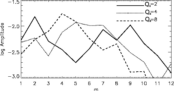
An important region in Fig. 3.11 is . There is a peak in amplitude at for . These are the edge modes described above. They were not seen in linear calculations because those calculations focused on finding vortex modes, which have corotation at or close to local vortensity minima. The loss of low vortex modes with increasing self-gravity observed in linear calculations, is replaced by the increasing prominence of global edge modes. Fig. 3.11 shows the amplitude becomes more significant with increasing self-gravity.
The simulation does display evidence of global disturbances hindering vortex evolution. This transition case is difficult to analyse since both vortices and spirals develop, as indicated by evolutionary snapshots of in Fig. 3.12. Fig. 3.11 shows the low and high modes have comparable amplitudes in . However, if only averaged over the region , then in the mode was found to be dominant, because this spiral mode is global whereas vortex mode disturbances are localised to the edge (). Increasing self-gravity further, eventually edge modes become dominant, this is seen in the case in Fig. 3.10.


3.4.5 Evolution and merging of self-gravitating vortices
Disc self-gravity also affects nonlinear interaction between vortices. Fig. 3.13 compares surface density perturbations for a range of at Since the vortices emerge at roughly , they have evolved for a similar time. Typical growth times for vortex modes are , so the vortices have evolved for about , well into the nonlinear regime.
The snapshot for shows a single vortex resulting from merging of the initial vortices. The vortex disturbance is largely confined to within a local scale-height of the gap edge. A single large vortex is the typical result for simulations with no self-gravity (e.g. de Val-Borro et al., 2007, , and in Chapter 2) , although the self-gravitating vortex here is thinner than the completely non-self-gravitating simulation (Fig. 3.8). The disc shows vortex merging taking place, as individual surface density maxima can still be identified within the large vortex behind the shock. For , a single vortex forms at .
Fig. 3.13 shows that increasing the disc mass delays vortex merging. For , 5 vortices remain and for and , 7 vortices remain. They have not merged into a single vortex as happened when . A 25% increase in disc mass as causes merging to be delayed by . This suggests that increased gravitational interaction between vortices opposes merging.
As is lowered the inter-vortex distance increases. When their azimuthal separation can be larger than the vortex itself. Also, vortices become less elongated and more localised being symptomatic of gravitational condensation. Trailing wakes from vortices become more prominent as the vortices more strongly perturb the disc via their self-gravity. In fact, the planetary wake becomes less identifiable among the vortex wakes. Notice vortex wakes are mostly identified with vortices upstream of the planetary wake, rather than just downstream. Vortex wakes appear to detach from the vortex after passing through the planetary shock. There is a sharp contrast in gap structure between the and cases. The single vortex that results when is aligned along the outer gap edge, which is still approximately identified as circle However, when the vortices and their wakes intersect the circle making the radius of the outer gap edge less well-defined.


An important feature of vortices is their wakes are associated with the excitation of density waves which transport angular momentum transport outwards (Paardekooper et al., 2010a, see e.g.), even without self-gravity. A measure of this can be made through the viscosity parameter. Here, it is defined as
| (3.40) |
where denote deviation from azimuthal averaged values. For diagnostics, is spatially averaged over the vortex region and its running-time average is plotted in Fig. 3.14. The parameter associated with vortices is , an order of magnitude larger than the imposed value associated with When , decays steadily after an initial transient growth. The case has a roughly constant for after a brief growth around . Interestingly, for intermediate strengths of self-gravity, —3.5, there is growth in over several tens of orbits.
The behaviour of as a function of is consistent with the general picture of vortex formation and evolution (Fig. 3.13). The decay in is associated with vortex merging leading to fewer vortices. This is the case for . Vortex merging happens more readily for lower disc masses, hence although multiple vortices develop from the instability, this phase does not last long enough for the multi-vortex configuration to significantly transport angular momentum. Increasing self-gravity to , vortices become less prone to merging and the multi-vortex phase lasts longer. They have time to evolve into compact objects that further perturb the disc. This is consistent with fact that -growth is prolonged with increased disc mass, as merging is delayed. However, if self-gravity is too strong, such as when , growth is again limited, because the global spiral mode develops and hinders vortex evolution.

3.4.6 Long term evolution of gap edge vortices
The long term evolution of vortices in the disc is shown in Fig. 3.15. It shows the instantaneous viscosity parameter, average over-density (defined in regions where the relative surface density perturbation is positive) and contour plots of relative surface density perturbation in the vortex region.
The viscosity parameter grows from to with , which is times larger than the background viscosity. At there remains 6 distinct vortices (one vortex just passing through the planetary wake). The multi-vortex configuration has been maintained for a further since Fig. 3.13. With weak self-gravity, a single vortex would have formed through merging. Delayed merging allows individual vortices to evolve and become planet-like. The typical over-density in a vortex is at and increases to by As a consequence one expects increased disturbance in the surrounding disc. The phase of -growth correlates with a linear increase in the average over-density in the vortex region.


At , Fig. 3.15 shows 6 vortices still remain, and the parameter is a maximum. However, after a burst of vortex merging events, decreases rapidly. The snapshot at shows a quieter disc with only 3 vortices, but of similar size to those before merging. This is unlike cases with weak self-gravity where a larger vortex results from merging. Fig. 3.16 compares post-merging vortices in discs with and For , the post-merging vortices are localised in azimuth, with and the contour plot shows the densest vortex has an over-density of . However, for the disc with , a single vortex forms that extends about half the total azimuth and has . This hints at gravitational collapse of vortices in the disc.
Note that the mass of the disc is only , usually considered insufficient for fragmentation into bound objects by classic Toomre instability (though it is still massive compared to more typical protoplanetary disc masses of ). However, the comparison above shows that adding self-gravity to the vortex instability enables collapse into compact objects that survive against shear.


Vortices in noticeably affect the gap structure. Fig. 3.17 shows several snapshots of the gap structure from when there were multiple vortices, to the end of the simulation when a vortex pair remained. The quasi-steady gap profile for is also shown for comparison. Neither the single vortex in nor multiple vortices with affect the one-dimensional gap profile at because the disturbances only redistribute mass in the azimuthal direction. However, in the disc, the original bump at the outer gap edge is diminished after vortex merging takes place at A surface density depression of then develops at and a bump develops at These features last to the end of the simulation.
Self-gravitating vortices behave like planets. Assuming vortices lie near the surface density maximum at the creation of the surface density deficit in and the new surface density maximum at could be induced, in a similar manner as it would be by a planet, through the outward transport of angular momentum by the density waves launched by the vortices.
Roughly speaking, treating vortices at as a gravitational perturbation on the exterior disc, it exerts a positive torque at . Inserting and (Fig. 3.15—3.16) gives . The material removed from the region of the deficit, which has gained angular momentum, ends up contributing to the new surface density maximum at

3.4.7 Anticyclonic vortices
For the disc, a vortex-pair forms at and lasts until the end of the simulation () and is reminiscent of co-orbital planets. The pair survives on a timescale well beyond which merging occurs in non-self-gravitating simulations. A snapshot is shown in Fig. 3.18(a). Two blobs can be identified along the gap edge, the upper vortex being more over-dense than the lower one. They lie at a radius , corresponding to local surface density maximum in azimuthally averaged one-dimensional profiles, which is expected to be neutral for vortex migration (Paardekooper et al., 2010a).
The upper vortex in Fig. 3.18(a) is different to the pre-merging vortices or those with weak self-gravity. It has two spiral disturbances extending from the vortex to , whereas the pre-merging vortices have one trailing spiral. Its vortensity field is shown in Fig. 3.18(b). The vortex core has , whereas the final large vortex in the disc with has in its core (though it is still a local minimum).
The region with has a mass of and average radius about the vortex centroid. It has semi-major and semi-minor axes of and respectively, corresponding to aspect-ratio of 2.9. This is about 18 Earth masses if is Solar. Denoting the mean square relative velocity (to the vortex centre) as , . This region is gravitationally bound. Although planets of such mass are not expected to open significant gaps, the surface density deficit in in Fig. 3.18(a) indicates vortices may do so. The process could be assisted by the fact that a vortex of size produces a perturbation of a magnitude similar what would be produced by Saturn when (Paardekooper et al., 2010a).
Finally, Fig. 3.18(c) show for a pair of Kida-like vortices placed in a disc. Note the similarity between the Kida-like vortex and the upper vortex in Fig. 3.18(a), particularly the double wake structure, the tilted core and the surface density deficit just outside the vortices. This is a surprising coincidence, given that the simulation setups that produced them were completely different (for more details see below).


3.5 Simulations of co-orbital Kida vortices
One of the effects of self-gravity shown in simulations above is to delay vortex merging. This effect is significant when vortices develop into compact structures. Furthermore, the similarity between the final vortex in the disc with and a Kida-like vortex (Kida, 1981) motivates one to consider the effect of self-gravity on the interaction between two Kida vortices.
Simulations presented here are supplementary and focus on the interaction between vortices without a planet. This isolates effects due to vortex-vortex interactions and the influence of self-gravity without interference from the planet.
3.5.1 Numerical setup
A standard power law disc is adopted, with initial surface density profile where is a scaling constant. The disc occupies . The value of is chosen to provide a specified at a specified radius as before. The initial azimuthal velocity is chosen so that the disc is initially in hydrostatic equilibrium. The initial radial velocity is zero. The disc is locally isothermal with . The viscosity is which is essentially the inviscid limit. No planets are introduced and the notation is used to denote a vortex centroid.
Artificial vortices are set up by following Lesur & Papaloizou (2009). Details of the implementation is described in Appendix 12. Two vortex perturbations are imposed with initial angular separation 33 3 Not to be confused with the polar angle in 3D.. Table 3.1 summarises the numerical experiments, which considers switching self-gravity on or off, a range of disc masses (here specified through ) and initial radial separations of the two vortices (so that for one of the vortices, ).
The fluid equations are evolved using the FARGO code with resolution giving grid points per scale height. The vortices are typically of that size. Damping boundary conditions are applied (de Val-Borro, 2006).
| Case | self-gravity | ||
|---|---|---|---|
| Fnsg | 0 | 8.0 | NO |
| Fsg | 0 | 8.0 | YES |
| M1 | 0 | 15.9 | YES |
| M2 | 0 | 5.3 | YES |
| S1 | 0.1 | 8.0 | YES |
| S2 | 0.2 | 8.0 | YES |
| S3 | 0.3 | 8.0 | YES |
| S4 | 0.6 | 8.0 | YES |
3.5.2 Vortex pairs
As an example of vortices formed by the above procedure, Fig. 3.19 shows the vortensity field for the case Fnsg. The vortex pair circulates at and are localised in radius and azimuth. The vortex centroids have vorticity (dimensionless units) in the non-rotating frame, close to the local Keplerian shear (). The upper vortex has a long tail reaching the outer part of the lower vortex rather than its centroid. The wakes associated with each vortex are similar to those induced by a planet and is responsible for vortex migration (Paardekooper et al., 2010a).
Focusing on one vortex, the region with negative absolute vorticity has half width in radius and azimuth of and respectively.This region has mass , or about if . The estimate is not far from the assumption that the final vortex has size with average density that of the unperturbed disc at the location it was set up, which gives . If self-gravity is enabled, one can expect gravitational interaction between vortices to behave like that between two co-orbital planets of at least a few Earth masses.

3.5.3 Simulation results
Consider first the cases Fsg and Fnsg. These are for the disc with with and without self-gravity respectively. The distance between vortex centroids as a function of time is shown in Fig. 3.21(a). It takes almost 5 times as long for the self-gravitating vortices to merge. A merging event is shown in Fig. 3.20.
By examining the vortensity distribution, non-self-gravitating vortices were observed to begin merging at but self-gravitating vortices at For Fnsg, vortices approach each other within of formation and merge. Assuming they move relative to each other because of Keplerian shear, the time taken to merge implies that their radial separation at vortex formation must be This length-scale is only resolved by about 2.5 grid cells indicating that a non-zero initial separation is generated by grid effects, despite the vortex perturbations being imposed at the same radius. This is actually not unphysical because vortex formation through instability is not expected to occur at exactly the same radii.


In the self-gravitating case Fsg, the inter-vortex distance oscillates with period and there are two close-encounters before merging. This is analogous to the survival of the vortex pair towards the end of the disc-planet simulation for . Given a maximal separation of and that the vortices are circulating near unit radius, the maximal angular separation is . The minimal separation during the first two close encounters is , or about which implies that the vortices are on tadpole orbits. As the minimum separation is much larger than the typical vortex size, merging does not occur during the first two close encounters.
The experiment in Fig. 3.21(b) varies the strength of self-gravity via . The reference case has . Doubling to (case M1) weakens self-gravity and vortices merge within few tens of For (case M2) the oscillation period is and maximal separation is 1.55, larger than for , as is the first minimum separation: the increased self-gravity has enhanced the mutual repulsion of vortices. The two-vortex configuration in M2 lasts until the end of the simulation, but there is a secular decrease in the minimum separation (of at and at ) due to vortex migration. Merging will likely occur eventually. Consistent with the behaviour seen for gap edge vortices, increasing self-gravity delays merging.
The final experiment varies the initial radial separation of the vortex perturbations. Results are shown in Fig. 3.21(c). Increasing to from the reference case, the first minimum separation decreases to 0.45 from 0.6: vortices approach each other more closely, but still repel and undergo co-orbital dynamics. The increased oscillation amplitudes imply a larger tadpole orbit. For and , vortex separation decreases more rapidly and become small enough for vortex merging. However, for , vortices simply circulate past by each other and no merging occurs, despite reaching a similar minimal separation as when . Vortices should collide head on if they are to merge.


3.5.4 Vortices as co-orbital planets
Simulations above indicate that self-gravitating vortex pairs behave like co-orbital planets. This means there exists an initial radial separation (or impact parameter) below which vortices execute horseshoe orbits relative to each other. Analytical and numerical work indicates that vortices merge if their centroids are within of each other (Zabusky et al., 1979; Melander et al., 1988, e.g.), where is the vortex size. Although one cannot assume the same critical apply here because the situations are very different, it is still reasonable to expect merging if vortices can reach within some critical distance of one another.
The results above can be anticipated from existing treatments of co-orbital dynamics. The first is Murray & Dermott (2000)’s model of the co-orbital satellites of Saturn, the Janus-Epimetheus system. The governing equation from Murray & Dermott (2000) gives a relationship between two configurations, the ‘final’ configuration (subscript ) and the ‘initial’ configuration (subscript ) in the form
| (3.41) | ||||
where is the radial separation of the satellites, the average orbital radius (assumed fixed, thereby ignoring migration), their angular separation and with being the sum of the satellite masses. It is assumed
Eq. 3.41 should apply to vortex pairs if there is significant mutual gravitational interaction. Their final radial separation is assumed zero, , when the vortices are at their minimum angular separation. Inserting (corresponding to the initial conditions deduced for Fnsg), and (corresponding to the measured mass of the negative absolute vorticity region in Fsg), Eq. 3.41 gives or a minimal angular separation of so merging is not expected if vortices have size This estimate is lower than the observed value of 0.6, but this is a lower limit on the vortex mass. Inserting gives assuming all other parameters remain the same. This implies the effective gravitational mass of the vortex should be 20 Earth masses.
Eq. 3.41 is illustrated in Fig. 3.22. For fixed and increasing (e.g. as a by product of increasing the disc mass) the minimal separation increases, eventually becoming too large for merging to occur. For fixed decreases as increases. This is similar to a test particle on a horseshoe orbit in the restricted three body problem. The larger its impact parameter, the closer it approaches the secondary mass.

Mutual horseshoe turns may also be analysed in a shearing sheet approximation. This is just the generalisation of the result for a test particle and a planet, to the two-planet case (Appendix 8.A). Since the vortices have characteristic sizes of the local scale-height, it is convenient to non-dimensionalise lengths by , in the expression for the maximum initial radial separation of vortices that allow horseshoe turns:
| (3.42) |
where . Given , Eq. 3.42 can be inverted to give the range of possible This inequality is displayed in Fig. 3.23. There exists a critical beyond which vortices do not execute horseshoe turns and instead circulate past each other. There may also exist a value such that and for , vortices execute U-turns and the values of attained are sufficiently small to allow merging. This happens only when the vortices have small enough mass. When , can be larger than critical, so that merging does not occur.

These simple models give qualitatively the same results as vortex pair and disc-planet simulations, and serve to explain the effect of self-gravity delaying merging by interpreting vortices as co-orbital planets that execute mutual horseshoe turns, thereby imposing a minimum inter-vortex separation (mainly in the azimuthal direction). If this minimum separation is still larger than a critical separation known to exist for vortex merging, then merging cannot occur. Hence, multiple-vortex configurations can be sustained longer as the strength of self-gravity is increased.
3.6 Implications on vortex-induced migration
Chapter 2 established that vortices at gap edges can lead to brief phases of rapid inwards migration of giant planets. In summary, gap edges become unstable to vortex modes leading to vortex mergers on dynamical timescales, in turn resulting in a large-scale vortex circulating at either gap edge. Upon approaching the planet, the inner vortex can execute a horseshoe turn and move outwards across the gap, gaining angular momentum. Thus, the planet loses angular momentum and is scattered inwards.
For comparison purposes, the non-self-gravitating simulations performed in Chapter 2 were repeated with disc self-gravity. Fig. 3.24 shows the orbital migration of a Saturn-mass planet in discs with total mass and . For , the surface density perturbations are also compared in Fig. 3.25. The non-self-gravitating disc was the fiducial run in Chapter 2. Including self-gravity delays vortex-induced migration from to The delay is consistent with both the stabilisation of low modes, and the slower vortex merging induced by self-gravity.


Consider . In the self-gravitating disc, it takes longer for the inner vortex to build up (e.g. comparing in Fig. 3.25), disrupt the coorbital region and flow across the gap. This delays vortex-induced rapid migration, by about compared to the non-self-gravitating case.
The extent of rapid migration is unaffected by self-gravity. Notice also the increased oscillations in when self-gravity is included. This is because of the sustained multi-vortex configuration at the outer gap edge causing large oscillations in disc-planet torques, whereas without self-gravity these vortices would have merged.
After the first scattering event, migration stalls while the planet opens a gap at its new orbital radius and vortex formation recurs. With self-gravity included, the re-formation of a single vortex takes longer and it is narrower in radial extent than the non self-gravitating case. When the thinner self-gravitating vortex passes by the planet, little vortex material splits off from the main vortex and flows across the gap, unlike the non-self-gravitating vortex where material breaks off more easily (Chapter 2). This is probably due to the self-gravity of the vortex. Hence, there is a longer stalling period when self-gravity is included. Thus the net effect of self-gravity is to slow the migration in this example.
For the setup used in Chapter 2, a second fast migration episode was not seen within the simulated time when self-gravity was included, but it may eventually occur. The total practical simulation time of a few hundred orbits is still very short compared to disc lifetimes. However, for the disc model used in previous parts of this Chapter, two episodes of rapid migration occurs (Fig. 3.26). Self-gravity does not change the physical nature of vortex-induced, non-smooth migration.

3.7 Summary and discussion
The effect of disc self-gravity on vortex-forming instabilities associated with planetary gaps were explored. Analysis shows vortex modes are stabilised by self-gravity through its effect on the linear mode when the background remains fixed. This aspect has been confirmed by linear calculations. Linear calculations showed that the vortex forming modes with the highest growth rate shift to higher with increasing disc mass. This is due to the combined effect of self-gravity through the response and through the background state.
Hydrodynamic simulations with and without self-gravity for a range of disc masses were performed. More vortices form as the disc mass increased in accordance with linear calculations. However, for sufficiently strong self-gravity, the vortex modes are suppressed and global spiral modes develop instead. Self-gravity delays vortex merging and multi-vortex configurations can be sustained for longer with increasing disc mass, allowing vortices to evolve individually.
The nature of post-merging vortices is also affected by self-gravity. With weak self-gravity ( i.e. ), a single vortex, extended in azimuth forms and circulates at the outer gap edge. For the final configuration is a vortex pair at the outer gap edge, each localised in azimuth. In this case a vortex, containing on the order of , is gravitationally bound. The effect of their gravitational influence on the rest of the disc is to redistribute mass radially whereas for lower disc masses, redistribution is restricted to being azimuthal.
The internal flow in these self-gravitating, localised vortices adjusts so that they are not destroyed by the background shear, taking on a structure similar to that of a vortex resulting from perturbing the disc with the Kida solution (Kida, 1981). Such vortices form in discs much less massive than that required for direct disc fragmentation. Vortices can trap dust particles due to their association with pressure maxima (Bracco et al., 1999; Chavanis, 2000). Increasing self-gravity leads to vortices of stronger density contrast (Fig. 3.16), so self-gravitating vortices may be more effective at collecting solid particles, and assist planetesimal formation.
Supplementary simulations of Kida-like vortices were performed to understand the effect of self-gravity on inter-vortex interactions. In a self-gravitating disc, coorbital vortex pairs behave like coorbital planets and can execute mutual horseshoe turns. As a consequence there exists a minimum inter-vortex distance. Merging is then avoided if this minimal separation is still larger than a critical separation below which vortex merging occurs.
The effect of self-gravity found here, should also applicable to other types of structured features in a protoplanetary disc that could support vortex forming instabilities. Such a possibility is the boundary region between a dead zone and active region of the disc (Lyra et al., 2009).
The basics of vortex-induced migration remains unchanged by self-gravity. With self-gravity, the resistance to forming a single large vortex results in such migration being delayed. Self-gravitating vortices are are less effective in scattering the planet because they do not disrupt the co-orbital region as significantly as their non-self-gravitating counterparts. It can be said that in the regime of disc masses where vortices form and are significantly affected by self-gravity, vortex-induced migration is slowed down.
Chapter 4 Edge modes in self-gravitating discs
Numerical experiments Chapter 3 showed that global spiral disturbances associated with gap edges can develop in massive discs. They arise from a linear instability associated with both the self-gravity of the disc and local vortensity maxima which coincide with gap edges. They can be physically interpreted as disturbances localised around a vortensity maximum that further perturb gravitationally the smooth parts of the disc by exciting waves at Lindblad resonances. The angular momentum carried away reacts back on the edge disturbance so as to destabilise it.
These edge modes are studied in this Chapter. The disc-planet models are identical to that used in Chapter 3, but briefly reproduced in §4.1 for ease of reference. In §4.2, the existence of edge modes and its basic features are illustrated with a numerical simulation. An analytic discussion and interpretation of edge modes is then presented in §4.3—§4.4. In §4.5, linear calculations for various disc models confirm the existence of edge dominated modes for low values of the azimuthal mode number. The physical picture of edge modes presented in the analytical discussion is consistent with these numerical solutions.
In §4.6 results from hydrodynamic simulations for a range of disc masses are discussed. These are all stable in the absence of the planet. However, they exhibit low edge modes once a planet-induced gap is present. The form and behaviour of these is found to be in accord with linear theory. The spiral arms associated with the edge instabilities are shown to produce fluctuating torques acting on the planet. Fast inwards type III migration may occur, but outwards migration due to interaction with spiral arms is also observed. §4.8 concludes this Chapter.
4.1 Disc model
To apply angular momentum conservation in the analytical description of edge modes, three-dimensional disc models are required. This is because although the disc material may be considered to be confined to a thin sheet, the gravitational potential it generates is still three-dimensional. Thus, it is important to consider the self-gravity part as fully three-dimensional. This is governed by the Poisson equation
where is the three dimensional mass density and is the associated gravitational potential which can be found via
| (4.1) |
where is the domain where is non zero. This coincides with the disc domain when this is not separated from external material. The full 3D hydrodynamic equations are listed in §1.4 and is the basis for analytical work. In analytic discussions, fluids with a general barotropic equation of state are considered, for which and
4.1.1 Razor thin discs
For numerical work, the disc is considered two-dimensional and only its gravitational potential in the plane is used. The governing equations are therefore those listed in §1.4.6, which were used throughout Chapter 3. In numerical experiments, the locally isothermal equation of state is used with fixed aspect-ratio . The physical setup and notation is the same as Chapter 3, but simulations will be presented for a range of viscosity and softening parameters.
The discs occupy and are parametrised by , the Keplerian Toomre value at the outer boundary. The initial surface density profile is given by Eq. 3.1 (Chapter 3). Recall that 2D self-gravity requires the use of a gravitational softening length (see §1.4.6, Eq. 1.21) to prevent a singularity and approximately account for the vertical dimension. The softening length prescription is used, and set as a fiducial value, but values up to 1.0 will be considered.
The initial azimuthal velocity is found by assuming the centrifugal force balances forces due to stellar gravity, the disc’s self-gravity and pressure gradient. Thus the initial azimuthal velocity is given by
| (4.2) |
For the local isothermal equation of state adopted, the contribution due to the pressure is given by
| (4.3) |
At for this is which is approximately of the square of the local Keplerian speed so that the contribution of the pressure force is indeed minor when compared to that arising from the gravity of the central star.
The initial radial velocity is set to , corresponding to the initial radial velocity velocity of an one-dimensional Keplerian accretion disc with and uniform kinematic viscosity. The fiducial value in dimensionless units is adopted, but results for to will be presented. The disc is evolved for Keplerian orbits at before introducing the planet.
When a planet of mass is introduced, it is inserted in a circular orbit, under the gravity of both the central star and disc, at a distance from the central star. Its gravitational potential is then ramped up over a time interval Recall is the circular Keplerian orbital period at the planet’s initial radius.
4.2 Properties of edge modes
The existence of spiral modes associated with planetary gaps is first demonstrated through numerical simulations. Numerical details are given in §4.6 where additional hydrodynamic simulations of this type as well as others, where the planet is allowed to migrate, will be investigated more fully.
4.2.1 Example simulation
Described here are results obtained for the disc model, corresponding to a total disc mass of , in which there is an embedded planet with mass The uniform kinematic viscosity was taken to be in dimensionless units. For this simulation the planet was held on a fixed circular orbit. Without a perturber the disc is gravitationally stable because the near the planet and the outer boundary, respectively. General non-axisymmetric gravitational instabilities occur in smooth discs when .
The profile of the gap opened by the planet is shown in Fig. 4.1 in terms of the azimuthally averaged surface density , vortensity and Toomre . The latter is calculated using the azimuthally averaged epicycle frequency. The surface density gap corresponds to a decrease of surface density by relative to the initial profile.
Notice that the vortensity and Toomre profiles are qualitatively similar. The neighbourhoods of the inner and outer gap edges both contain maxima and minima of and For typical disc models structured by disc-planet interactions, such as those illustrated in Fig. 4.1, local maxima/minima in and approximately coincide. Vortensity generation as material flows through planet-induced shocks leads to vortensity maxima. Since the axisymmetric Toomre parameter can be directly related to vortensity, , the resulting and profiles are very similar in their extrema locations.
Fig. 4.1 shows that in the neighbourhood of the outer gap edge, the maximum and minimum values of occur at and and are and respectively. In the region of the inner gap edge, the maximum and minimum values of occur at and These are and respectively. The characteristic width of the gap edge is the local scale-height. On average for . Since everywhere, the disc is stable against local axisymmetric perturbations. Furthermore, since in the gap region, gravitational instabilities should not be directly associated with the local value of . Instead, instability is associated with the global -profile.

The simulation shows that both gap edges become unstable. The surface density contours at are shown in Fig. 4.2. A mode with azimuthal wavenumber and relative surface density perturbation is associated with the inner edge and a mode with and associated with the outer edge. The modes have become nonlinear, with the development of shocks, on dynamical time-scales. Spirals do not extend across the gap indicating effective gap opening by the planet and disc self-gravity is not strong enough to connect the spiral modes on either side of

Plots of the radial dependence of the pattern rotation speed 11 1 The pattern speed is , where . Recall is the Fourier amplitude. Calculating the pattern speed thus require . However, from the continuity equation. Instantaneous time-derivatives can therefore be calculated from spatial derivatives. This gives the pattern speed from a single data output., obtained from the component of the Fourier transform of the surface density, together with the azimuthally averaged values of and are presented in Fig. 4.3. The mode associated with the outer gap edge is of particular interest, because the spiral mode has more than twice the relative surface density amplitude compared to the inner spiral mode.
By necessity, the Fourier transform includes features due to the planetary wakes and inner disc spiral modes as well as the dominant outer disc mode. On average, . This value was also explicitly checked by measuring the angle through which the spiral pattern rotates in a given time interval. There is a co-rotation point in the outer disc at where , i.e. at the local vortensity maximum (surface density minimum) of the basic state, which is just within the gap (see Fig. 4.1). This is consistent with pattern speeds obtained from linear calculations presented later. Fig. 4.3 indicates another co-rotation point at but this is due to inclusion of features associated with the planetary wakes.

Unstable spiral modes identified here are referred to as edge modes. Their properties can be compared to those of groove modes in particle discs (Sellwood & Kahn, 1991) or fluid discs (Meschiari & Laughlin, 2008). Sellwood & Kahn describe groove modes as gravitational instabilities associated with the coupling of disturbances associated with two edges across the gap between them. However, the analytic description of the edge mode instability, presented later, is a coupling between a disturbance at a single gap edge and the disturbance it excites in the adjoining smooth disc away from co-rotation. The other gap edge plays no role in this description. Although both types of mode are associated with vortensity maxima, the groove modes described above would have co-rotation at the gap centre midway between the edges, whereas for the planetary gap co-rotation is at the gap edge.
This is significant because it implies differential rotation between the spiral pattern and the planet. In addition, unstable modes on the inner and outer gap edges need not have the same (Fig. 4.2 shows on the inner edge and on the outer edge). If there was a groove mode with co-rotation at the gap centre, then the spiral pattern would co-rotate with the planet and the coupled edges must have disturbances dominated by the same value of .
4.2.2 Comparison to vortex instabilities
It is interesting to compare edge modes to the localised vortex-forming instabilities studied in Chapter 2—3, which develop in non-self-gravitating or weakly self-gravitating discs near gap edges. However, the vortex instability requires low viscosity. For comparison purposes, here a kinematic viscosity of is imposed. The behaviour of disc models with and are compared below, the former having strong self-gravity and the latter weak self-gravity.
Fig. 4.4 shows two types of instabilities depending on disc mass. The lower mass disc with develops 6 vortices localised in the vicinity of the outer gap edge. The more massive disc with develops edge modes of the type identified in the earlier run with Here, the spiral mode is favoured because of the smaller viscosity coefficient used 22 2 This results in a sharper gap profile, which generally supports higher .
Vortex modes are said to be local because instability is associated with flow in the vicinity of co-rotation (Lovelace et al., 1999) and does not require the excitation of waves. Edge modes are said to be global because instability requires interaction between an edge disturbance and waves launched at Lindblad resonances, away from co-rotation in the smooth part of the disc. Vortices perturb the disc even without self-gravity (Paardekooper et al., 2010a). Although the vortex mode in Fig. 4.4 shows significant wave perturbations in the outer parts of the disc, these should be seen as a consequence of unstable vortices forming around co-rotation, rather than the cause of a linear instability.
Vortex modes have co-rotation close to local vortensity minima in the undisturbed gap profile. The self-gravitating vortex modes are localised with higher being dominant (). On the other hand the spiral modes found here are global with . Edge modes make the gap less identifiable than vortex modes do because the former, with corotation closer to , protrudes the gap edge more. While the edge mode only takes a few to become non-linear with spiral shocks attaining comparable amplitudes to the planetary wakes, the vortex mode takes a significantly longer time (the plot for is after gap formation). This can be understood as waves emitted by the vortex modes tends to stabilise them, whereas wave emission drives the edge mode instability.


4.3 Analytical discussion of edge modes
The fiducial disc simulated above is massive with but it is still stable against gravitational instabilities in the sense that everywhere and the disc without an embedded planet, which has a smoothly varying surface density profile, does not exhibit the spontaneous growth of spiral instabilities. A planet of Saturn’s mass () is expected to only open a partial gap ( deficit in surface density), but even this is sufficient to trigger a spiral instability.
The case above thus suggests spiral modes may develop under conditions that are not as extreme as those considered by Meschiari & Laughlin (2008). They used a prescribed gap profile with a gap depth of relative to the background, which is three times deeper than the simulation above. Their gap corresponds to , although a planet potential was not explicitly included. In both their model and the fiducial case, the gap width is , but since Meschiari & Laughlin effectively used a two Jupiter mass planet, at the same their gap is about 1.9 times wider than for a Saturn mass planet.
This section and the next are devoted to a theoretical discussion of spiral modes associated with planetary gap edges. This work is based on the analysis of the governing equations for linear perturbations. As angular momentum balance is important for enabling small perturbations to grow unstably, one begins by formulating the conservation of angular momentum for linear perturbations.
4.3.1 The conservation of angular momentum for a perturbed disc
A conservation law can be derived for angular momentum associated with the perturbations of a disc. This enables the angular momentum density and flux to be identified within the framework of linear perturbation theory. The behaviour of these quantities is found to be important for indicating the nature of the angular momentum balance in a system with a neutral or weakly growing normal mode and how positive (negative) angular momentum fluxes associated with wave losses may drive the instability of a disturbance that decreases (increases) the local angular momentum density.
4.3.2 Barotropic discs
The linearised equation of motion in three dimensions for the Lagrangian displacement for a differentially rotating fluid with a barotropic equation of state and with self-gravity included is given by
| (4.4) |
where
| (4.5) |
(Lynden-Bell & Ostriker, 1967; Lin et al., 1993, see eg.). A cylindrical polar coordinate system is adopted here. Perturbations to quantities are denoted with . The operator is the convective derivative following the unperturbed motion and is the unit vector in the direction which is normal to the disc mid-plane. For perturbations that depend on through a factor being the azimuthal mode number, assumed positive, the operator reduces to the operator In addition, for a barotropic equation of state, depends only on the cylindrical radius. Then Eq. 4.4 becomes
| (4.6) |
The Eulerian density perturbation is given by
| (4.7) |
The perturbation to the disc’s gravitational potential is given by linearising Poisson’s equation to give
| (4.8) |
An external potential perturbation has been added to the equations of motion to assist with the identification of angular momentum flux later on.
By taking the scalar product of Eq. 4.6 with and taking the imaginary part, after making use of Eq. 4.7 and Eq. 4.8, a conservation law that expresses the conservation of angular momentum for the perturbations can be derived:
| (4.9) |
where
| (4.10) | ||||
| (4.11) | ||||
| (4.12) | ||||
| (4.13) |
and
| (4.14) |
Here is the angular momentum density and the angular momentum flux is split into three contributions, being proportional to the Lagrangian displacement, is the advective angular momentum flux, is the flux associated with the perturbed gravitational stresses and is the flux associated with the external potential which is inactive for free perturbations.
The quantity is a torque density associated with the external potential as can be seen from that fact that the real torque integrated over azimuth and divided by is
| (4.15) |
The dependence has been reinstated on the LHS for clarity. This justifies the scalings used for the angular momentum density and fluxes.
4.3.3 Two dimensional discs
The form of the conservation law for a razor thin disc is obtained by integrating Eq. 4.9 over the vertical coordinate. For terms the integrand is non zero only within the disc. may be assumed to depend only on and The effect of the integration is simply to replace and by the surface density and its perturbation respectively. The fluxes become vertically integrated fluxes. Vertically integrating the term associated with the gravitational stresses, assuming the potential perturbation vanishes at large distances, gives
| (4.16) |
where has been used. The angular momentum flux associated with self-gravity is
| (4.17) |
Thus for a two dimensional razor thin disc the conservation law is of the same form as Eq. 4.9 but with , and given by Eq. 4.10, Eq. 4.11 and Eq. 4.13 with replaced by respectively. As the vertical direction has been integrated over only the radial components of the fluxes contribute. From the above analysis the vertically integrated angular momentum flux due to gravitational stresses becomes
| (4.18) |
with given by Eq. 4.17. Accordingly this term, unlike the others involves an integration over the vertical direction. Explicit expressions for the fluxes in terms of the perturbation , appropriate to the razor thin disc, shall be derived below.
4.3.4 Locally isothermal equation of state
It is possible to repeat the analysis of §4.3.1 when the disc has a locally isothermal equation of state. In this case where is a prescribed function of position and the linearised equation of motion (Eq. 4.4) is modified to read
| (4.19) |
An expression of the form of Eq. 4.9 may be derived but now the torque density takes the form
| (4.20) |
When is constant corresponding to a strictly isothermal equation of state, the fluid is again barotropic and previous expressions recovered. Eq. 4.20 contains terms in addition to external contributions. In general these imply the possibility of an exchange of angular momentum between perturbations and the background. A very similar discussion applies to the razor thin limit. The analysis above can be applied to determine the angular momentum balance for the linear perturbations of razor thin discs and thus determine properties of and conditions for unstable normal modes.
4.3.5 Properties of the linear modes of a razor thin disc
Linear perturbations are assumed to have and dependence through a factor of the form where is the complex eigenfrequency and is the azimuthal mode-number. From now on this factor is taken as read. Linearising the hydrodynamic equations for the inviscid case and ignoring external potentials, gives
| (4.21) | ||||
| (4.22) | ||||
| (4.23) |
Recall is the shifted mode frequency. These equations were also used in Chapter 2 and Chapter 3 in terms of . However, it is convenient for the analytical discussion later on, to derive a governing equation in a slightly different form than previous Chapters. Using Eq. 4.22 and Eq. 4.23 to eliminate and in Eq. 4.21 gives
| (4.24) |
Recall and . This form is similar to that used by Papaloizou & Savonije (1991) and explicitly shows that a co-rotation singularity, where , can be avoided if co-rotation corresponds to a vortensity extremum (). The potential singularity at co-rotation associated with the term involving has negligible effect in practice, explained below.
The above expressions may be applied to a disc, either with a locally isothermal equation of state, or with a barotropic equation of state, where the integrated pressure and the sound-speed . To obtain the latter case , the quantity is simply replaced by zero. Inclusion of additional terms dependent on this has been found numerically to produce only a slight modification of the discussion that applies when they are neglected. This is because the locally isothermal varies slowly compared to either the linear perturbations or the surface density in the vicinity of an edge, thus shall be neglected in the analysis from now on. Also recall that and the gravitational potential is given by the vertically integrated Poisson integral as
where
Here the domain of integration is that of the disc provided there is no external material. However, in a situation where density waves propagate beyond the disc boundaries either should be formally extended or the form of changed to properly reflect the boundary conditions.
The governing equation above, together with angular momentum conservation, can be used to model angular momentum flux balance for normal modes. For simplicity only barotropic case are considered in the analysis. The analytic discussion concerns a disc model with one boundary being a sharp edge with arbitrary propagation of density waves directed away from this boundary being allowed. When applied to a gap opened by a planet in a global disc, the analytic models corresponds to the section of the disc from the inner disc boundary to the inner gap edge or the section from the outer gap edge to the outer disc boundary. These two sections are assumed to be decoupled in the analytic discussion of stability but not in the numerical one. In addition, although it produces the background profile, the planet is assumed to have no effect on the linear stability analysis discussed here, but it is fully incorporated in nonlinear simulations. The correspondence between the various approaches adopted indicates the above approximations are reasonable. The discussion of the outer and inner disc sections is very similar, accordingly these are considered below together.
4.3.6 Angular momentum flux balance for normal modes
The vertically integrated angular momentum flux associated with perturbations can be related to the background vortensity profile. A barotropic disc model is assumed, so terms involving are neglected. Multiplying Eq. 4.24 by and integrating:
| (4.25) |
where, here and below, the positive sign alternative applies to the case where the disc domain has an inner sharp edge where and then the outer boundary radius. The negative sign alternative applies to the case where the disc domain has an outer sharp edge where and then the inner boundary radius. In both cases waves may propagate through Note also that there is no contribution from edge boundary terms as the surface density is assumed to be negligible there.
One may now express the terms in the above integral relation, which for convenience has been taken to define a functional of that depends on in terms of quantities related to the transport of angular momentum by taking its imaginary part. One begins by assuming is real or, more precisely, the limit that marginal stability is approached.
By making use of Eq. 4.16, one finds that
| (4.26) |
Recall that is the vertically integrated angular momentum flux transported by gravitational stresses. Note that at the sharp edge is ignored. Eq. 4.16, together with the requirement that is regular for and vanishes more rapidly than for , implies that is zero at the sharp edge separating the disc domain and the exterior (assumed) vacuum or very low density region.
In addition, from Eq. 4.22 and Eq. 4.23, the radial Lagrangian displacement is given by
| (4.27) |
From this it follows that the imaginary part of the second term on the RHS of Eq. 4.25) is
Using the above and taking the imaginary part of Eq. 4.25 yields the remarkably simple expression
| (4.28) |
In the above, it has been assumed that is real and that the mode is at marginal stability. Then the RHS of Eq. 4.28 is apparently real. However, the integrand is potentially singular at corotation where Thus the approach to marginal stability has to be taken with care.
Setting where being the real part of defines the corotation radius, through and is the imaginary part of , so that the mode is unstable for with growth rate . Marginal stability can be approached by assuming that has a vanishingly small magnitude but is negative. Then one can apply the Landau prescription and replace by where indicates that the principal value of the integral is to be taken and denotes Dirac’s delta function. Adopting this, Eq. 4.28 becomes
| (4.29) |
The above relation can be viewed as stating that at marginal stability, either corotation is at a vortensity extremum and both terms in Eq. 4.29 vanish, or angular momentum losses as a result of waves passing through (the smooth boundary), are balanced by torques exerted at corotation. The latter torque is proportional to the gradient of the vortensity (Goldreich & Tremaine, 1979). Note that scales with .
The propagating waves quite generally carry negative angular momentum when located in an inner disc () and positive angular momentum when located in an outer disc () (Goldreich & Tremaine, 1979). Thus a balance may be possible between angular momentum losses resulting from the propagation of these waves out of the system and angular momentum gained or lost by an edge disturbance (near co-rotation radius) as expressed by Eq. 4.29. For an edge disturbance in a region of increasing (decreasing) surface density, such as an inner (outer) edge to an outer (inner) disc, the edge disturbance loses (gains) angular momentum.
In practice, an inner (outer) edge disturbance may be associated with a positive (negative) surface density slope near a vortensity maximum or near a vortensity minimum occurring as a result of the variation of both and (Lovelace et al., 1999; Papaloizou & Lin, 1989, e.g.). The former case is associated with discs for which self-gravity is important and spiral density waves are readily excited. The latter is associated with weakly or non self-gravitating discs and is associated with vortex formation at gap edges as has already been discussed in Chapters 2—3.
The boundary condition at (the non-sharp boundary) may correspond to stipulating outgoing waves or a radiation condition, so that the fluxes in Eq. 4.29 are non zero. Another possibility is to have a surface density taper to zero which would mean wave reflection and removal of the boundary flux terms. In fact, the issue of stability, for the particular modes of interest, is not sensitive to precise boundary conditions at the smooth boundary. In the case of non self-gravitating discs and the low vortex modes, the regions away from the edge are evanescent and amplitudes are small there, the disturbance being localised in the vicinity of the edge. For self-gravitating discs, as indicated below, instability can appear because of an unstable interaction between outwardly propagating positive (inwardly propagating negative) angular momentum density waves and a negative (positive) angular momentum edge disturbance localised near an inner (outer) disc gap edge. As long as these waves are excited it should not matter whether they are reflected or transmitted at large distance, as long as their angular momentum density remains in the wider disc and is not fed back to the exciting edge disturbance.
For these reasons and also simplicity it shall be assumed that at the boundary where either the surface density has tapered to zero, or there is reflection such that the boundary terms in expressions like Eq. 4.25 may be dropped. Eq. 4.29 then simply states that marginal stability occurs when corotation is at a vortensity extremum. It is found that the vortensity maximum case is associated with an instability in self-gravitating discs that is associated with strong spiral waves. On the other hand the vortensity minimum case is associated with the vortex-forming instability in non-self gravitating discs that has been previously studied.
4.4 Description of the edge mode instability
The edge mode instability in a self-gravitating disc can be interpreted as due to a disturbance associated with the edge causing the excitation of spiral waves that propagate away from it resulting in destabilisation. This occurs because the emitted waves carry away angular momentum which has the opposite sign to that associated with the edge disturbance ( see §4.3.6 and Eq. 4.29). Accordingly the excitation process is expected to lead to the growth of this disturbance.
Thus one can consider a disturbance localised in the vicinity of the edge and the potential perturbation it produces to excite spiral density waves in the bulk of the disc. Numerical calculations show that edge dominated modes of this type occur for low and are dominant in the nonlinear regime. The analysis below assumes the mode is weakly growing corresponding to the back reaction of the waves on the edge disturbance being weak. Thus in the first instance one calculates a neutral edge disturbance (zero growth rate) and then calculate the wave emission as a perturbation. It should be emphasised again that an important feature is that corotation is at a vortensity maximum (in contrast to the non-self-gravitating case for which corotation is located at a vortensity minimum). Such modes require self-gravity. In an average sense they require a sufficiently small value and so cannot occur in the non self-gravitating limit ().
4.4.1 Neutral edge disturbances with corotation at a vortensity maximum
Consider the expression for expressed by Eq. 4.24 and assume that only the vortensity gradient term (third term on the RHS) need be retained. This is because this term should dominate near corotation in the presence of large vortensity gradients that are presumed to occur near the edge and the disturbance is assumed localised there 33 3 See also the discussion of groove modes in collisionless particle discs of Sellwood & Kahn (1991), where similar assumptions are made.. Thus
| (4.30) |
where . The associated gravitational potential is given by
| (4.31) |
The relation gives the integral equation
| (4.32) |
For a disturbance dominated by self-gravity, pressure should be negligible. Under such an approximation, Eq. 4.30 then implies in order to obtain a negative (positive) potential perturbation for a positive (negative) surface density perturbation. At co-rotation where and there is a vortensity extremum, this requirement becomes . Since typical rotation profiles have , the physical requirement that potential and surface density perturbations have opposite signs implies that at co-rotation, i.e. the vortensity is a maximum. The discussion thus applies to vortensity maxima only. For the class of vortensity profiles for which the integral Eq. 4.32 may be transformed into a Fredholm integral equation with symmetric kernel. This is demonstrated below.
Noting that corotation is located at a vortensity maximum, the requirement above implies the vortensity increases (decreases) interior (exterior) to corotation 44 4 The discussion may also be extended to the case when that is true with vanishing at corotation. As the disturbance is expected to be localised around corotation, it is reasonable to assume this holds and that one may contract the integration domain to exclude regions which do not conform without significantly affecting the problem.
Next, introduce the function such that
| (4.33) |
where
| (4.34) |
Note that for , is real. Defining the new symmetric kernel as
| (4.35) |
where
| (4.36) |
one obtains the integral equation
| (4.37) |
In other words, is required to be the solution to
| (4.38) |
with . However, Eq. 4.38 is just a standard homogeneous Fredholm integral equation of the second kind. Thus the existence of a nontrivial solution () implies is an eigenfunction of the kernel with unit eigenvalue.
The kernel is positive and symmetric. Accordingly the Fredholm equation above has the property that the maximum eigenvalue and is the maximum of the quantity given by
| (4.39) |
over all . Thus, if it is possible to show that then it is not possible to have a non-trivial solution corresponding to a neutral mode. Upon application of the Cauchy-Schwarz inequality (twice), one can deduce
| (4.40) |
Thus the existence of a neutral mode of this type is not possible if is less than unity.
To relate the necessary condition for mode existence to physical quantities, one can estimate . The Poisson kernel is largest at . Other factors in the numerator of involve the factor . Assume these factors have their largest contribution at corotation where and Then . Assuming the edge region has width of order taken to be much less than the local radius but not less than the local scale-height, gives the estimate
| (4.41) |
All quantities are evaluated at co-rotation and the double prime denotes . Because the edge is thin by assumption, the Poisson kernel can be further approximated by
| (4.42) |
where is the modified Bessel function of the second kind of order zero and recall that is the softening length. If pressure effects are negligible ( being small) then
| (4.43) |
Since , the requirement that exceeds unity, leads to the expectation that modes of the type under discussion can exist only for sufficiently large surface density scales. Setting and suppose the vortensity varies on a length scale implies
| (4.44) |
Note has been used to obtain the final expression. Thus taking and being a fraction of the local scale height, gives On account of the logarithmic factor, the condition suggests that edge disturbances which lead to instabilities can be present for significantly larger than unity, as is confirmed numerically. However, a surface density threshold must be exceeded. Thus such modes associated with vortensity maxima do not occur in a non self-gravitating disc. The fundamental quantity is the vortensity profile, Eq. 4.43 indicates that if it is not sufficiently peaked, there can be no mode. Similarly, mode existence becomes less favoured for increasing softening and/or increasing .
It is important to note an analysis of the type discussed above does not work for vortensity minima. An equation similar to Eq. 4.38 could be derived but in this case the corresponding kernel would be negative, implying inconsistent negative eigenvalues This situation results from the surface density perturbation leading to a gravitational potential perturbation with the wrong sign to satisfy the condition Eq. 4.30. Thus the type of gravitationally-dominated edge disturbance considered in this section is not expected to be associated with vortensity minima. The fact that edge modes associated with vortensity maxima require a threshold value of to be exceeded separates them from vortex forming modes which are modes associated with vortensity minima and require not to be above a threshold in order to be effective. For most disc models considered in this Chapter, with minimum , vortex modes do not occur. Discs with minimum were considered in Chapter 3.
4.4.1.1 Implications for disc-planet systems
For the locally isothermal disc models adopted in this Chapter, with a small aspect-ratio , edge modes could appear more easily as the disc is cold. This is because if the disc thickness sets the length scale of the edge, Eq. 4.41 and Eq. 4.43—4.44 indicate that, for fixed , lowering sound-speed and hence the disc aspect ratio increases .
Equations above can be applied to gaps opened by a Saturn mass planet, which is considered in linear and nonlinear numerical calculations later on. Without instabilities, these gaps deepen with time. There is also vortensity mixing in the co-orbital region. In a fixed orbit, these two effects respectively reduce the gap surface density and the magnitude of the edge vortensity peaks. In this way the conditions for edge modes become less favourable with time. In this case edge modes are expected to develop early on during gap formation, if at all. However, this effect may be less pronounced if the orbit evolves because the planet migrates.
For larger planetary masses such as Jupiter, a deeper gap will be opened but stronger shocks are also induced, which may lead to stronger vortensity peaks. Thus, in view of potentially competing effects, the conditions for edge modes as a function of planet migration and planetary mass must be investigated numerically.
4.4.2 Launching of spiral density waves
Although localised at the gap edge, the edge disturbance perturbs the bulk of the disc through its gravitational potential exciting density waves. This is expected to be through torques exerted at Lindblad resonances (Goldreich & Tremaine, 1979). When the disc is exterior (interior) to the edge the wave excitation can be viewed as occurring at the the outer (inner) Lindblad resonance respectively. These resonances occur where Here the negative (positive) sign alternative applies to the outer (inner) Lindblad resonance respectively. The perturbing potential is given by Eq. 4.31 and below this potential is given the symbol
The total conserved angular momentum flux associated with the launched waves, when they are assumed to propagate out of the system is given by Goldreich & Tremaine (1979) as
| (4.45) |
where These waves carry positive angular momentum outwards when excited by an inner edge, or equivalently negative angular momentum inwards when excited by an outer edge. Thus they will destabilise negative angular momentum disturbances at an inner disc edge or positive angular momentum disturbances at an outer disc edge that cause their emission. They will lead to an angular momentum flux at the boundary where given by
4.4.3 Spiral density waves and the growth of edge modes
For weakly growing modes, the effects of wave losses at the non-sharp boundary can be considered as a perturbation on the edge disturbance. To do this, the assumption that the surface density tapers to zero at the boundary where is relaxed. Instead, a small value is adopted there such that self-gravity is not important for the density waves. Thus the domain is retained for evaluating the gravitational potential (). Then, for real frequencies, all the terms in Eq. 4.25 apart from the term inversely proportional to and the boundary term associated with the advective angular momentum flux at are real. Assume that the mode is close to marginal stability (subscript ‘ms’ below) with corotation at a vortensity maximum where and write Eq. 4.25 in the form For small , one can expand to first order in obtaining
| (4.46) |
Differentiating Eq. 4.25 gives
| (4.47) |
and
| (4.48) |
Setting where is the growth rate and taking the imaginary part of Eq. 4.46, noting that the imaginary part of the first two terms on the RHS of Eq. 4.25 contribute to the imaginary part of giving this as with given above,
| (4.49) |
Similarly the real part of (4.46) gives
| (4.50) |
where is the real part of . Suppose that the waves emitted by the edge disturbance result in but that the back reaction does not change the location of the co-rotation point from that of the marginally stable mode (as indicated by numerical results). Thus co-rotation remains at the original vortensity maximum, implying that conditions adjust so that Then:
| (4.51) |
where the upper (lower) sign applies to an inner (outer) edge. The inner edge case is the one considered in linear and nonlinear calculations. Instability occurs when wave emission causes negative (positive) angular momentum to be transferred to a negative (positive) angular momentum edge disturbance located at an inner (outer) sharp edge.
According to Eq. 4.51, to obtain instability for an inner edge disturbance one requires (since ). For a disturbance concentrated at corotation near an inner sharp edge, with the disc lying beyond, the first term on the RHS of Eq. 4.47 dominates. As corotation is at a vortensity maximum, one expects the contribution to the first integral of from the region just beyond corotation, where , to be negative and the contribution from the region just interior to corotation, where , to be positive. Because the region exterior to an inner edge has higher surface density than that interior to it, and the integrand for the first term in is proportional to , one may expect the region exterior to co-rotation dominates the contribution to , making it negative and therefore unstable. Indeed, it was found that for the numerical fiducial case presented in §4.5.1. In this case there is instability due to the reaction of the emitted outwardly propagating positive angular momentum wave on the negative angular momentum inner gap edge disturbance. A corresponding discussion applies to a disc with an outer sharp edge.
The above considerations depend on the excitation of waves at a Lindblad resonance that were transported with a conserved action or angular momentum flux towards a boundary where they were lost. However, linear calculations and simulations described below indicate lack of sensitivity to such a boundary condition. This can be understood if it is emphasised that the significant issue is that after emission, the wave action density should not return to the edge disturbance responsible for it. This is possible for example if the waves become trapped in a cavity in the wider disc in which case a radiative boundary would not be needed.
4.5 Linear calculations
Numerical solutions to the linear problem are now presented. These calculations are a continuation of those presented in Chapter 3 to massive disc models where edge modes are the dominant disturbance. The basic state is obtained from hydrodynamic disc-planet simulations by azimuthally averaging the surface density and azimuthal velocity component fields to obtain one dimensional profiles. The background is thus axisymmetric. The radial velocity is assumed to be zero. For consistency with nonlinear simulations, the local isothermal equation of state with is adopted, and the self-gravity softening prescription used is that presented in §4.1. This prescription makes the Poisson kernel asymmetric, but this is of no practical significance since the softening length is small (compared to the local radius and characteristic width of the edge region).
Rather than solve in terms of the quantity which was convenient for analytic discussion, it is more convenient here to work in terms of the relative surface density perturbation, for which a single governing equation may be written down explicitly:
| (4.52) |
This is the same linear equation as that used in Chapter 3 . Since this is a homogeneous equation, one can multiply through by, e.g. , without changing the problem. However, numerical convergence was more easily attained with this additional factor. The term in has been kept for consistency with simulations used to setup the basic state. By solving the linear problem with , this term can be verified to have negligible effect on the results obtained below. This is because varies on a global scale, whereas the edge disturbance is associated with strong local gradients.
Eq. 4.52 is converted to a matrix equation by discretising it on equally spaced grid points in the domain . The same iterative method of solution was used as in Chapter 3 (§3.3.3), except that the quadratic approximation used to study localised vortex modes in Chapter 3, which gave trial eigenvalues for the full problem, is not appropriate here since edge modes are intrinsically global.
However, because simulations suggest the important disturbances are associated with the outer gap edge, it is reasonable to search for values of such that co-rotation lies near the outer gap edge. The reciprocal of the final matrix condition number was verified to be small (at the level of machine precision) in order for results to be accepted. For simplicity, the boundary condition was applied at and As discussed in §4.3.6, modes are found to be driven by the back reaction of emitted density waves on a disturbance located at an outer gap edge, a process expected to be insensitive to boundary conditions. Indeed, results are insensitive as to whether the above or other boundary conditions are used (see §4.5.5).
4.5.1 Fiducial case
As a fiducial case, consider the disc model with and with a gap opened by a Saturn mass planet. This is adopted in §4.6, However, simulations described in §4.6 from which the model was extracted had a viscosity whereas the linear calculations described below are for inviscid discs.
The basic state gap profile is illustrated in Fig. 4.5 where the surface density the relative deviation of the angular velocity from the Keplerian value and the vortensity are plotted. As expected from analytic discussions of modes near to marginal stability, local extrema in in the vicinity of gap edges are closely associated with instability. This is manifest through mode co-rotation points being very close to them.

The magnitude of relative surface density perturbation, , for self-gravitating (SG) and non-self-gravitating (NSG) responses are shown in Fig. 4.6. NSG means that . However, the background profile is identical for both calculations. The eigenfrequencies for SG (NSG) modes are given by (). These correspond to co-rotation points at for the SG and NSG modes, respectively. The SG growth rate corresponds to times the local orbital period. Thus although is relatively small, the instability grows on a dynamical timescale.
The co-rotation points of SG and NSG modes are very close to a local maximum and minimum of , respectively (Fig. 4.5). The SG mode grows twice as fast as the NSG mode, consistent with the observation made when comparing edge modes and vortex modes in §4.2, where the former became non-linear sooner. The SG and NSG eigenfunctions are similar around co-rotation (), although the SG mode has a larger width and is shifted slightly to the left (Fig.4.6). As expected from the discussion in §4.4.2, the SG mode has significant wave-like region interior to the inner Lindblad resonance () and exterior to the outer Lindblad resonance at (). By contrast, the NSG mode has negligible amplitude outside compared to that at co-rotation, whereas the SG amplitude for can be up to of the peak amplitude near co-rotation. Increasing in the NSG calculation increases the amplitude in the wave regions, but even for , it was found that waves in for the NSG case have an amplitude of about 33% of that at co-rotation, a smaller value than that pertaining to the SG case with
The behaviour in the wider disc, away from co-rotation, shows that the for low the NSG mode is a localised vortex mode whereas the SG mode corresponds to an edge mode with global spirals. Noting that maxima in the vortensity and Toomre nearly coincide, it makes sense that the SG mode is global because away from co-rotation, the background Toomre is decreasing, which makes it easier to excite density waves, because the evanescent zones between corotation and the Lindblad resonances that are expected from WKBJ theory, narrow accordingly.

Comparing the SG and NSG modes in Fig. 4.6 shows that including self-gravity in the linear response enables additional waves in the disc at low . Fig. 4.7 shows the gravitational potential perturbation for the SG mode. A comparison with in Fig. 4.6 shows that the surface density perturbation around has an associated potential perturbation that varies on a more global scale. The peak in about is confined to whereas that for is confined to overlapping Lindblad resonances (see Fig. 4.2) in the latter case. Thus is less localised around co-rotation than . This is qualitatively similar to a planet — a localised mass with globally varying potential.
Rapid oscillations seen in for are not observed for in the same region. Furthermore, is at most of the co-rotation amplitude, which is a smaller ratio than that for . This leads to the notion that the disturbance about the outer gap edge is driving the disturbance in the outer disc as in the analytical discussion given above. In effect, the disturbance at co-rotation acts like an external perturber (e.g. a planet) to drive density waves in the wider disc, through its gravitational field. Clearly, this is only possible in a self-gravitating disc.

4.5.2 Energy balance of edge and wavelike disturbances
The analysis in §4.4 describes the edge mode as being associated with a coupling between disturbances associated with vortensity extrema near an edge and the smooth regions interior or exterior to the edge. This interpretation can be validated by applying energy balance to the reference case with self-gravity. Specifically, the region is considered because hydrodynamic simulations indicate the spiral arms are more prominent in the outer disc (§4.2 and §4.6). Multiplying the governing Eq. 4.52 by , integrating over and then taking the real part gives
| (4.53) |
where
| (4.54) | ||||
| (4.55) | ||||
| (4.56) |
has dimensions of energy per unit length and, for a normal mode, its real part is four times the energy per unit length associated with pressure perturbations (the term ) and gravitational potential perturbations (the term ). As the factor of four is immaterial to the discussion, the integral of over the region concerned will simply be referred to as the thermal-gravitational energy (TGE). Note that when self-gravity dominates, the TGE is negative and when pressure dominates, it is positive.
When the integral is performed, the TGE is balanced by various terms on the RHS of Eq. 4.53. For simplicity, terms on the RHS are split into just two parts that are integrals of and over the region of interest. This is of course not a unique procedure. The vortensity term has been isolated because it contains the potential co-rotation singularity which can be amplified by large vortensity gradients at the gap edge. The rest of the RHS is collected into . Note that the term in is included in , despite being proportional to . This is motivated by trying to keep as close to the vortensity term identified in the analytical formalism as possible. However, it has been numerically checked that attributing the term to or neglecting it altogether makes negligible difference to results below. Again, this is because varies on a much larger scale than vortensity gradients.
It is important to note that while the real part of the combination gives rise to the TGE, one cannot interpret as an energy density of the co-rotation region. It contains a term contributing to the TGE that is proportional to the vortensity gradient (see below) and potentially associated with a corotation singularity. Similar arguments apply to which, in the strictly isothermal case, can be seen to be associated with density waves (see §4.3.6 above). This splitting is used to show that for the modes of interest, the vortensity term contributes most to the TGE.
Numerically however, quantities defined above are inconvenient because of the vanishing of for neutral modes at Lindblad resonances. To circumvent this, one can work with and These are called modified energy densities. This change does not disrupt the purpose of this section, because the most important balance turns out to be between the terms involving and , both focused near co-rotation, where . In the region near Lindblad resonances and beyond, and are small. Thus the incorporation of the factor does not influence conclusions about the TGE balance. The modified energy densities are plotted in Fig. 4.8 for the mode in the fiducial case. The curves share essential features with those obtained using the original definitions without the additional factor of (these are presented and discussed in Appendix 13).
Fig. 4.8 shows that is negative around co-rotation which is located near the outer gap edge, ). Accordingly here, and must be dominated by the gravitational energy contribution since the pressure contribution is positive definite. This supports the interpretation of the disturbance as an edge mode where self-gravity is important. If it were the vortex mode then near corotation, because in that case, self-gravity is unimportant compared to pressure.
For , becomes positive due to pressure effects and oscillates towards the outer boundary as the perturbation becomes wave-like. Similarly, the pressure perturbation dominates towards the inner boundary (not shown). This signifies that self-gravity becomes unimportant relative to pressure within these regions. This is consistent with the behaviour of the gravitational potential perturbations, which are largest near co-rotation.
Fig. 4.8 shows that and have their largest amplitudes for . Integrating over gives , where
Using a normalisation such that gives
This implies the TGE is negative, and hence a gravitationally-dominated disturbance. As , this suggests the TGE is predominantly balanced by the vortensity term which from Fig. 4.8, is localised in the gap edge region. It balances the gravitational energy of the mode. Because vortensity gradients are largest near the gap edge, gravitational energy is most negative here overtaking pressure, resulting in a negative TGE.

4.5.2.1 Further analysis of the vortensity term
The vortensity term defined above differs from that naturally identified in the alternative form of the governing equation in §4.3. However, this difference is not significant. The vortensity term in the linear calculations can be further decomposed as
where . For the time being, consider as the new vortensity term, so that and attribute to the wave term so that . This new vortensity term is proportional to the vortensity gradient explicitly. The new definitions give
Thus the new co-rotation term alone accounts for of the (modified) TGE and giving almost the same result as the previous one. In addition as most of the contribution comes from around co-rotation, where . Replacing the factor by unity has a negligible effect on the results. However, making this replacement gives
which is exactly the vortensity term used in the analysis given in §4.3. Whether this term contributes positively or negatively to the TGE depends on the sign of . Most of the contribution to this integral is expected from the co-rotation region where . Then . Evaluating this for a neutral mode with co-rotation at a vortensity extremum gives . Since quite generally, if co-rotation occurs at then the vortensity term contributes negatively to the TGE. As stated above, when self-gravity dominates pressure, the TGE is negative, so it can then be mostly accounted for by the vortensity term. This is precisely the type of balance assumed for the neutral edge mode modelled in §4.4.1.
However, a consequence of the above discussion is that if co-rotation occurs at a minimum value of then the vortensity term contributes positively to the TGE. This can only give the dominant contribution when the TGE is positive, which can only be the case when the pressure contribution dominates over that from self-gravity (see also §3.2.5). In the limit of weak self-gravity, the TGE will be and it can be balanced by a localised disturbance with co-rotation at a vortensity minimum as happens for the vortex modes.
4.5.3 Dependence on and disc mass
Solutions to the linear eigenmode problem for discs with are presented below. The basic state is set up from hydrodynamic simulations as described in §4.2, with . The local near the outer gap edge ranges between and . Self-gravity is included in the response ().
Fig 4.9(a) compares eigenfunctions for different for the disc. Increasing increases the amplitude in the wave region relative to that around co-rotation (), resulting in being more global than . High modes here do not fit the description above of edge modes in the region of interest (), because the disturbance at co-rotation becomes comparable to or even smaller than that in the wave region beyond the outer Lindblad resonance. It is then questionable to interpret the waves as a secondary phenomenon induced by the edge disturbance, even though the physics of the modes, as being entities driven by an unstable interaction between edge and wave disturbances, may be more or less the same. Hence, the edge-dominated modes described above were only found with in simulations where the surface density perturbation is maximal near the gap edge. For fixed , hence in that regime, Fig. 4.9(b) shows that lowering makes the co-rotation amplitude larger relative to that in the wave region. This can be expected because increasing the level of self-gravity means the necessary condition for edge disturbance is more easily satisfied (§4.4.1).


Fig. 4.10 shows the corotation radii and growth rates for the unstable edge modes as a function of the azimuthal mode number, and a range of disc masses (parametrised by ). Note that changing affects both the background state and the linear response, while acts as a parameter of the linear response only. The plots in Fig. 4.10(a) show that the co-rotation radius tends to move outwards with increasing and/or However, corotation is always located in the edge region where the vortensity is either decreasing or maximal. The largest growth rates are found for low () edge-dominated modes.


Referring to the basic state (Fig. 4.5), one sees that increasing and/or , which weakens self-gravity, shifts co-rotation towards , which disfavours edge dominated modes. For sufficiently low mass or non-self-gravitating discs, co-rotation is associated with vortensity minima so vortex modes dominate (e.g. in §4.2). Thus one only expects edge dominated modes for low and sufficiently large disc mass. An exception to the general trend above is that the mode, has a smaller co-rotation radius than the corresponding mode with . This may be a boundary effect because for this value of and the modes are distributed through the outer disc and require the implementation of accurate radiative boundary conditions, rather than the simplified boundary conditions actually applied. However, such high modes typically have growth rates smaller than those for lower , accordingly they are not expected to dominate, nor are they observed in the nonlinear simulations discussed later.
Fig.4.10(b) shows that growth rates increase as is lowered (increasing surface density scale). Note that decreasing results in deeper gaps due to increased effective planetary mass (see §3.4.3). Steeper gaps are expected to be more unstable, therefore there is a contribution to the increased growth rate from changes to the background profile as the disc mass is increased. This also contributes to the larger disturbance amplitude around co-rotation relative to the wave region as is lowered, as observed in Fig. 4.9(b).
One expects that the effect of lowering , through the linear response , is to destabilise edge dominated modes as they rely on self-gravity. However, the effect of self-gravity through the response is weaker for larger values because the size of the Poisson kernel decreases. Hence, the increase of the growth rates with disc mass for —6 is likely more attributable to the effect of self-gravity on the basic state. Growth rates for the most unstable mode approximately doubles as the disc mass is increased by 25% (). Notice for fixed , the —5 growth rates are similar but are not edge modes.
For the most unstable mode has whereas for the mode has the largest growth rate. As discussed in §4.4, edge dominated modes require sufficient disc mass and/or low . For fixed , they are stabilised with increasing . Hence, for edge modes to exist with decreasing disc mass, they must shift to smaller . The higher modes are less affected by self-gravity through . This may explain the double peak in growth rate plotted as a function of for in moving from (for the growth rate is also slightly smaller than ).
4.5.3.1 Energy partition
The integrals of the modified energy densities for each azimuthal wavenumber are given for the fiducial case with in Table 4.1. Only the modes with are edge dominated modes because for these sum of the integrals contributing to the (modified) TGE is negative, corresponding to a gravitationally dominated disturbance and over 50% of the energy is accounted by the vortensity edge term. The mode had the largest growth rate with corotation radius at This is fully consistent with the nonlinear simulation of the fiducial case performed in §4.2.1. There the dominant mode in the outer disc had and corotation radius at
For , the total (modified) energy becomes positive, which must be due to the pressure term () becoming dominant. The vortensity term alone cannot balance this because it contributes negatively. Increasing shifts co-rotation to increased radius, away from the local vortensity maxima, and its contribution becomes smaller in magnitude. However, it does not change sign because never reaches the local vortensity minimum. For , the vortensity term contribution is small consistent with high solutions being predominantly wave-like(Fig. 4.9). However, note that in spite of this the vortensity term may still play some role in driving the modes through corotation torques. These trends have also been found for other models so they appear to be general. However, high global modes are unimportant as they do not develop in nonlinear simulations.
| 1 | 0.079 | 0.270 | 5.454 | 0.65 | 0.35 |
| 2 | 0.159 | 0.452 | 5.463 | 0.82 | 0.18 |
| 3 | 0.237 | 0.404 | 5.498 | 0.34 | -1.24 |
| 4 | 0.313 | 0.412 | 5.533 | 0.026 | -1.03 |
| 5 | 0.386 | 0.366 | 5.585 | 0.0048 | -1.004 |
| 6 | 0.462 | 0.242 | 5.603 | 0.0015 | -0.998 |
| 7 | 0.524 | 0.223 | 5.699 | 0.0010 | -0.997 |
| 8 | 0.599 | 0.189 | 5.699 | 0.00099 | -0.995 |
4.5.4 Softening length
Gravitational softening has to be used in a two-dimensional calculation. It prevents a singularity at in the Poisson kernel and approximately accounts for the disc’s vertical dimension but is associated with some uncertainty. Apart from the linear response, softening also has an effect through the gap profile set up by nonlinear simulations. A fully self-consistent treatment requires a new simulation with each new softening considered.
For reasons of numerical tractability though, experiments were only performed using two values of softening parameter in simulations to setup the gap profile and range of values used in the linear response. In nonlinear simulations a single disc potential softening parameter is used. Results are summarised in Table 4.2. The integrated total modified energy values indicate edge modes since the major contribution is due to the co-rotation/vortensity term.
Comparing growth rates for fully self-consistent cases shows that increasing the softening length stabilises edge modes, which is expected since they are driven by self-gravity. In addition all growth rates for are smaller than those for independently of . This indicates stabilisation of edge modes via the basic state when softening is increased (since the effective planet mass decreases with increasing , resulting in a shallower profile). For fixed , decreases as increases. Eventually, edge modes for with were not found, nor for when . An upper limited is expected from analytical considerations (see §4.4.1) because if self-gravity in the linear response is too weak, a self-gravitating vortensity/co-rotation disturbance cannot be maintained. And because the edge mode requires gravitational interaction between gap edge and the smooth disc, if self-gravity is too weak, then this interaction is also weak so edge dominated modes are suppressed for large softening lengths.
4.5.4.1 Convergence issues
For fixed , the energy ratios in Table 4.2 indicate convergence as . Perhaps surprisingly, decreases with softening. This is because , as defined by equation (4.56), includes a term proportional to which was found to be the dominant contribution to , and its contribution mostly comes from the co-rotation region (as the potential perturbation is largest there). As the strength of self-gravity is increased by decreasing softening, the edge disturbance is modified, but the subsequent effect of the term on the energies cannot be anticipated a priori.
For , the vortensity term does not dominate the modified total energy as much. However, this case is in fact not self-consistent because the softening used to setup the gap profile is an order of magnitude larger than that used in linear calculations. The limit of zero softening is also physically irrelevant because the disc has finite thickness. For the self-consistent cases with reasonable softening values (), the vortensity term dominates the energy balance, so the analytic description developed above works reasonably well for more realistic setups.
| 0.03 | 0.3 | 0.159 | 0.560 | 0.66 | 0.33 |
| 0.05 | 0.3 | 0.159 | 0.544 | 0.67 | 0.32 |
| 0.1 | 0.3 | 0.159 | 0.508 | 0.69 | 0.30 |
| 0.2 | 0.3 | 0.159 | 0.461 | 0.74 | 0.23 |
| 0.3 | 0.3 | 0.159 | 0.452 | 0.82 | 0.18 |
| 0.5 | 0.3 | 0.158 | 0.435 | 0.87 | 0.14 |
| 0.3 | 0.6 | 0.159 | 0.420 | 0.91 | 0.09 |
| 0.5 | 0.6 | 0.158 | 0.410 | 0.95 | 0.064 |
| 0.6 | 0.6 | 0.158 | 0.375 | 0.99 | 0.0017 |
| 0.8 | 0.6 | 0.158 | 0.276 | 1.15 | -0.14 |
4.5.5 Edge mode boundary issues
The boundary condition was applied for simplicity. Vortex modes in low mass or non-self-gravitating discs are localised and insensitive to boundary conditions (de Val-Borro et al., 2007). This is explicitly demonstrated in Table 4.3 where the fiducial problem was solved with self-gravity switched off in the linear response, for various boundary effects described below. The edge dominated modes rely on self-gravity and are therefore intrinsically global, boundary effects cannot be assumed unimportant a priori.
| BC | |||||
|---|---|---|---|---|---|
| 1 | 10 | 0.1458 | 0.2041 | 5.7959 | |
| 2.5 | 10 | 0.1458 | 0.2041 | 5.7930 | |
| 1 | 10 | none | 0.1458 | 0.2041 | 5.7959 |
| 1.1 | 9.8 | 0.1458 | 0.2041 | 5.7941 |
Additional experiments were performed with varying boundary conditions for the fiducial case (). These include re-locating the inner boundary to or the outer boundary to and approximating/extrapolating boundary derivatives using interior grid points (Adams et al., 1989). In the last case, the linear ODE is applied at endpoints of the grid so that boundary conditions are not explicitly set. This is strictly a numerical procedure to generate a linear system to solve, which may or may not correspond to physical solutions. However, this numerical experiment gave similar results to cases where boundary conditions are explicity imposed.
| BC | |||||
|---|---|---|---|---|---|
| 1 | 10 | 0.1587 | 0.4515 | 5.4626 | |
| 2.5 | 10 | 0.1587 | 0.4689 | 5.4640 | |
| 1 | 10 | none | 0.1591 | 0.4904 | 5.4538 |
| 1.1 | 9.8 | 0.1591 | 0.4794 | 5.4542 |
For self-gravitating disc calculations giving edge dominated modes, Table 4.4 show these various conditions gave co-rotation radii varying by about 0.2% and growth rates varying by at most 10%. Overall the eigenfunctions are similar, e.g. Fig. 4.11, showing the essential features of the edge mode, including relative amplitude of outer disc wave region and the co-rotation region. The existence of edge dominated modes is therefore not too sensitive to boundary effects. Physically this is because edge modes are mainly driven by the local vortensity maximum or edge, which is an internal feature away from boundaries.

4.6 Nonlinear hydrodynamic simulations
Having understood the basic physics of linear edge modes, their nonlinear evolution can be studied with hydrodynamic simulations. Disc models with , corresponding to disc masses , are simulated. Most simulations use a viscosity of which has been typically adopted for protoplanetary discs. This value has also been found to suppress vortex instabilities (de Val-Borro et al., 2007). The fiducial self-gravitational softening parameter is set to . The planet has mass and is set on a fixed circular orbit at in order to focus on gap stability. The planet potential is introduced at and its gravitational potential ramped up over , where is the Keplerian period at . The effects of varying viscosity and softening lengths are explored later in this section. Planetary migration is briefly considered in the next section and explored in more detail in Chapter 5.
4.6.1 Numerics
The numerical setup and methods are the same as those employed in Chapter 3. The hydrodynamic equations are evolved with the FARGO code including self-gravity (Masset, 2000a; Baruteau & Masset, 2008). The disc is divided into grid points in radius and azimuth giving a resolution of cells per scale-height. The grid cells are nearly square, with . Open boundaries are imposed at and non-reflecting boundaries at (Godon, 1996)55 5 Here, open boundary means the flow out of the domain is allowed while flow into the domain is inhibited. The non-reflecting boundary applies a similar condition, but to flow characteristics (Riemann invariants), rather than to the primitive flow variables directly. Waves then propagate out of the domain but not into it.. The latter has also been used in the self-gravitating disc-planet simulations of Zhang et al. (2008). As argued above, because edge modes are physically driven by an internal edge, boundary conditions are not expected to significantly affect whether or not they exist. Indeed, simulations with open outer boundaries, or damping boundaries (de Val-Borro, 2006) all show development of edge modes.
4.6.2 Overview
Fig. 4.12 shows the relative surface density perturbation () for and 2.0. The gap profile formed in these cases have local near the outer gap edge and the average for is . Although the edge mode is associated with the local vortensity maximum (located close to for gap profiles), it requires coupling to the external smooth disc via self-gravity. Hence, edge modes only develop if in these smooth regions is sufficiently small, otherwise global disturbances cannot be constructed.


The case gives a standard result for gap-opening planets, typically requiring planetary masses comparable or above that of Saturn. For that mass a partial gap of depth is formed, a steady state attained and remains stable to the end of the simulation. This serves as a stable case for comparison with more massive discs. This simulation was repeated with , in which case we identified both vortex and edge modes. The standard viscosity thus suppress both types of instabilities for . Although was adopted to avoid complications from vortex modes, note that they are stabilised by sufficiently massive discs anyway (e.g. do not show vortices, see §4.2 and Chapter 3).
Gap edges become unstable for the fiducial case As implied by linear analysis, the edge mode dominates when and it saturates by It is more prominent in the outer disc, and over-densities deform the gap edge into an eccentric ring. The inner disc remains fairly circular, though weak non-axisymmetric disturbance () can be identified. Note the global nature of the edge modes in the outer disc: spiral arms can be traced back to disturbances at the gap edge rather than the planet. Consider the spiral disturbance at the outer gap edge just upstream of the planet where is locally maximum. Moving along this spiral outwards, reaches a local minimum at before increasing again. This is suggestive of the outer disc spirals being induced by the edge disturbance.
For the case, there is significant disruption to the outer gap edge, it is no longer clearly identifiable. The edge mode becomes dominant in the outer disc, although overall it still appears to carry an disturbance because of the perturbation due to the planet. The inner disc becomes visibly eccentric with an edge mode disturbance. The shocks due to edge modes can comparable strength to those induced by the planet.
4.6.3 Development of edge modes for
Fig. 4.13 shows the development of the edge mode in the fiducial disc . The final dominance of is consistent with linear calculations. The planet opens a well-defined gap by , or after the planet potential has been fully ramped up. At two over-dense blobs, associated with the edge mode can be identified at the outer gap edge. At this time the gap only has , implying edge modes can develop during gap formation, since the steady state stable gap in reaches . This can be expected from the discussion in §4.4.1.1. Edge modes are global and are associated with long trailing spiral waves with density perturbation amplitudes that are not small compared to that at the gap edge. This is clearly seen at when spiral shocks have already developed. The edge modes have a growth rate consistent with predictions from linear theory and become nonlinear within the time frame , i.e. dynamical time-scales.
The edge perturbations penetrate the outer gap edge and trail an angle similar to the planetary wake. Notice the disturbance near in the snapshots taken at and Two of the three over-densities, seen as a function of azimuth, correlate to the mode in the outer disc. The third over-density adjacent to the planet is probably caused by the outer planetary wake because of the disc self-gravity. It is also possible that different modes have developed for the inner and outer discs, since the analytic description of edge modes instability only involves one edge.
The presence of both planetary wakes (with pattern speed ) and edge modes (with pattern speed ) of comparable amplitude enable direct interaction between them. Passage of edge mode spirals through the planetary wake may disrupt the former, explaining some of the apparently split-spirals in the plots. At Fig. 4.13 indicates that a spiral density wave feature coincides with the (outer) planetary wake. The enhanced outer planetary wake implies an increased negative torque exerted on the planet at this instant. This effect occurs during the overlap of positive density perturbations. Assuming that at a fixed radius the edge mode spiral has azimuthal thickness where is a dimensionless number, then the time taken for this spiral to cross the planetary wake is . This is for . Such crossing spiral waves will induce sharply peaked oscillations in the disc-planet torque.
The nonlinear evolution of edge modes in disc-planet systems can give complicated surface density fields. The gap becomes highly deformed. Fig. 4.13 shows that large voids develop to compensate for the over-densities in spiral arms, leading to azimuthal gaps (). At , the gap width ahead of the planet is narrowed by the spiral disturbance at the outer edge trying to connect to that at the inner edge. However, this gap-closing effect is opposed by the planetary torques which tend to open it.
A quasi-steady state is reached by showing an eccentric gap. For additional contour lines are plotted to indicate two local surface density maxima along the edge mode spiral adjacent to the planet. This spiral is disjointed around where on traversing an arm, there is a minimum in . Taking co-rotation of the spiral at gives the outer Lindblad resonance of an disturbance at assuming a Keplerian disc. This is within the disjointed region of the spiral arm, which supports the interpretation that the disturbance at the edge is driving activity in the outer disc by perturbing it gravitationally and launching waves at outer Lindblad resonances.


4.6.3.1 Eccentric gaps
Several snapshots of the run taken during the second half of the simulation are shown in Fig. 4.14, which display the precession of an eccentric outer gap edge. Deformation of a circular gap into an eccentric one requires an disturbance. By inspection of the form of the relative surface density perturbation for (see Fig. 4.12), edge modes are seen associated with an eccentric outer gap edge.
In their non-self-gravitating disc-planet simulations, Kley & Dirksen (2006) found eccentric discs can result for planetary masses fixed on circular orbit. Simulations here show that edge modes in a self-gravitating disc can provide an additional perturbation to deform the gap into an eccentric shape for lower mass planets.


4.6.4 Evolution of the gap structure for
With increasing disc mass, the gap profile evolves away from its original form . Fig. 4.15 illustrates the emergence of the edge mode, expected from linear calculations, and subsequent evolution of the gap profile. By the edge mode has already become nonlinear, whereas for the mode only begins to emerge at being consistent with linear calculations that the former has almost twice the growth rate of the latter. In Fig. 4.15 there is a spiral at in phase with the mode for The gap narrows where they almost touch. These are part of a single mode. By shocks have formed and extend continuously across the gap. The self-gravity of the disc has overcome the planet’s gravity which is responsible for gap-opening. Edge mode spirals can be more prominent than planetary wakes.


The evolution of the form of the gap is shown in the one-dimensional averaged profiles plotted in Fig. 4.16. The quasi-steady profile before the onset of the edge mode instability is By , the original bump at has diminished. This bump originates from the planet expelling material as it opens a gap but is subsequently ‘undone’ by the edge mode (with associated over-density around co-rotation at ) as it grows and attempts to connect across the gap. This gap filling effect is possible as non-axisymmetric perturbation of the inner disc may be induced via the outer disc self-gravity. Notice also in Fig. 4.16 at the increased surface density at implying radial re-distribution of material. By , the bump at the inner gap edge () is similar to that produced by a standard gap-opening planet. By contrast, the outer bump cannot be maintained. The gap widens and there is an overall increase in surface density for

4.6.4.1 Vortensity field
Fig. 4.17 illustrates the evolution of the vortensity profile within the gap. The development of edge modes temporarily reduces the amplitude of the vortensity maxima set up by the perturbation of the planet. This is particularly noticeable when the profiles at and are compared. However, vortensity is generated through material passing through shocks induced by the planet. This provides a vortensity source that enables the amplitudes of vortensity maxima to increase again, as can be seen from the profile at The maxima remain roughly symmetric about the planet’s location at . Note a general increase in the co-orbital vortensity level caused by fluid elements repeatedly passing through shocks.

The corresponding non-axisymmetric vortensity field is shown in Fig. 4.18. The important point here is that, edge modes destroy the axisymmetric rings of vortensity maxima, because they are associated with . However, for the outer gap edge, local vortensity minima resides exterior to maxima. Hence, global edge modes in the outer disc affect vortensity minima too. This contrasts to vortex modes, which are localised and associated with vortensity minima and their development do not affect the vortensity maxima rings.


4.6.5 Similarity between an edge mode and a planet
The similarity between the effects induced by an edge mode and an external perturber can be further illustrated by the induced mass transport. Just as when a planet opens a gap, the development of an edge disturbance results in a radial re-distribution of mass. Angular momentum transport can be expressed in terms of an viscosity parameter, defined through , where here denotes deviation from the azimuthal average.
Angular momentum is also transmitted through gravitational torques. However, in practice this was found to be a small effect compared to transport due to Reynolds stresses. The discs here are not gravito-turbulent. The azimuthally averaged parameters are shown in Fig. 4.19. The stable disc with has non-axisymmetric features entirely induced by the planetary perturbation and is localised about the planet’s orbital radius giving a two-straw feature about . This is typical of disc-planet interactions, and it provides a useful case for comparison with more massive discs to see the effect of edge modes and their spatial dependence.

Increasing self-gravity to , angular momentum transport is enhanced around and for , signifying the global nature of edge modes. Towards the inner boundary, being twice as large as for the case with The case also has enhanced wave-like behaviour for as compared to
The case is more dramatic, with reaching a factor of 2–3 times larger than the imposed physical viscosity around the planet’s location (). This case displays a three-straw feature, with an additional trough at about , i.e. close to edge mode co-rotation, as if another planet were placed there. Although the case also develops edge modes, there is no such additional trough at co-rotation. This may because the case is more unstable, developing an mode ( which produces 3 additional effective coorbital planets placed at the gap edge), whereas the case develops a less prominent mode. However, compared to , has no enhanced transport away from the gap region.
Fig. 4.20 shows the evolution of disc mass as a function of time, . Viscous evolution leads to mass loss () and there is clearly enhanced mass loss if edge modes develop (). For the curves are identical, this interval includes gap formation and the emergence of edge modes. When edge modes become nonlinear, mass loss is enhanced (), but there is no significant difference between , which is consistent with the previous plots near the inner boundary. The curve is non-monotonic, though still decreasing overall, possibly because of boundary effects, and mass loss is enhanced once more around . As is lowered, becomes less smooth, showing the dynamical nature of edge modes.

4.6.6 Additional effects
Edge modes are affected by softening and viscosity. To analyse mode amplitudes in these cases, the surface density field is Fourier transformed in azimuth giving as the (complex) amplitude of the mode. is then integrated over the outer disc to obtain .
4.6.6.1 Softening
In linear theory, edge modes could not be constructed for gravitational softening parameters that are too large. The disc has been simulated with to confirm this.
Fig. 4.21 shows the evolution of the running-time averaged amplitudes. The evolution for all cases is very similar for . Unstable modes develop thereafter, with increasing growth rates and saturation levels as is lowered. displays either no growth or a much reduced growth rate. The gap for reaches a steady state close to the stable case with . This is consistent with the fact that as softening increases, edge disturbances can no longer perturb the remainder of the disc via self-gravity. The edge itself is also stabilised against gravitationally dominated disturbances, according to linear theory. The residual non-axisymmetric structure is due to the planetary perturbation.
Interestingly, the decrease in saturation level in going from is smaller than going from , which is in turn smaller than , despite a larger relative increase in softening in one pair than the next. This is suggestive of convergence for the nonlinear saturation amplitude as . This can be expected from convergence in linear theory (§4.5.4.1). However, at there are only 5 cells per softening length. To probe even smaller requires prohibitively high resolution simulations. Furthermore, since approximately accounts for the disc’s non-zero vertical extent, very small softening lengths are not physically relevant to explore.
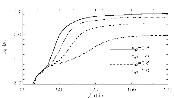
4.6.6.2 Viscosity
An important difference between edge dominated modes and the already well-studied vortex modes in planetary gaps is the effect of viscosity on them. The standard viscosity prevents vortex mode development, but §4.2 showed that such viscosity values still allow the edge modes to develop. Vortices are localised disturbances and more easily smeared out than global spirals in a given time interval. Hence, vortex growth is inhibited more easily by viscosity than spirals.
The run was repeated with a range of viscosities. Results are shown in Fig. 4.22. Generally, lowering viscosity increases the amplitudes of the non-axisymmetric modes. For , the mode emerges first (note that this is not in conflict with linear calculations which used in its basic state), rather than . This is because lowering viscosity allows a sharper vortensity peak to develop in the background model, and thus has the same effect as increasing the disc mass. The latter generally enable higher edge modes.
Unlike vortex modes, even with twice the standard viscosity () the edge mode develops and grows. It is only suppressed when . However, this is because no vortensity maxima could be setup at the gap edges due to vortensity diffusion in the co-orbital region making an almost uniform vortensity distribution in the gap (e.g. the final plot in Fig. 4.17). Since the necessary condition for edge modes is not achieved, no linear modes exist. This differs from the nature of the suppression of vortex modes, because in that case vortensity extrema can still be setup.

4.7 Applications to disc-planet interactions
In order to focus on the issue of gap stability, the planet was held on a fixed orbit. However, torques exerted by the non-axisymmetric disc on the planet will induce migration that could occur on a short time scale (Pepliński et al., 2008b, e.g.). Such torques will be affected by the presence of edge modes.
4.7.1 Disc-planet torques
The presence of large-scale edge mode spirals of comparable amplitude as the planetary wake will significantly modify disc-on-planet torques. Here, this torque is measured while still keeping the planet on fixed orbit. This eliminates torques due to migration.
Fig. 4.23(a) shows the evolution of the torque per unit length for the fiducial case. The torque profile at before the edge modes have developed significantly, shows the outer torque is larger in magnitude than inner torque, implying inward migration. This is a typical result for disc-planet interactions and serves as a reference. At and , edge modes mostly modify the torque contributions exterior to the planet, though some disturbances are seen in the interior disc (, recall is the Hill radius). The original outer torque at , is reduced in magnitude as material re-distributed to concentrate around the co-rotation radius of the edge mode ( is away from the planet).
Edge modes can both enhance or reduce disc-planet torques associated with planetary wakes. Consider in Fig. 4.23(a). Comparing the situation at to that at , the torque contribution from this region is seen to be more negative. This is because an edge mode spiral overlaps the planetary wake and therefore contributes an additional negative torque on the planet. However, at , an edge mode spiral is just upstream of the planet, exerting a positive torque on the planet, hence the torque contribution from becomes positive.
Differential rotation between edge modes and the planet produces oscillatory torques, shown in Fig. 4.23(b). Unlike typical disc-planet interactions, which produce inward migration, the total instantaneous torques in the presence of edge modes can be of either sign. For a disturbance with fold symmetry the time interval between encounters with the planet is , where is the difference in angular velocity of the planet and the disturbance pattern. Approximating with obtained from linear theory gives . Indeed, the oscillation period in Fig. 4.23 is . Both inner and outer torques oscillate, but since the edge mode is more prominent in the outer disc, oscillations in the outer torque are larger, particularly after mode saturation ().


Time-averaged torques are compared in Fig. 4.23(c). In all three disc masses, on average a negative torque acts on the planet and its magnitude largest at . Up to this point, the torque becomes more negative as the disc mass increases, as expected. However, development of edge modes makes the averaged torques more positive, and eventually reverses the trend with . While the disc with also attains steady torque values as in , the disc with has significant oscillations even after time-averaging and is remains non-steady at the end of the run.
Before the instability sets in, torques arise from wakes induced by the planet, and the outer (negative) torque is dominant. Edge modes concentrate material into spiral arms, leaving voids in between. Therefore, except when spiral arms cross the planet’s azimuth, the surface density in the planetary wake is reduced because it resides in the void in between edge mode spirals. Hence the torque magnitude is reduced. If the reduction in surface density due to voids in between edge mode spirals is greater than the increase in surface density scale produced by decreasing the presence of edge modes will, on average make the torque acting on the planet more positive.
4.7.2 Outward scattering by spiral arms
If edge modes develop, planetary migration may be affected by them. Their association with gap edges inevitably affects co-orbital flows. The more long term effect of edge modes on migration is explored in Chapter 5. This subsection highlights an interesting effect found when edge modes are present. This is outward migration induced by spiral arms analogous to vortex-induced rapid migration described in Chapter 2.
Some of the simulations described above were restarted at allowing the planet to move in response to the gravitational forces due to the disc. Fig. 4.24 shows the orbital radius of the planet in discs with edge modes present. No obvious trend with can be seen. This is because of oscillatory torques (positive or negative) due to edge modes and the partial gap associated with a Saturn mass planet, which is associated with type III migration (Masset & Papaloizou, 2003). The initial direction of migration can be inwards or outwards depending on the relative positioning of the edge mode spirals with respect to the planet at the time the planet was first allowed to move.
Outward migration is seen for and For , the planet migrates by , or 8.6 times its initial Hill radius, within only This is essentially the result of a scattering event. Repeating this run with tapering applied to contributions to disc torques from within of the planet, outward scattering still occurs, but limited to and the planet remains at until . Hence, while the subsequent inward migration seen for may be associated with conditions close to the planet, the initial outward scattering is due to an exterior edge mode spiral.
For the planet is scattered to . It is interesting to note that the subsequent inward migration for and stalls at , i.e. the original outer gap edge. The planet remains there for sufficient time for both gap and edge mode development and for a second episode of outward scattering occurs. Interaction with edge modes can affect the disc well beyond the original co-orbital region of the planet. In the case of outward migration, it may promote gravitational activity in the outer disc. However, boundary effects may be important after significant outward scattering.

The spiral arm-planet interaction for above is detailed in Fig. 4.25. A spiral arm approaches the planet from the upstream direction () and exerts positive torque on the planet, increasing . The gap is asymmetric in the azimuthal direction with the surface density upstream of the planet being larger than that downstream of the planet (). As the spiral arm passes through the planetary wake (—) the gap surface density just ahead of the planet builds up as an edge mode is setup across the gap. Notice the fluid blob at . This signifies material executing horseshoe turns ahead of the planet. At the later time the planet has exited the original gap, in which the average surface density is now higher than before the scattering. Material that was originally outside the gap loses angular momentum and moves into the original gap. This material is not necessarily that composing the spiral.
Migration through scattering by spiral arms differs from vortex scattering. Vortices form about vortensity minima, which lie further from the planet than vortensity maxima. Vortensity maxima are stable in the case of vortex formation. This means the ring of vortensity maxima must be disrupted in order for vortices to flow across the planet’s orbital radius for direct interaction. Edge modes themselves correspond to a disruption of vortensity maxima, hence direct interaction is less hindered than in the vortex case. Furthermore, a vortex is a material volume of fluid. Vortex-planet scattering results in an orbital radius change of both objects. However, a spiral pattern is generally not a material volume of fluid. It can be seen in Fig. 4.25 that the local in the spiral remains at approximately the same radius before and after the interaction. The spiral pattern as a whole does not move inwards. In this case, the spiral first increases the planet’s orbital radius, thereby encouraging it to interact with the outer gap edge and scatter that material inwards.


4.8 Summary and discussion
The investigation of planetary gap stability has been extended to massive protoplanetary discs. Vortex instabilities, associated with local vortensity minima, have previously been found to occur in weakly or non self-gravitating discs. However, edge modes that are associated with local vortensity maxima and require sufficiently strong self-gravity were found in the more massive discs in this Chapter. These have very different properties in that they are global rather than local and are associated with large scale spiral arms as well as being less affected by viscous diffusion.
For the disc-planet models here, with fixed planet mass and fixed disc aspect-ratio , edge modes develop for gap profiles with an average Toomre exterior to the planet’s orbital radius. In the unperturbed smooth disc, this corresponds to at the planet’s location and at the outer boundary, or equivalently a disc mass . For fixed , nonlinear simulations show edge modes develop readily for uniform kinematic viscosity and self-gravitational softening .
A theoretical description of edge modes was developed. The edge mode is interpreted as a disturbance associated with an interior vortensity maximum that requires self-gravity to be sustained, and which further perturbs the remainder of the disc through its self-gravity causing the excitation of density waves. These density waves acts to destabilise the edge disturbance. Linear calculations confirm this picture and also show the expected strengthening of the instability when self-gravity is increased via the disc mass and the expected weakening of the instability through increasing gravitational softening.
Hydrodynamic simulations of disc-planet interactions confirm earlier suggestions by Meschiari & Laughlin (2008), who found gravitational instabilities associated with prescribed gap profiles without a planet. Indeed, edge modes can develop for gaps self-consistently opened by introducing a planet into the disc. However, models here showed their development during gap formation of a Saturn-mass planet, when the gap only consists of a — deficit in surface density relative to the unperturbed disc. This is much shallower than the Jovian-mass planetary gaps considered in Meschiari & Laughlin (2008). Edge modes exist for the disc models considered here with masses , again this is less massive than required in Meschiari & Laughlin (2008), but more massive than those typically used in modelling protoplanetary discs.
Simulations show edge modes with and They have surface density maxima localised near the outer gap edge, but the disturbance they produce extends throughout the entire disc, consistent with analytical expectation and linear calculations. One important difference between edge modes and the vortex forming modes in non-self-gravitating discs is that the latter require low viscosity. The typical viscosity values adopted for protoplanetary discs, , will suppress vortex formation but not edge modes around a gap opened by a Saturn-mass planet.
Edge modes produce large oscillations in the disc torques acting on the planet, which can be positive or negative. The presence of edge modes reverses the trend of the time averaged disc-on-planet torque as a function of disc mass: the torque being more positive as disc mass increases. Direct interaction between the planet and a spiral arm associated with an edge mode is possible. These should be more prominent in the disc section with the lower In practise this corresponds to so the planet tends to interact with the outer spirals, which results in a scattering of the planet outwards.
Chapter 5 Planetary migration in the presence of edge modes
Edge modes significantly modify disc-planet torques from the classic picture of monotonic inwards migration in low-mass discs. Hence, migration of gap-opening planets in massive protoplanetary discs is expected to be qualitatively different to that in gravitationally stable discs. For example, §4.7.2 indicate the possibility of direct gravitational interaction with an edge mode spiral arm. This is analogous, although distinct, from vortex-planet scattering.
This Chapter explores the effect of edge modes associated with gap edges on planetary migration averaged over timescales much longer than that for scattering. Torque measurements from fixed-orbit simulations in Chapter 4 show the time-averaged disc-on-planet torques become more positive with disc mass. For Saturn-mass planets this effect is due to modification of Lindblad torques. However, for the Jovian mass planets adopted here, edge modes were found to supply torques from a region very close to the planet’s orbital radius.
This study is fully numerical and is organised as follows. The disc-planet model is described in §5.1 and their stability discussed in §5.2. Simulation results are presented in §5.3 and a fiducial case is analysed in §5.4. §5.5 concludes this Chapter with a discussion of the implications of the results.
5.1 Simulation setup
The class of disc profiles are identical to that used in Chapter 3—4. The discs are two-dimensional and are parameterised by their Keplerian Toomre value at the outer boundary, , or equivalently the disc-to-star mass ratio . These are chosen via the surface density scale. The discs have uniform kinematic viscosity .
The disc spans and a larger planetary mass is considered. This opens a deep gap so that strong scattering with spiral arms leading to large jumps in orbital radius on orbital timescales, do not occur. It allows one to examine the long term effect of edge modes averaged over many orbits. Numerically, a larger is advantageous because there are more cells per Hill radius than smaller .
The planet is introduced on a circular orbit at , this is further from disc boundaries than in disc-planet models used previously. This attempts to reduce boundary effects, should the planet move significantly.
5.1.1 Equation of state
The equation of state is locally isothermal, so the vertically integrated pressure is where is a specified function. However, as noted in Chapter 3, adopting (as used in most of the previous simulations) in a self-gravitating disc means the planet mass is no longer a free parameter. The effective planet mass is plus disc material gravitationally bound to the planet. This effect will be significant for Jovian mass planets. To reduce it, one can artificially increase near the planet by using the EOS described in §1.18. The parameter in this EOS controls the temperature increase relative to the profile, and is fixed at . Far away from the planet, the disc aspect-ratio is fixed at and the temperature profile returns to . The motivation in using this EOS is entirely numerical.
5.1.2 Numerics
The disc is divided into zones in radius and azimuth, logarithmically and uniformly spaced respectively. The resolution is approximately 16 cells per (or 28 cells per ). The cells are nearly square (). Open boundaries are applied at the inner boundary and non-reflecting at the outer boundary, as before. The self-gravity softening is .
The planet is introduced with zero mass at . Its mass is then switched on smoothly over to its final value . The planet is then allowed to respond to disc gravitational forces for . A standard fifth order Runge-Kutta scheme is used to integrate its equation of motion. The softening length for the planet potential is .
5.2 Disc models and their stability
Four discs are presented here to assess the stability of the adopted models: . These correspond to a Toomre parameter at the planet’s initial radius of and total disc masses of , respectively. The discs are gravitationally stable to axisymmetric perturbations. For smooth radial profiles, they are also expected to be gravitationally stable to non-axisymmetric perturbations near because .
Fig. 5.1 shows the surface density perturbation for the disc models when the planet mass reaches its final value. The gap structure is similar and relatively stable. The over-density at the outer gap edge upstream of the planet () resembles an edge mode. However, this is likely associated with the introduction of a massive planet over a short time-scale, rather than instability of an axisymmetric gap. This is because it is present in all disc masses with the same azimuthal wavenumber (), whereas the most unstable edge mode is expected to be of higher with increasing disc mass. This transient feature increases in magnitude with , and for it visibly makes the gap less clean.


For stability discussion, one dimensional gap profiles should be used, because linear analysis is usually applied to axisymmetric backgrounds. Fig. 5.2 compares the azimuthally averaged surface density perturbation and Toomre profiles at . The gap is almost cleared (). The surface density perturbation is similar to that induced by a Saturn-mass planet, apart from the spike near due to disc material bound to the planet. As expected, this causes the gap edges to become more steep with lowering .
The fundamental quantity for stability is the vortensity . The edge mode is associated with , which for gap profiles coincide with . Fig. 5.2 shows that edge mode corotation should occur inside the gap. Assuming the coorbital region of a giant planet is (Artymowicz, 2004b; Paardekooper & Papaloizou, 2009), is just within the outer gap edge. This suggests the development of edge modes could bring over-densities into the coorbital region of the planet.
Edge modes also require coupling to the outer smooth disc, which is easier with lower . Interestingly, in Fig. 5.2 the profile beyond the outer gap edge becomes smoother as is reduced. The local at the outer gap edge is most pronounced for , which favour vortex modes. The profiles here indicate edge modes will develop more readily with increasing disc mass and therefore have more significant effect on migration as is lowered.


5.2.1 Fragmentation of high mass discs
Giant planets can induce fragmentation in marginally stable discs. This phenomenon was previously identified in smooth particle hydrodynamic simulations by Armitage & Hansen (1999) and Lufkin et al. (2004). However, grid-based codes are generally better at resolving shocks and therefore planetary wakes. Fig. 5.1 confirms that planetary wakes may become gravitationally unstable as a clump forms along the outer wake in .
Fig. 5.3 shows that fragmentation indeed occur for within of releasing the planet, and there is no annular gap. This means that for very massive discs (), migration will be significantly affected by these clumps, rather than large-scale spirals associated with edge modes.


5.3 Migration and disc structure
Edge modes lead to non-axisymmetric over-densities inside the gap. This is a potential source for torques to originate from within the planet’s coorbital region. Because is expected near the outer edge of the coorbital region, edge mode over-densities may undergo horseshoe turns upon approaching the planet. Furthermore, fluid elements just inside the separatrix will traverse close to the planet when it executes the U-turn, and this may provide significant torque.
Fig. 5.4 shows the instantaneous orbital radius of the planet in non-fragmenting disc models. Migration is non-monotonic and can be inwards or outwards on short time-scales (). However, with increasing disc mass, outwards migration is favoured on timescales of a few 10’s of orbits. For , increases by in only .

The behaviour of correlates with the coherence of the gap structure. Fig. 5.5 shows that first develops vortex mode (with ). Although a viscosity of suppressed vortex modes in previous studies (for ), increasing has the same effect as lowering , hence vortex modes are not completely suppressed. does develop spiral arms later on, but these probably result from the vortices perturbing the disc, rather than the linear edge mode instability. The important feature with is that instability leaves the gap edge intact and identifiable, unlike more massive discs below. Related to this is that Fig. 5.6 shows up to , the torque magnitudes for are typically smaller than in that .


develops a —3 edge mode, making the gap less well-defined. The chosen snapshot is just prior to a small outwards jump in for (Fig. 5.4) and Fig. 5.6 shows a clear positive disc-on-planet torque at this instant. Fig. 5.5 shows that the over-density inside the gap and associated with the edge mode, just upstream of the planet, could provide such positive torque. The outer gap edge in is not as disrupted and this results in no secular increase in over the simulated timescale.
In Fig. 5.5, large-scale spirals can still be seen for . Weak fragmentation occurs but collapse into clumps are not seen. Like , the gap is unclean, but now with significant disruption to the outer gap edge. It is no longer a clear feature like in .

5.3.1 Gap evolution
The migration curves in Fig. 5.4 results from modification to the gap structure by instabilities. The following prescription was used to monitor gap structure. A one-dimensional profile of the relative surface density perturbation is first calculated (as in Fig. 5.2). The outer gap edge is defined as such that there, and similarly for the inner gap edge . The outer gap depth is averaged over . The outer gap width, in units of the Hill radius, is and the inner gap width is . The gap asymmetry is . Running time-averaged () plots are shown in Fig. 5.7
Edge modes have a gap-filling effect. The case , in which the planet immediately migrates outwards, has the smallest gap depth throughout. has the deepest gap and is non-migrating over the simulation timescale. In , the magnitude of gap depth decreases relative to that for after . Note that this corresponds to outwards migration in . These observations suggests that material brought into the gap by edge modes, is responsible for outwards migration.
Gap asymmetry was defined as the distance from the planet to the outer gap edge minus the distance between the planet and the inner gap edge. It follows that the more negative gap asymmetry is, the closer the planet is to the outer gap edge. Fig. 5.7 shows the planet is located closer to the outer gap edge in discs with lower than in discs with higher . Furthermore, the non-migrating reaches a constant asymmetry, whereas in the outwards-migrating cases asymmetry decreases with time.
The trend above suggests that the planet is moving material associated with the outer gap edge, which is unstable to edge modes, inwards via horseshoe turns (this would also be consistent with shallower gaps with decreasing ). This provides a positive torque on the planet. If, on average, this effect dominates over sources of negative torques, e.g. negative Lindblad torques and the enhancement of which by the coincidence of an edge mode spiral arm with the outer planetary wake, then the planet should on average migrate outwards, i.e. closer to the outer gap edge.


5.4 A fiducial case in detail
Fig. 5.8 and Fig. 5.9 presents a summary of the simulation with , in terms of the evolution of the planet’s orbit and the disc’s surface density perturbation. The orbit remains fairly circular with no secular change in eccentricity. However, the semi-major axis increases more noticeably than orbital radius .
Fig. 5.9 shows the outer disc () is unstable to edge modes whereas the inner disc () remains relatively stable. Large-scale spirals are maintained throughout the simulation. The gap is unclean with material brought into it by the edge modes. Notice in the and snapshots the over-density just upstream and exterior to the planet. It resides within the planet’s coorbital region () so this material is expected to execute inwards horseshoe turns and exert a positive torque on the planet. If this torque is sufficiently large, it may trigger type III migration because it promotes the planet to move closer to the higher density gap edge and interact with it. This can explain the faster-than-linear increase in . In this case the edge mode over-densities provides the coorbital mass deficit.


5.4.1 Torques and mode amplitudes
Fig. 5.10 shows the time-averaged evolution of non-axisymmetric modes in the outer disc, together with evolution of disc-on-planet torques. The effect of edge modes can be seen by comparison to the non-migrating case . The modes have larger amplitudes in , and the total torque becomes more positive with time11 1 The total torque values are negative, despite overall outwards migration, because the running time-average is plotted. The average includes the time at planet release, when the disc-planet torque is large negative. . The figure shows this is attributed to torques from within the Hill radius, which is positive. By contrast, although also develop large-scale spirals later on, they are of smaller amplitude and do not make the Hill torque positive. The total time-averaged torque remains fairly constant.
Fig. 5.10, along with Fig. 5.9, confirms that large-scale spirals which extend into the gap can provide significant torques. Edge modes naturally fit this description since they are associated with vortensity maxima just inside the gap. Because the outer disc is more unstable, the corotation radius of edge modes lie beyond so its pattern speed is smaller than the planet’s rotation. Thus, over-densities associated with corotation approach the planet from upstream, but because is actually within the planet’s coorbital region, the associated fluid elements are expected to execute (inwards) horseshoe turns upon approaching the planet. This provides a positive torque on the planet, and if the edge mode amplitude is large enough, it may reverse the usual tendency for inwards migration.
The picture outlined above is consistent with the fact that edge modes have corotation at vortensity maxima. A giant planet can induce shocks very close to its orbital radius (Chapter 2) and vortensity is generated as fluid particles execute horseshoe turns across the shock. That is, the vortensity rings are associated with particles on horseshoe orbits. So when non-axisymmetric disturbances associated with vortensity rings develop (i.e. edge modes), the associated over-densities can be expected to execute horseshoe turns.


5.4.2 Torque distribution
The analysis above suggests that torques from within the gap are responsible for the gradual increase in or . Fig. 5.11 compares torque densities in the fiducial case to the non-migrating case. The torques have been averaged over at two time intervals. For radial plots for both cases show a positive torque at . By this torque has diminished for . This is expected for Jovian planets as they open a clean gap, leaving little material near to torque the planet. However, in , this torque is maintained (and even slightly increased) by the edge modes because they bring material into the co-orbital region.
Azimuthal plots in Fig. 5.11 only account for material in between the gap edges (quantitatively defined in §5.3.1). Both cases have similar distributions for . For though, the torque becomes symmetric about the planet’s azimuth for , whereas for asymmetry is maintained, leading to a positive torque. This torque is caused by over-density ahead in comparison to that behind the planet, i.e. material flowing radially inwards across the planet’s orbital radius. However, unlike the single scattering events by vortices or spirals, which dominate most of the migration, here migration occurs on much longer timescales in comparison.


5.5 Summary and discussion
The numerical experiments above have shown that edge modes can induce outwards migration over timescales of a few tens of initial orbital periods. In the planet’s frame, an edge mode spiral, with corotation at vortensity maximum exterior to , approaches the planet from . However, the mode extends into the planet’s coorbital region, so there are associated over-densities that execute inwards horseshoe turns, which provides a positive torque.
The torque responsible for outwards migration can be identified as positive bump at in the time-averaged radial torque plots in Fig. 5.11, resulting from azimuthal gap asymmetry about the planet. This torque diminishes with time in the non-migrating case, thus migration itself helps to maintain this torque. Note that such torque was also absent in the Saturn-mass case when held on fixed orbit (Fig. 4.23). Another difference to Saturn is Jovian mass planets induce larger perturbations and the gap-filling effect of edge modes tend to be stronger.
Edge modes must be sustained in order to provide this torque, this in turn requires the existence of vortensity maximum, despite the development of edge modes destroying them. However, this is easily regenerated by giant planets because they induce shocks which act as a source of vortensity. Furthermore, since edge modes also require gravitational coupling to an exterior smooth disc, outwards migration of this type is probably more likely to occur than inwards, because typically discs become more self-gravitating with increasing radius.
Planetary migration observed here closely resembles classic type III migration (Masset & Papaloizou, 2003) because it relies on torques from the coorbital region and the accelerated increase in semi-major axis indicate positive feedback. The main difference to type III migration originally described by Masset & Papaloizou is that the flow across the planet’s orbit is non-smooth, because edge modes present distinct fluid blobs, rather than a continuous flow across . Also, where type III migration usually apply to partial gaps and therefore Saturn-mass planets, the Jovian mass planet used here reside in a much deeper gap. Radial mass flux across the planet is still possible, despite the gap-opening effect of Jovian planets, because the unstable edge modes brings over-densities inside the gap to interact with the planet.
A consequence of the above is that formation of a clean gap is expected to become increasingly difficult in massive discs. Planetary gaps correspond to existence of vortensity maximum, but these become unstable to edge modes in massive discs and instability tends to fill the gap. In very massive discs giant planets induce fragmentation, their planetary wakes become gravitationally unstable and no annular gap forms. Therefore classic type II migration, where the planet moves smoothly with the viscous gap evolution, probably does not apply in massive discs.
5.5.1 Outstanding issues
It should be noted that the adopted disc model is biased towards outwards migration because the Toomre decreases outwards (approximately like ) so edge modes associated with the outer disc develops preferentially. If a disc model such that the inner disc is more unstable was used, then inwards migration should occur. And if independent edge modes of comparable amplitude develop on either side of the gap, there should be little migration overall.
Significant torques originate from material close to the planet, so numerical treatment of the Hill sphere is a potential issue. This concern also applies to standard type III migration, but note that the adopted equation of state was originally designed for numerical studies of type III migration (Pepliński et al., 2008a). Furthermore, fully self-gravitating discs are suited for type III migration (Crida et al., 2009). Lower resolution simulations have been performed which also resulted in outwards migration.
This EOS mimics heating near the planet but is not a quantitative model for the true thermodynamics. If this EOS under-estimates the heating, then the positive torque could be over-estimated and vice versa. On the other hand, edge mode corotation reside outside the Hill radius but still inside the gap. So the numerical treatment of the Hill radius does not affect existence of edge modes and their associated over-densities should affect torques originating from the coorbital region in the way described in this Chapter.
Chapter 6 Three-dimensional simulations
Razor-thin discs have been used in all the previous numerical simulations. This approximation can be justified for gap-opening planets, whose definition can be taken as , so that the planet’s Hill radius exceeds the local disc thickness. Nevertheless, three-dimensional discs should be considered because instabilities studied above are associated with radial structures with characteristic length scales comparable to the local thickness.
In this Chapter, numerical simulations are developed to confirm properties of gap stability studied previously in 2D, persist in 3D geometry. The 3D disc-planet models are presented in §6.1. §6.2 describes adaptation of the ZEUS-MP software to perform disc-planet simulations with and without disc self-gravity. Three-dimensional counterparts to previous 2D results are presented in §6.3, including vortex formation and vortex-induced migration in non-self-gravitating discs, vortex modes in self-gravitating discs and edge modes in massive discs. §6.4 concludes this Chapter.
6.1 Three-dimensional models
The governing equations for three-dimensional discs are listed in Chapter 1. The disc model is extended from that used in Chapter 3—5 by introducing vertical structure. The disc is described in spherical polar co-ordinates with origin on the central star, is now the spherical polar radius, and the cylindrical radius denoted by and the cylindrical .
The disc occupies , and . The vertical extent is such that corresponds to number of scale-heights. The initial density profile is
| (6.1) |
where is the scale-height with the fixed aspect-ratio, is a constant parameterising the density scale. The power-law index in surface density is fixed at for all the simulations performed. Recall is the stellar potential. Eq. 6.1 results from exact vertical hydrostatic equilibrium assuming an isothermal equation of state with sound-speed . As before, the density scale is chosen via the Keplerian Toomre parameter at the outer boundary:
| (6.2) |
Note that vertical integration in Eq. 6.2 corresponds to the computational domain so exterior mass is either zero or assumed negligible. Thus models with fixed but increasing will have decreasing midplane density scale represented by .
The disc is initialised without meridional velocity () and azimuthal velocity given by centrifugal balance between stellar potential and pressure:
| (6.3) |
Exact balance implies , but since the disc is thin (), the azimuthal velocity is well approximated to be Keplerian ( ).
6.1.1 Self-gravity
The three-dimensional disc potential is obtained by solving the differential Poisson equation . This removes the need for a softening length used for 2D self-gravity. However, boundary conditions must be explicitly imposed and will be described in §6.2.
Instead of solving for the initial vertical structure consistent with self-gravity, a simpler numerical approach is taken. All calculations are initialised with the non-self-gravitating equilibrium described above. To account for radial self-gravity, the initial azimuthal velocity is reset to . The vertical self-gravity force, , is initially set to zero and then smoothly increased to its full value over time.
6.1.2 Planet treatment and equation of state
The planet potential is softened by a fraction of its Hill radius
| (6.4) |
The softening is set to . In 2D, softening by a fraction of the local scale-height approximately accounts for vertical structure, whereas softening in 3D is purely to avoid numerical divergence. The Hill radius is calculated with , but this is very close to the planet’s cylindrical radius from the star because the orbit inclination is negligible for all the migrating cases presented later. The planet is introduced on fixed circular orbit of radius in the midplane with Keplerian rotation speed and its mass is smoothly switched on.
The disc-on-planet forces are tapered by multiplying all components of the force by the factor . The cut-off parameter is set to unity unless otherwise stated. Tapering is applied whether or not disc self-gravity is enabled. Without self-gravity, the physical motivation for tapering is that material close to the planet should be gravitationally bound to it and should be excluded in the disc-on-planet force. There is no physical need for tapering in a self-gravitating disc, but limited numerical resolution in a 3D calculation prevents accurate determination of torques from close to the planet. Thus, the tapering is largely motivated by numerics.
The equation of state is isothermal, so the pressure is . Before introducing the planet, is the locally isothermal sound-speed giving the standard Gaussian atmosphere. After the planet is introduced, the sound-speed is modified to given by Eq. 1.18 which heats up the disc near the planet relative to the profile. This prescription is used to limit mass pile-up near the planet and reduce numerical errors resulting from this effect. It also helps to reduce the increase in effective planet mass and therefore the effect of self-gravity on instabilities through the background planetary gap.
6.2 Adapting ZEUS-MP
ZEUS is a general-purpose astrophysical fluid dynamics code based on finite-difference schemes. Several versions are publicly available11 1 http://lca.ucsd.edu/portal/software, including ZEUS-2D (Stone & Norman, 1992a; Stone & Norman, 1992b; Stone et al., 1992) which FARGO is based on, and its three-dimensional version ZEUS-3D. The version adapted here is ZEUS-MP , developed and described by Hayes et al. (2006), which places emphasis on parallel computing. ZEUS-MP is capable of solving hydrodynamics, self-gravity, magnetohydrodynamics and radiative transfer, although the latter two modules are disabled in this study.
6.2.1 Source terms
The most important new source term is the gravitational forces on disc fluid due to the planet potential. The acceleration is added directly to to the momentum equations to update each velocity component () as part of the source term step in ZEUS-MP . Indirect disc and planet potentials are also added, to account for the non-inertial reference frame.
All simulations presented have zero physical viscosity (artificial viscosities is employed by ZEUS-MP to treat shocks). However, a module for viscous forces has also been added to ZEUS-MP . Velocity components can be updated by the full viscous stress tensor immediately after the main source step. The magnitude of the viscous force is characterised by kinematic viscosity , which can be a constant or , where is a constant. The effect of viscosity on vortex and edge modes in 3D is not expected to differ to that in 2D discs, which has already been investigated.
6.2.2 Disc potential
ZEUS-MP was chosen for its ability to solve 3D self-gravity in spherical polar co-ordinates with parallelisation. This is an uncommon feature among public codes. The discretised Poisson equation is a linear system, . ZEUS-MP solves this using the conjugate gradient (CG) method (see Hayes et al., 2006, for details). It is an iterative scheme that minimises the quadratic form . At the iteration, the CG method finds the scalar and conjugate direction (such that if ) to give the improved solution as (Press et al., 1992; Barrett et al., 1994, e.g.).
6.2.2.1 Boundary potential
A potential solver based on Boss (1980) has been added to ZEUS-MP to obtain potentials at - and -boundaries, which are set as Dirichlet boundary conditions for the CG solver. The potential is periodic in . The potential and density are expanded in spherical harmonics, so that
| (6.5) |
In practice the sum is truncated at and . To further reduce computation cost, only even modes are used, corresponding to symmetry with respect to the disc midplane. is found by direct integration:
| (6.6) |
This integration is parallelised by domain decomposition along with the hydrodynamics. Each processor holds a copy of the global but performs the integration over its local sub-domain of the global disc. The result is written to the appropriate sub-portion of the global . A global reduction is then performed, summing contributions to from all angles that is held on different processors.
After expansion, the Poisson equation becomes
| (6.7) |
where , and radial boundary conditions
| (6.8) |
are applied. The discretised version of Eq. 6.7 is a tridiagonal matrix equation. It can be solved relatively quickly with the LAPACK software package to yield . The potential at and boundaries can be found from Eq. 6.5. Note that the solution method outline here assumes no mass outside the computational domain.
6.2.3 Planetary migration
Planetary migration is mostly neglected in order to focus on the issue of gap stability. However, a fifth order Runge-Kutta integrator (Press et al., 1992) for the equation of motion of the planet has been implemented in ZEUS-MP . During one hydrodynamic time step , the planet’s position and velocity is integrated from with adaptive sub-steps but using the density field at . If only the upper disc () is simulated, then the vertical force is set to zero and the planet remains in the midplane.
6.3 Gap stability in 3D
The substantial cost of a 3D numerical calculation prevent extensive parameter studies. Instead, described below are specific simulations demonstrating gap instability. The general numerical setup is as follows.
The disc is divided into zones in the directions, uniformly spaced in and logarithmically spaced in polar . During the disc is evolved without the planet. Between , the planet mass is switched on. If the disc is self-gravitating then for , is set for the boundary potential and is smoothly switched on. For , is set for the boundary potential. Hydrodynamic boundary conditions are outflow in radius, reflecting in and periodic in .
6.3.1 Vortex instability in a non-self-gravitating disc
In this simulation the disc model is . The domain is and scale-heights above and below the midplane. The resolution is , corresponding to cells per in , but only cells per in and . The planet mass is and is fixed in the midplane at radius after its introduction. The EOS parameter is .
Fig. 6.1 show density perturbations relative to the azimuthally-averaged density field at . Two cuts in are shown, corresponding to the midplane and at . The vortex instability clearly persists for planetary gaps in a three-dimensional disc. The relative density perturbation has no vertical dependence (except near the planet since it is embedded). This is also seen in the three-dimensional plot in Fig. 6.2. Since the background density is essentially Gaussian in , the vortex density field will also be Gaussian vertically.


The evolution is very similar to 2D discs simulated in Chapter 2—3. The only noticeable difference is that in 2D without self-gravity, 3 vortices develop initially then merge (Fig. 3.7). In the 3D run, one vortex develops from the beginning (although a weak, second vortex can be identified in Fig. 6.1 at ). Reduction in the number of vortices from 2D to 3D was also noted by Meheut et al. (2010). However, in quasi-steady state the vortex in 3D and 2D are essentially identical. These results show that the vortex instability is a 2D instability . Thus, the condition for instability can be largely determined by vertically integrated properties of the disc.
The vortex vertical structure is shown in Fig. 6.3. The vortex lies just outside the outer gap edge at . Its associated relative density and vortensity perturbations have very weak vertical dependence, despite the background being Gaussian. Stratification has no effect on the instability.


The mass flux of the main vortex at is drawn in Fig. 6.4 for several meridional planes. As expected for an anticyclonic vortex, the radial flow transits from inwards to outwards as one traverses anti-clockwise (increasing ) through the vortex. The transition point is the vortex centroid. The slice shows that the transition involves vertical flux, but its magnitude is small even near the midplane, where the mass density is largest. This means the vortex centroid has very little motion. There is no evidence for strong meridional circulation found by Meheut et al. (2010), but the flow towards the midplane highlighted in Fig. 6.4 suggest vertical motion near the vortex centroid, as seen in Meheut et al.. Note that symmetry about is broken, so mass flux can overshoot across the midplane.


6.3.2 Vortex-planet interaction
Fig. 6.5 shows the planet orbital radius after it is released at for the simulation in §6.3. Also shown is a second simulation where only was simulated and the planet released at (before vortices fully develop). Results are very similar to 2D, the migration composing of slow and rapid phases, the latter induced by the vortex associated with the inner gap edge. Since the interaction is gravitational, and the perturbed density field associated with the vortex has no vertical structure, it is not surprising that the same interaction occurs in 3D as in 2D.

6.3.3 Vortex modes with self-gravity
For 3D self-gravitating simulations, the computational domain is and . For simulations in this subsection the resolution is . Jovian planets are used to open the gap because the steeper edges imply higher growth rates than gaps opened by a Saturn-mass planet. This shortens the simulation time. The planet is fixed at and simulated up to . The EOS parameter is .
Fig. 6.6 compares vortex formation in the disc models, with . It confirms that the effect of self-gravity on the vortex instability discussed in Chapter 3, persists in 3D. Comparing the outer gap edge at shows self-gravity is stabilising, because in vortices can already be identified but not so readily seen in . At , more vortices develop with lowering because stabilisation is more effective for low , thus higher vortex modes are favoured, just as in 2D. The 6-vortex and 5-vortex configuration remains in , respectively, at whereas only 3 remain in (reduced from 4). This is due to resisted merging as vortices behave like co-orbital planets with increasing self-gravity. Again, this was seen in 2D.


The vertical structure of a vortex in the disc is shown in Fig. 6.7. Because the initial disc is not in self-gravitating equilibrium, the density perturbation relative to and to (just after is fully switched on) are both shown. The increasing perturbation towards the midplane is partly due to vertical self-gravity increasing the background midplane density. Between and there may also be additional stratification due to vertical self-gravity of the vortex, since the midplane density is largest. Stratification is reduced if perturbation is taken relative to , so the instability indeed tends to involve the entire column of fluid.
The vortensity field in Fig. 6.7 shows some disturbance along the contour lines at the vortex boundary, as well as closed contours within the vortex, which is associated with anti-clockwise motion indicated by mass flux vectors in Fig. 6.8. Meheut et al. (2010) found similar flow to occur in pairs — clockwise () and anti-clockwise (), where denotes the vortex centroid. Such symmetry may not be expected here since there is a planet located on one side of the gap edge. It is also likely that the flow here has been modified by self-gravity of the vortex and/or background. However, despite additional vertical structure and flow, the vortensity perturbation remains largely columnar.


6.3.4 Edge modes
The disc model is used to demonstrate edge modes. The resolution is increased to , on account of reduction in effective scale-height due to vertical self-gravity.
Fig. 6.9 shows the development of an edge mode and Fig. 6.10 is a three-dimensional visualisation. Perturbations are calculated relative to . The behaviour near the midplane is similar to 2D simulations, but the edge mode amplitude decreases noticeably away from the midplane. The background density () near has been reduced by vertical self-gravity from . This means that perturbations high in the atmosphere appear enhanced, but their actual densities are small compared to the midplane.


Fig. 6.11—6.12 shows the vertical structure of the edge mode near the gap edge. The density perturbation is even more stratified than a self-gravitating vortex . Most of the disturbance is contained within and the corresponding vortensity perturbation is no longer columnar. Mass flux goes into the over-density radially from either side, as well as vertically from above. Since the density perturbation in the midplane is large (up to —3 times over-dense than the background), this blob of fluid perturbs the surrounding flow gravitationally. The vertical flux is likely attributable to this effect. Recall that the vertical boundaries are solid, so flow must reflect off it.


6.3.5 Outwards migration induced by edge modes
This simulation is the 3D version of the fiducial case in Chapter 5. The disc model is and the resolution is . is reduced to enable longer simulation times. The planet mass is now and it is allowed to migrate for . Since torques originating from close to the planet were found to be important in the 2D simulations, the torque cut-off parameter is reduced to (about 3.5 cells).
Fig. 6.13 and Fig. 6.13 shows the migration history and snapshots of density perturbation. These figures can be compared to the 2D case, Fig. 5.8—5.9. Whereas the 2D disc developed –3 edge modes, only was seen in 3D. This could be due to the much reduced resolution in 3D (by a factor of 4 in and compared to 2D), or reduction in the strength of self-gravity due to disc thickness.

Despite the low resolution, this simulation demonstrates that edge modes can induce outwards migration in 3D discs. Outwards migration only begins around after release, whereas it starts immediately in the 2D run. The migration in 3D is also on average slower than in 2D. This is probably because the applied tapering (for numerical considerations) artificially reduces the torque magnitudes. However, the existence of edge modes does not depend on treatment close to the planet. Their development will likely bring material into the gap for interaction with the planet, because they are associated with the gap edge. This is shown in Fig. 6.14, which is qualitatively very similar to the 2D run. The planet is asymmetrically positioned with respect to gap edges. Edge mode spiral arms protrude into the gap and supply an over-density within the coorbital region of the planet upstream to it. As the spiral pattern pass by from to , edge mode material in the planet’s coorbital region is expected to execute inward horseshoe turns ahead of the planet. This contributes positively to the disc-on-planet torque.


6.4 Summary and discussion
The first 3D numerical simulations demonstrating planetary gap instability were presented. The instabilities behave similarly in 2D and 3D. In retrospect, 2D is a better approximation for self-gravitating discs than for non-self-gravitating discs because vertical self-gravity compresses the midplane.
The vertical structure of the vortex instability was first studied in non-self-gravitating discs by Meheut et al. (2010). They found prominent circulatory flow in the plane, but these features are not seen in the current simulations. However, Meheut et al. used prescribed disc profiles which lead to strong instability (growth rate ) whereas profiles here are induced by a planet, for which 2D linear calculations gave smaller growth rates (a few per cent of ). There could also be influences from the planet. Simulations here show vortices and edge mode spirals have increasing vertical dependence as the strength of self-gravity is increased. This is probably due to additional vertical acceleration due to self-gravity by the higher midplane density.
Computational cost present significant obstacle to 3D simulations. Vortices and edge modes are global instabilities associated with localised gradients. Thus entire discs must be simulated whilst maintaining good resolution locally. In the 3D runs here, resolution in is only 4—6 cells per , compared to 16 in 2D simulations. Improved resolution and a convergence study should be performed in the future. Despite numerical limitations, the similarity between 3D and 2D results validates the razor-thin disc approximation employed in previous Chapters. In fact, it may be more advantageous to use 2D in some situations, e.g. massive discs and planet migration, because high resolution is achievable. Migration should only depend on the density field, which has essentially the same structure in 2D and 3D.
Chapter 7 Conclusions and future work
7.1 Main results
7.1.1 Unstable gap structure
Planetary gaps are characterised by thin vortensity rings outlining its edges. They are generated across shocks induced by the planet. Their formation can be anticipated from models of the planet-perturbed flow and expected shock location. For planetary masses of Saturn or above, these shocks extend well into the gap and the rings reside in the planet’s co-orbital region. The existence of vortensity extrema satisfies the necessary condition for instability.
7.1.2 Vortex modes and induced migration
In a low viscosity, non-self-gravitating disc, corotation radii of unstable modes are associated with local vortensity minima at gap edges. Their nonlinear outcome is the formation of a few vortices that merge on dynamical timescales. The result is one azimuthally-extended vortex circulating just outside either gap edge.
For the standard disc models adopted, differential Lindblad torques favour inwards migration and lead to gravitational scattering of the inner vortex outwards. The planet therefore receives an inwards kick of a few Hill radii. Migration alternates between a slow phase, when gap and vortex formation takes places, and brief rapid inward jumps.
The role of vortices in such non-smooth migration can be understood as a modified form of type III migration. Vortices provide a coorbital mass deficit when it is circulating on the gap edge, and remove it when they flow across the gap and fill it to some extent.
7.1.3 Effect of self-gravity on vortex modes
Increasing self-gravity is stabilising for the vortex mode, if the background disc profile remains fixed. However, in practice the effective planetary mass increases with the strength of self-gravity due to disc material bound to the planet. This results in steeper gap edges with increasing surface density scales, and this destabilises the vortex mode.
The combined effect of self-gravity through the background profile and through the linear response is to shift the most unstable vortex mode to higher azimuthal wave-numbers. This leads to more vortices with increasing disc mass. These self-gravitating vortices are localised in azimuth as well as radius, and they can behave like co-orbital planets. Their mutual gravitational interaction allows them to survive against vortex merging for a longer period of time than in non-self-gravitating discs.
7.1.4 Edge modes in massive discs
The vortex mode is suppressed in sufficiently massive discs. Instead, unstable modes have co-rotation radii at local vortensity maximum, which lie closer to the planet than vortensity minimum. These edge modes can be interpreted as a disturbance associated with the gap edge, which induces activity in the smooth part of the disc via self-gravity. Thus they are global modes. For the disc models adopted here, they are seen predominantly as one-sided spiral arms in the disc beyond the planet’s orbital radius.
Edge modes associated with the outer gap edge make the disc-on-planet torque on average more positive than that in stable discs.Outwards migration is thus promoted. A Saturn-mass planet can be scattered by an edge mode spiral and jump outwards significantly on orbital timescales. More massive Jovian planets reside in deeper gaps but can migrate outwards on timescales of 10’s of orbits. These effects originate from material brought into the gap by the edge mode.
7.1.5 Validity of razor-thin discs
The use of 2D discs to study planetary gap stability has been validated by counterpart 3D numerical simulations. Vortex modes and edge modes behave similarly in both geometries. Not surprisingly, the vertical dependence of their structure increases with the strength of self-gravity.
7.2 Directions for future work
Attention has mostly been placed on understanding the phenomenon found in each of the preceding Chapters. The trade-off is the realism of disc models and the size of parameter space that can be practically surveyed. Extensions to this work are listed below.
7.2.1 Three-dimensional linear calculations
Although the non-self-gravitating 3D simulations did not reproduce vertical structure found by Meheut et al. (2010), it is clear that vortices involve vertical motion. In order to gain a better understanding of three-dimensional effects, if any, it would be ideal to have 3D linear stability analysis to complement nonlinear simulations.
A simple starting point would be three-dimensional, locally isothermal discs with radial structure, such as a surface density bump (Li et al., 2000, e.g. profiles used by). The vertical structure is Gaussian, so if the disc occupies , one can expand the vertical dependence of perturbations as , where is the Hermite polynomial. would represent the 2D solution and would be the first 3D contribution to an even vortex mode. This leads to the system of coupled first order ODE’s analysed by Tanaka et al. (2002), but the problem here would be solving for the homogeneous solution, with eigenfrequencies to be determined. Preliminary results show that 3D has negligible effect on growth rates and, e.g. , so perturbations are indeed columnar. Nonetheless, the small vertical velocities still grow exponentially and this should be important in the nonlinear regime.
However, it is more realistic to have finite vertical boundaries, particularly for the vortex modes. This is because they are easily suppressed by viscosity, and would only exist in ‘dead zones’ of protoplanetary discs which have sufficiently low viscosity. However, dead zones exist close to the disc midplane and do not occupy the entire vertical extent (Gammie, 1996). In this case one requires the solution to a 2D partial differential equation eigenvalue problem.
7.2.2 Planet-edge mode interactions
Systematic studies of planetary migration in massive discs have only begun recently (Michael et al., 2011; Baruteau et al., 2011c). These first simulations consider disc masses of . Such discs are gravitationally active even without a planet.
Lower mass discs that are gravitationally stable without a planet can become gravitationally active via edge modes associated with planetary gaps. Edge mode properties depend on planetary properties, but the unstable disc has significant back-reaction on planet migration, which could subsequently affect further edge mode development. An example is edge mode-induced migration moving the planet to a region even more prone to edge modes.
These inter-dependencies will be explored with high resolution 2D numerical simulations. This is an expansion of Chapter 5, which focused on the migration mechanism, to a parameter survey. Questions include the relation between planet and disc masses that allow edge modes, and how the extent of migration depend on planetary and disc properties.
7.2.3 Numerical simulations with ZEUS-MP
Three-dimensional simulations in Chapter 6 were primarily performed to confirm 2D results. Future numerical studies with ZEUS-MP will focus on properties of vortex and edge modes in 3D self-gravitating discs.
Further development of ZEUS-MP is needed. Currently, the non-self-gravitating initial conditions are evolved towards equilibrium. This inevitably leaves disturbances in the disc , relative to which perturbations are defined. Although subsequent perturbations due to planet, vortices and edge modes are much larger than the noise in the background, it would be ideal to have a module to to generate clean initial discs in equilibrium with self-gravity. Development of polytropic disc models is also planned, as a preliminary step towards including thermodynamics, which is important for gravitational instabilities.
Many interesting issues arise in 3D. The vertical structure of vortex and edge modes as a function of gap properties should be investigated. Vertical boundary conditions (including the treatment of the gravitational potential in terms of ) may be important for vortex modes because they tend to involve entire fluid columns, i.e. they are global in . The evolution of 3D self-gravitating disc vortices, including the possibility of self-gravitational collapse, vortex merging (a phenomenon common in 2D) and their migration (Paardekooper et al., 2010a, so far only simulated in 2D by) should be studied. These numerical works require improved numerical resolutions.
Chapter 8 Upper limit on the horseshoe width
It is possible to place an upper limit on the horseshoe width that is valid in the limit of either zero or constant pressure. Consider a local Cartesian frame that has origin at the planet and hence co-rotates with it with the Keplerian angular velocity The direction corresponds to increasing radius and is azimuthal direction (same sense as ). In this frame, consider fluid elements approaching the planet from with velocity Suppose such a fluid element executes a horseshoe turn crossing the co-orbital radius at position with velocity . The maximum value of , below which such motions occur, is determined as follows.
The equation of motion governing a fluid element or particle, in the absence of pressure forces, is
| (8.1) |
where
| (8.2) |
contains contributions from the gravitational potential of the planet of mass (with the softening length neglected) and the tidal potential associated with the central object. From Eq. 8.1 it follows that the Jacobi invariant
| (8.3) |
is constant along a particle path. Equating evaluated at to evaluated at gives
| (8.4) |
The steady-state Euler equation of motion for evaluated at is
| (8.5) |
In the neighbourhood of for the type of streamline being considered, and because the particle is going from to by executing a U-shape turn. This implies
| (8.6) |
Combining Eq. 8.4 and Eq. 8.6 gives
| (8.7) |
Writing and in units of the Hill radius, i.e. setting and , gives
| (8.8) |
Thus because the maximum possible value of the right hand side of the above is particles executing a U-turn could not have originated further than from the planet’s orbital radius. This is comparable to the value of that has been estimated from hydrodynamic simulations (Artymowicz, 2004b; Paardekooper & Papaloizou, 2009).
Appendix 8.A Application to co-orbital vortices
It is straight forward to apply the equations above to describe gravitational interaction between two vortices in the shearing sheet. The equations have exactly the same form, with a slight change of notation where denote the relative displacement of the two vortices in the shearing sheet frame. becomes the sum of vortex masses. The frame is now centred on one of the vortices, its average orbital radius from the central star being .
Non-dimensionalising by , Eq. 8.7 becomes
| (8.A1) |
where , , and the angular speed of the rotating frame has been used. Eq. 8.A1 relates the initial mutual radial separation of the vortex pair, , to their minimum azimuthal separation, .
Eq. 8.A1 is useful for the case there vortices are just able to undergo U turns. For fixed , the function
| (8.A2) |
has a maximum value at corresponding to the maximum conceivable initial separation where
| (8.A3) |
If then Eq. 8.A1 cannot be satisfied and there can be no mutual horseshoe turns (as in the test particle and planet case). For initial separations , Eq. 8.A1 implies that the minimal inter-vortex distance (in ) must exceed (so that ). Now for sufficiently large will be larger than the critical separation for merging (set by hydrodynamics), so merging is avoided during the encounter.
It is interesting to compare Eq. 8.A3 to the estimate of the horseshoe half-width of Paardekooper & Papaloizou (2009). They found based on hydrodynamic simulations for low mass planets. Equating and with gives This should give the minimum for which pressure effects could be ignored. Inserting this value in Murray & Dermott (2000)’s model of coorbital satellites gives a minimal separation of (with other parameter values estimated in §3.5.4), which is close to simulation results (Fig. 3.21). Hence, if the vortex-pair interaction in Chapter 3 is purely gravitational, a single vortex behaves in a similar way to Earth masses, i.e. a low-mass protoplanet.
Considering a vortex size of order , the vortex-to-star mass ratio is . For a self-gravitating vortex where the Toomre , for , slightly exceeding the threshold value above. Hence the pressureless treatment of self-gravitating vortex-vortex interactions should be acceptable for the purpose of explaining the resisted-merging of self-gravitating vortices.
Chapter 9 Linear model for flow perturbed by a planet
When modelling the pre-shock flow in the presence of a planet (§2.3.1), the pressureless momentum equations were integrated directly. Here, a simple linear model for the pre-shock velocity field is presented, which was found to give qualitatively correct results compared to hydrodynamic simulations.
Low mass planets cannot have shocks close to because flow is purely azimuthal and becomes subsonic close to the planet (in the planet’s frame). The goal of this calculation is to introduce non-zero radial velocity by treating the planet potential as a perturbation. The planet mass is assumed to be sufficiently small to allow linearisation, but large enough to ignore pressure. The zero-pressure, steady state momentum equations in the shearing sheet are
| (9.1) | ||||
| (9.2) |
The centre of the frame co-rotates with the planet. Linearising about the Keplerian flow
| (9.3) | ||||
| (9.4) |
where denote small Eulerian perturbations, gives
| (9.5) | ||||
from the -momentum equation. The linearised -momentum equation is:
| (9.6) | ||||
Eliminating gives
| (9.7) |
where . Eq. 9.7 is an ODE with as a parameter. Multiplying by and considering the limit ( ) demands the balance:
| (9.8) |
which implies, from Eq. 9.6, that close to ,
| (9.9) |
The expression for is equivalent to Eq. 28 of Paardekooper & Papaloizou (2009) when pressure is neglected, and is equivalent to their Eq. 30 if is neglected.
Eq. 9.7 describes a forced oscillator and solutions are readily obtained by writing
| (9.10) |
and imposing
where the prime denotes . For , the coefficients are written as
| (9.11) | ||||
| (9.12) |
So that as for fixed . The part of the forcing can be integrated by parts (twice) to give explicit velocity expressions
| (9.13) | ||||
| (9.14) | ||||
The second line for follows from Eq. 9.6 once are known, and this is the expression used in practice. Since , linearisation fails for small .
The planet-perturbed velocity field is now available for use. To first approximation, let the velocity field be , i.e. the -velocity perturbation is neglected in comparison to Keplerian flow. The unperturbed uniform density field, , is assumed when the surface density is needed. Taking the shock front from simulation data, Fig. 9.1 compares shock strength predicted by the above calculation to that found in disc-planet simulations. The linear solution over-estimates but its position of maximum, at (for respectively) is close to simulation results. In particular, the curve follows closely to simulation. This simple linear calculation adequately predicts the qualitative behaviour of along a given shock. More importantly it confirms the planet-induced enable shocks near , and that vortensity is generated within about a Hill radius from the planet (which is the region of increasing with respect to ).
Fig. 9.2 compare vortensity jumps. Linear theory under-estimates vortensity generation, probably because and the unperturbed uniform density was used, which is larger than the actual pre-shock surface density (this is seen in Fig. 2.4 as diverging particle paths approaching the U-turn). The agreement between the linear model and simulation is better in , in terms of position of maximum vortensity jump and shock strength, since linearisation become better approximation as decreases (despite the pressureless approximation becoming worse).


Chapter 10 Shocks induced by a planet and the vorticity jump across it
Appendix 10.A Estimating shock fronts
Papaloizou et al. (2004) presented a method based on characteristic rays to estimate the shape of wakes induced by a planet. It was applied to Keplerian flow. Their formalism is outlined below and applied to general two-dimensional flow. Note that the method applies to local or global frames.
Consider a frame which rotates at the planet’s fixed circular orbital frequency. The hydrodynamic variables are assumed to have wave-like spatial and time dependencies, , where is a wavenumber and a frequency. Seeking a local dispersion relation from the hydrodynamic equations yields
| (10.A1) |
The wavefronts or characteristic curves are related to the dispersion relation by
| (10.A2) | ||||
where is the non-dimensional velocity and similarly for . The second line in Eq. 10.A2 applies the dispersion relation Eq. 10.A1, and the third line follows by defining .
The solution of interest is the characteristic ray with , corresponding to a stationary wave in the planet frame. Setting the frequency to zero, Eq. 10.A1 reads:
| (10.A3) |
which is a quadratic equation for with solution
| (10.A4) |
where . Using Eq. 10.A3 to replace in Eq. 10.A2 gives
| (10.A5) |
Finally, inserting the expression for from Eq. 10.A4 gives
| (10.A6) | ||||
| (10.A7) |
which can be solved once a flow field is given. The solution correspond to wakes induced by the planet, with the minus (plus) sign corresponding to wakes exterior (interior) to the planet. These wakes develop into shocks for sufficiently large planetary masses.
Appendix 10.B Vorticity jump across a steady isothermal shock
Consider an isothermal shock that is stationary in a frame rotating with angular velocity . In order to evaluate the vorticity jump across the shock it is convenient to use a two dimensional orthogonal coordinate system defined in the disc mid-plane such that one of the curves coincides with the shock. The curves will then be normal to the shock where they intersect it. In addition the coordinates are set up so that is a right handed system. This co-ordinate system is depicted in Fig.10.1 where distances along the normal () and tangential () directions to the shock are labelled respectively.
The -component of relative vorticity can then be written as
| (10.B1) |
where are the components of the coordinate scale factor.
Note that on is the velocity tangential to the shock and is unchanged across the shock. The normal component and other state variables undergo a jump from pre-shock values to post-shock values on normally traversing the curve For an isothermal shock
| (10.B2) |
where is the pre-shock perpendicular Mach number. Here and in similar expressions below connecting pre-shock and post-shock quantities, post-shock values are denoted with a subscript post while pre-shock quantities are left without a corresponding subscript. Thus the jump in relative vorticity is
| (10.B3) |
Quite generally the component of the equation of motion for a steady state flow is
| (10.B4) |
or equivalently
| (10.B5) |
where is the pressure and the total potential (the latter quantity being continuous across the shock). From Eq. 10.B5, the relative vorticity can be written in the form
| (10.B6) |
Applying Eq. 10.B6 to give an expression for the post shock relative vorticity, and using Eq. 10.B2 to express the post-shock normal velocity and density in terms of the corresponding pre-shock quantities, the vorticity jump can be written in the form
| (10.B7) |
where continuity of across the shock has been used in the pressure term. Adopting a locally isothermal equation of state implies Substituting this into Eq. 10.B7, while making use of Eq. 10.B6 together with the relation gives
| (10.B8) |
where is the absolute vorticity.
Setting with being the corresponding element of distance measured parallel to the shock, this takes the form
| (10.B9) |
This gives the vorticity jump across a shock in terms of pre-shock quantities measured in the rotating frame in which it appears steady. It is important to note that Eq. 10.B9 applies specifically in the right handed coordinate system adopted with shock location given by If instead was adopted for this location, the signs of the derivative terms would be reversed as in the expression (2.23) given in Kevlahan (1997). Note too that the last term on the right hand side that is proportional to the gradient of along the shock arises from the assumption of a locally isothermal equation of state and is not present in the treatment given by Kevlahan (1997).

Chapter 11 Approximate equations in linear calculations
The full governing equation for linear perturbations in a self-gravitating disc with fixed temperature profile was summarised in Chapter 3 as
| (11.1) |
An expression for the linear operator is given by Eq. 3.33. The eigenvalue is contained in as in a complicated manner. However, once appearances of as denominators are removed by multiplying Eq. 11.1 by the appropriate factor, one can neglect various powers of , to approximate the above equation in quadratic and linear order in .
Appendix 11.A Governing equation to
In the quadratic approximation, the governing equation is
| (11.A1) |
where
| (11.A2) | ||||
| (11.A3) | ||||
| (11.A4) |
The operators are:
| (11.A5) | ||||
| (11.A6) | ||||
| (11.A7) | ||||
| (11.A8) |
The operators are defined by Eq. 3.34.
Appendix 11.B Governing equation to
The approximation for corotational or vortex modes made in Chapter 2 can also be recast in a standard eigenvalue form as above. Recall that in this approximation, is only retained when it appears as associated with the vortensity gradient term. In other words, and . The simplified equation is then
| (11.B1) |
where
| (11.B2) | ||||
| (11.B3) |
Self-gravity was neglected in Chapter 2, in which case the operators are set to zero.
Chapter 12 Artificial vortices in an accretion disc
The artificial Kida-like vortices used in §3.5 were set up by introducing velocity perturbations that correspond to the elliptical vortices of Kida (1981) in an incompressible shear flow.
Consider a small patch of the disc, whose centre rotates at angular speed about the primary and set up local Cartesian co-ordinates . In the frame, there exists a Kida vortex solution for incompressible flow, whose velocity field is
| (12.1) |
inside the vortex core. The ratio of the vortex semi-major to semi-minor axis being is a free parameter. This velocity field is such that the vorticity is constant in the rotating frame. The elliptical boundary of the vortex is defined such that inside the boundary of the vortex and outside. The quantity is then the vorticity of the vortex core relative to the background. Being negative, this corresponds to an anticyclonic vortex. In order to introduce perturbations corresponding to Kida vortices, perturbations are introduced inside a specified elliptical boundary with an exponential decay outside. The boundary is fixed by specifying and semi-major axis where the reference radius is .
Chapter 13 Energy densities in linear theory of edge modes
In order to understand edge modes, in §4.5 the thermal-gravitational energy (TGE) was defined and the different contributions to it were discussed. There, a factor was applied to the TGE per unit length and to each contributing term in order to overcome numerical difficulties associated with Lindblad resonances. For completeness, the behaviour of the TGE and the various contributions to it is considered here without the additional factor
Fig. 13.1 shows very smilier features to the corresponding curves discussed in §4.5.2. is negative around corotation, again signifying a self-gravity driven edge mode. Beyond , becomes positive due to pressure. The most extreme peak at coincides with the background vortensity edge (Fig. 4.5). The negative contribution from the corotation term is larger in magnitude than that from the positive wave term, resulting in . The co-rotation radius is such that , making the shifted frequency . Also at , , resulting in at this point.

and have relatively small spurious bumps around that are associated with the outer Lindblad resonance and are numerical. The eigenfunctions are well-defined without singularities there, but evaluating and involves division by , which can amplify numerical errors at Lindblad resonances where . Integrating over gives The TGE is negative, which means gravitational energy dominates over the pressure contribution for . Integrating the contributions to the TGE separately gives
The integration range includes the OLR and thus the spurious bumps in and However, still approximately equals . The correct energy balance is maintained despite being subject to possible numerical error due to the diverging factor The above means that, aside from the spurious bumps, the energy density values for may still be used to interpret energy balance. As as before, the TGE is predominantly accounted for by the vortensity term, since .
References
- Adams et al. (1989) Adams, F. C., Ruden, S. P., & Shu, F. H. 1989, ApJ, 347, 959
- Armitage (2010) Armitage, P. J. 2010, ArXiv e-prints
- Armitage & Hansen (1999) Armitage, P. J., & Hansen, B. M. S. 1999, Nature, 402, 633
- Artymowicz (1993) Artymowicz, P. 1993, ApJ, 419, 155
- Artymowicz (2004a) Artymowicz, P. 2004a, in Astronomical Society of the Pacific Conference Series, Vol. 324, Debris Disks and the Formation of Planets, ed. L. Caroff, L. J. Moon, D. Backman, & E. Praton, 39–+
- Artymowicz (2004b) Artymowicz, P. 2004b, in KITP Conference: Planet Formation: Terrestrial and Extra Solar
- Balbus & Hawley (1991) Balbus, S. A., & Hawley, J. F. 1991, ApJ, 376, 214
- Balmforth et al. (2001) Balmforth, N. J., Cunha, M. S., Dolez, N., Gough, D. O., & Vauclair, S. 2001, MNRAS, 323, 362
- Barrett et al. (1994) Barrett, R., et al. 1994, Templates for the Solution of Linear Systems: Building Blocks for Iterative Methods, 2nd Edition (Philadelphia, PA: SIAM)
- Baruteau et al. (2011a) Baruteau, C., Cuadra, J., & Lin, D. N. C. 2011a, ApJ, 726, 28
- Baruteau et al. (2011b) Baruteau, C., Fromang, S., Nelson, R. P., & Masset, F. 2011b, ArXiv e-prints
- Baruteau & Masset (2008) Baruteau, C., & Masset, F. 2008, ApJ, 678, 483
- Baruteau et al. (2011c) Baruteau, C., Meru, F., & Paardekooper, S.-J. 2011c, MNRAS, 1086
- Boss (1980) Boss, A. P. 1980, ApJ, 236, 619
- Bracco et al. (1999) Bracco, A., Chavanis, P. H., Provenzale, A., & Spiegel, E. A. 1999, Physics of Fluids, 11, 2280
- Bryden et al. (1999) Bryden, G., Chen, X., Lin, D. N. C., Nelson, R. P., & Papaloizou, J. C. B. 1999, ApJ, 514, 344
- Chavanis (2000) Chavanis, P. H. 2000, A&A, 356, 1089
- Crida et al. (2009) Crida, A., Baruteau, C., Kley, W., & Masset, F. 2009, A&A, 502, 679
- Crida et al. (2006) Crida, A., Morbidelli, A., & Masset, F. 2006, Icarus, 181, 587
- D’Angelo et al. (2005) D’Angelo, G., Bate, M. R., & Lubow, S. H. 2005, MNRAS, 358, 316
- D’Angelo et al. (2010) D’Angelo, G., Durisen, R. H., & Lissauer, J. J. 2010, Giant Planet Formation, ed. Seager, S., 319–346
- de Val-Borro et al. (2007) de Val-Borro, M., Artymowicz, P., D’Angelo, G., & Peplinski, A. 2007, A&A, 471, 1043
- de Val-Borro (2006) de Val-Borro, M. e. 2006, MNRAS, 370, 529
- Durisen et al. (2007) Durisen, R. H., Boss, A. P., Mayer, L., Nelson, A. F., Quinn, T., & Rice, W. K. M. 2007, Protostars and Planets V, 607
- Fu & Lai (2011) Fu, W., & Lai, D. 2011, MNRAS, 410, 399
- Gammie (1996) Gammie, C. F. 1996, ApJ, 457, 355
- Gammie (2001) —. 2001, ApJ, 553, 174
- Godon (1996) Godon, P. 1996, MNRAS, 282, 1107
- Goldreich & Tremaine (1979) Goldreich, P., & Tremaine, S. 1979, ApJ, 233, 857
- Goldreich & Tremaine (1980) —. 1980, ApJ, 241, 425
- Hawley (1987) Hawley, J. F. 1987, MNRAS, 225, 677
- Hayashi (1981) Hayashi, C. 1981, Progress of Theoretical Physics Supplement, 70, 35
- Hayes et al. (2006) Hayes, J. C., Norman, M. L., Fiedler, R. A., Bordner, J. O., Li, P. S., Clark, S. E., ud-Doula, A., & Mac Low, M. 2006, ApJS, 165, 188
- Kevlahan (1997) Kevlahan, N.-R. 1997, J. Fluid Mech., 341, 371
- Kida (1981) Kida, S. 1981, Journal of the Physical Society of Japan, 50, 3517
- Klahr & Bodenheimer (2003) Klahr, H. H., & Bodenheimer, P. 2003, ApJ, 582, 869
- Kley & Dirksen (2006) Kley, W., & Dirksen, G. 2006, A&A, 447, 369
- Kocsis et al. (2011) Kocsis, B., Yunes, N., & Loeb, A. 2011, Phys. Rev. D, 84, 024032
- Koller et al. (2003) Koller, J., Li, H., & Lin, D. N. C. 2003, ApJ, 596, L91
- Korycansky & Papaloizou (1995) Korycansky, D. G., & Papaloizou, J. C. B. 1995, MNRAS, 274, 85
- Lesur & Papaloizou (2009) Lesur, G., & Papaloizou, J. C. B. 2009, A&A, 498, 1
- Li et al. (2001) Li, H., Colgate, S. A., Wendroff, B., & Liska, R. 2001, ApJ, 551, 874
- Li et al. (2000) Li, H., Finn, J. M., Lovelace, R. V. E., & Colgate, S. A. 2000, ApJ, 533, 1023
- Li et al. (2005) Li, H., Li, S., Koller, J., Wendroff, B. B., Liska, R., Orban, C. M., Liang, E. P. T., & Lin, D. N. C. 2005, ApJ, 624, 1003
- Li et al. (2009) Li, H., Lubow, S. H., Li, S., & Lin, D. N. C. 2009, ApJ, 690, L52
- Lin & Papaloizou (1986) Lin, D. N. C., & Papaloizou, J. 1986, ApJ, 309, 846
- Lin & Papaloizou (1993) Lin, D. N. C., & Papaloizou, J. C. B. 1993, in Protostars and Planets III, ed. E. H. Levy & J. I. Lunine, 749–835
- Lin et al. (1993) Lin, D. N. C., Papaloizou, J. C. B., & Kley, W. 1993, ApJ, 416, 689
- Lin & Papaloizou (2010) Lin, M.-K., & Papaloizou, J. C. B. 2010, MNRAS, 405, 1473
- Lin & Papaloizou (2011a) —. 2011a, MNRAS, 415, 1426
- Lin & Papaloizou (2011b) —. 2011b, MNRAS, 415, 1445
- Lissauer & Stevenson (2007) Lissauer, J. J., & Stevenson, D. J. 2007, Protostars and Planets V, 591
- Lovelace & Hohlfeld (1978) Lovelace, R. V. E., & Hohlfeld, R. G. 1978, ApJ, 221, 51
- Lovelace et al. (1999) Lovelace, R. V. E., Li, H., Colgate, S. A., & Nelson, A. F. 1999, ApJ, 513, 805
- Lufkin et al. (2004) Lufkin, G., Quinn, T., Wadsley, J., Stadel, J., & Governato, F. 2004, MNRAS, 347, 421
- Lynden-Bell & Ostriker (1967) Lynden-Bell, D., & Ostriker, J. P. 1967, MNRAS, 136, 293
- Lynden-Bell & Pringle (1974) Lynden-Bell, D., & Pringle, J. E. 1974, MNRAS, 168, 603
- Lyra et al. (2009) Lyra, W., Johansen, A., Zsom, A., Klahr, H., & Piskunov, N. 2009, A&A, 497, 869
- Marcy et al. (2005) Marcy, G., Butler, R. P., Fischer, D., Vogt, S., Wright, J. T., Tinney, C. G., & Jones, H. R. A. 2005, Progress of Theoretical Physics Supplement, 158, 24
- Masset (2000a) Masset, F. 2000a, A&AS, 141, 165
- Masset (2000b) Masset, F. S. 2000b, in Astronomical Society of the Pacific Conference Series, Vol. 219, Disks, Planetesimals, and Planets, ed. G. Garzón, C. Eiroa, D. de Winter, & T. J. Mahoney, 75–+
- Masset (2002) Masset, F. S. 2002, A&A, 387, 605
- Masset (2008) Masset, F. S. 2008, in EAS Publications Series, Vol. 29, EAS Publications Series, ed. M.-J. Goupil & J.-P. Zahn, 165–244
- Masset & Papaloizou (2003) Masset, F. S., & Papaloizou, J. C. B. 2003, ApJ, 588, 494
- Mayor & Queloz (1995) Mayor, M., & Queloz, D. 1995, Nature, 378, 355
- McKernan et al. (2011) McKernan, B., Ford, K. E. S., Lyra, W., Perets, H. B., Winter, L. M., & Yaqoob, T. 2011, ArXiv e-prints
- Meheut et al. (2010) Meheut, H., Casse, F., Varniere, P., & Tagger, M. 2010, A&A, 516, A31+
- Melander et al. (1988) Melander, M. V., Zabusky, N. J., & McWilliams, J. C. 1988, Journal of Fluid Mechanics, 195, 303
- Meschiari & Laughlin (2008) Meschiari, S., & Laughlin, G. 2008, ApJ, 679, L135
- Michael et al. (2011) Michael, S., Durisen, R. H., & Boley, A. C. 2011, ApJ, 737, L42+
- Murray & Dermott (2000) Murray, C. D., & Dermott, S. F. 2000, Solar System Dynamics
- Nelson & Benz (2003) Nelson, A. F., & Benz, W. 2003, ApJ, 589, 556
- Nelson & Papaloizou (2004) Nelson, R. P., & Papaloizou, J. C. B. 2004, MNRAS, 350, 849
- Ou et al. (2007) Ou, S., Ji, J., Liu, L., & Peng, X. 2007, ApJ, 667, 1220
- Paardekooper et al. (2010a) Paardekooper, S., Lesur, G., & Papaloizou, J. C. B. 2010a, ApJ, 725, 146
- Paardekooper et al. (2010b) Paardekooper, S.-J., Baruteau, C., Crida, A., & Kley, W. 2010b, MNRAS, 401, 1950
- Paardekooper et al. (2011) Paardekooper, S.-J., Baruteau, C., & Kley, W. 2011, MNRAS, 410, 293
- Paardekooper & Mellema (2006) Paardekooper, S.-J., & Mellema, G. 2006, A&A, 459, L17
- Paardekooper & Mellema (2008) —. 2008, A&A, 478, 245
- Paardekooper & Nelson (2009) Paardekooper, S. J., & Nelson, R. P. 2009, ArXiv e-prints
- Paardekooper & Papaloizou (2009) Paardekooper, S.-J., & Papaloizou, J. C. B. 2009, MNRAS, 394, 2297
- Papaloizou & Savonije (1991) Papaloizou, J. C., & Savonije, G. J. 1991, MNRAS, 248, 353
- Papaloizou (2005) Papaloizou, J. C. B. 2005, Celestial Mechanics and Dynamical Astronomy, 91, 33
- Papaloizou & Lin (1989) Papaloizou, J. C. B., & Lin, D. N. C. 1989, ApJ, 344, 645
- Papaloizou et al. (2006) Papaloizou, J. C. B., Nelson, R. P., Kley, W., Masset, F. S., & Artymowicz, P. 2006, Protostars and Planets V, 655
- Papaloizou et al. (2007) Papaloizou, J. C. B., Nelson, R. P., Kley, W., Masset, F. S., & Artymowicz, P. 2007, in Protostars and Planets V, ed. B. Reipurth, D. Jewitt, & K. Keil, 655–668
- Papaloizou et al. (2004) Papaloizou, J. C. B., Nelson, R. P., & Snellgrove, M. D. 2004, MNRAS, 350, 829
- Papaloizou & Pringle (1984) Papaloizou, J. C. B., & Pringle, J. E. 1984, MNRAS, 208, 721
- Papaloizou & Pringle (1985) —. 1985, MNRAS, 213, 799
- Papaloizou & Pringle (1987) —. 1987, MNRAS, 225, 267
- Papaloizou & Terquem (2006) Papaloizou, J. C. B., & Terquem, C. 2006, Reports on Progress in Physics, 69, 119
- Pepliński et al. (2008a) Pepliński, A., Artymowicz, P., & Mellema, G. 2008a, MNRAS, 386, 164
- Pepliński et al. (2008b) —. 2008b, MNRAS, 386, 179
- Pepliński et al. (2008c) —. 2008c, MNRAS, 387, 1063
- Petersen et al. (2007a) Petersen, M. R., Julien, K., & Stewart, G. R. 2007a, ApJ, 658, 1236
- Petersen et al. (2007b) Petersen, M. R., Stewart, G. R., & Julien, K. 2007b, ApJ, 658, 1252
- Pierens & Huré (2005) Pierens, A., & Huré, J.-M. 2005, A&A, 433, L37
- Press et al. (1992) Press, W. H., Teukolsky, S. A., Vetterling, W. T., & Flannery, B. P. 1992, Numerical recipes in FORTRAN. The art of scientific computing
- Sellwood & Kahn (1991) Sellwood, J. A., & Kahn, F. D. 1991, MNRAS, 250, 278
- Shakura & Sunyaev (1973) Shakura, N. I., & Sunyaev, R. A. 1973, A&A, 24, 337
- Stone et al. (1992) Stone, J. M., Mihalas, D., & Norman, M. L. 1992, ApJS, 80, 819
- Stone & Norman (1992a) Stone, J. M., & Norman, M. L. 1992a, ApJS, 80, 753
- Stone & Norman (1992b) —. 1992b, ApJS, 80, 791
- Tanaka et al. (2002) Tanaka, H., Takeuchi, T., & Ward, W. R. 2002, ApJ, 565, 1257
- Tassoul (1978) Tassoul, J. 1978, Theory of rotating stars
- Toomre (1964) Toomre, A. 1964, ApJ, 139, 1217
- Udry & Santos (2007) Udry, S., & Santos, N. C. 2007, ARA&A, 45, 397
- Uribe et al. (2011) Uribe, A. L., Klahr, H., Flock, M., & Henning, T. 2011, ApJ, 736, 85
- Ward (1997) Ward, W. R. 1997, Icarus, 126, 261
- Weidenschilling (1977) Weidenschilling, S. J. 1977, MNRAS, 180, 57
- Yu & Li (2009) Yu, C., & Li, H. 2009, ApJ, 702, 75
- Yu et al. (2010) Yu, C., Li, H., Li, S., Lubow, S. H., & Lin, D. N. C. 2010, ApJ, 712, 198
- Zabusky et al. (1979) Zabusky, N. J., Hughes, M. H., & Roberts, K. V. 1979, Journal of Computational Physics, 30, 96
- Zhang et al. (2008) Zhang, H., Yuan, C., Lin, D. N. C., & Yen, D. C. C. 2008, ApJ, 676, 639