Isomorphism of graph classes related to the circular-ones property
Abstract
We give a linear-time algorithm that checks for isomorphism between two matrices that obey the circular-ones property. This algorithm leads to linear-time isomorphism algorithms for related graph classes, including Helly circular-arc graphs, circular-arc graphs, proper circular-arc graphs and convex-round graphs.
1 Introduction
Two graphs and are isomorphic if there is a bijection from the vertex set of to the vertex set of that satisfies the following condition: for all , is adjacent to in if and only if is adjacent to in . The graph isomorphism problem consists of determining whether two input graphs are isomorphic. The graph isomorphism problem is in , but it is neither known to be NP-complete nor known to be in . However, the restriction of the problem to members of graph classes with certain special topological properties is known to result in polynomial or even linear-time algorithms. The subject of this paper is the development of such algorithms for a variety of such classes.
We show linear-time isomorphism algorithms for Helly circular-arc graphs, circular-arc graphs, proper circular-arc graphs and convex-round graphs. The common building block for all of these algorithms, is a linear-time isomorphism algorithm for binary matrices that obey the circular-ones property, which we show.
In order to explain our results, we first establish some basic terminology. A matrix is a binary matrix if all of its entries are 0 or 1. The adjacency matrix of a simple graph is a binary square matrix that has in row , column , if vertex is adjacent to vertex , and 0 otherwise. The augmented adjacency matrix of is the adjacent matrix of the graph with ’s on the main diagonal.
A clique matrix of a graph is a binary matrix that has one row for each vertex and one column for each maximal clique, and a 1 in row , column if vertex is a member of maximal clique .
A consecutive-ones matrix is a binary matrix whose columns can be ordered such that, in every row, the 1’s are consecutive. Such an ordering of the columns is a consecutive-ones ordering. A circular-ones matrix is a binary matrix whose columns can be ordered such that, in every row, either the 0’s are consecutive or 1’s are consecutive; equivalently, the 1’s are consecutive modulo the number of columns, and the block of 1’s is allowed to “wrap around” from the rightmost to the leftmost column. Such an ordering of the columns is a circular-ones ordering. It is easily seen that the class of consecutive-ones matrices is a proper subclass of the class of circular-ones matrices [13].
If a circular-ones ordering of a matrix with rows is known, then it can be represented in space by recording the number of columns and listing, for each row, the columns of the first and last 1 in the row. The column of the first 1 is the column where a 1 follows a zero and the column of the last 1 is the one where a 1 is followed by a 0. (The column of the last 1 precedes that of the first if the row wraps around the end of the matrix.) A row that has only 0’s or only 1’s can be represented with a suitable code, such as a single 0 or a single 1. Let us call this a succinct representation of a circular-ones matrix. There may be many succinct representations, since there may be many circular-ones orderings of the matrix.
The intersection graph of a family of sets has one vertex for each set in the family and an edge between two vertices if the corresponding sets intersect.
A circular-arc graph is the intersection graph of arcs on a circle. If we restrict circular-arc graphs to intersection graph of arcs on a circle such that no arc contains another, we get proper circular-arc graphs [13].
Another subclass of circular-arc graphs is the Helly circular-arc graphs, sometimes called circular-arc graphs. A circular-arc model has the Helly property if every family of pairwise intersecting arcs has a common intersection point. Such a model is called a Helly circular-arc model. A circular-arc graph is a Helly circular-arc graph if there exists a Helly circular-arc model of it. In [11], it is shown that a graph is a Helly circular-arc graph if and only if the clique matrix satisfies the circular-ones property.
The graphs whose augmented adjacency matrices satisfy the circular-ones property are circular-arc graphs, also called concave-round graphs. This graph class is also a subclass of circular-arc graphs [31].
The complement of an undirected graph has the same vertex set, and an edge between two vertices if and only if there is no edge between them in .
The complement of a circular-arc graph has the circular-ones property for its adjacency matrix. This class of graphs is called convex-round graphs [2].
Wu [32] presented the first polynomial algorithm for circular-arc graph isomorphism, but later Eschen [9] claimed to find a flaw in it. Hsu [15] presented an isomorphism algorithm for circular-arc graphs where denotes the number of vertices and denotes the number of edges in a graph. In Section 7 we give a counterexample to the correctness of this algorithm. We also describe there a suggestion given by Hsu for a possible fix for the algorithm. Therefore, there are currently no known efficient isomorphism algorithms for circular-arc graphs. Some subclasses of circular-arc graphs do have efficient isomorphism algorithms. Interval graphs [23], co-bipartite circular arc graphs [9], and proper circular-arc graphs [22] all have linear-time isomorphism algorithms, while circular-arc graphs have an isomorphism algorithm [5].
Two binary matrices and are isomorphic if there exists a permutation of the rows of and a permutation of its columns that makes identical to . If is known, is trivial to find by matching up identical rows of and . Therefore, abusing notation somewhat, we will sometimes call an isomorphism from to , omitting mention of , and treat a matrix as a multiset of row vectors.
The results of the paper are organized as follows. In Section 2, we give basic definitions and review the PC tree of a circular-ones matrix [17, 28]. This gives a representation of all circular-ones orderings of a circular-ones matrix.
In Section 3, we present a notion of quotient labels on the PC tree, which were developed in [8]. The matrix can be reconstructed from the tree and its labels, establishing the quotient-labeled PC tree as a unique decomposition of a circular-ones matrix.
In Section 4, we give an algorithm that uses the quotient-labeled PC tree to test isomorphism of circular-ones matrices that was also developed in [8]. We define a notion of isomorphism of quotient-labeled PC trees, show that two circular-ones matrices are isomorphic if and only if their quotient-labeled PC trees are isomorphic, and reduce the problem to testing whether the two matrices’ PC trees are isomorphic. The running time is linear in the number of rows, columns and 1’s of the matrix if the circular-ones orderings are not provided, or linear in the number of rows if a succinct representation of circular-ones matrices is provided.
In Section 5, we reduce the problem of testing whether two Helly circular-arc graphs are isomorphic to testing whether two circular-ones matrices are isomorphic. This gives a bound that is proportional to the number of vertices and edges, or just proportional to the number of vertices, depending on whether the graphs are represented with adjacency lists or with suitable sets of circular arcs. A preliminary version of part of the results of this section appeared in [21].
In Section 6, we use the fact that testing isomorphism of circular-arc graphs and of convex-round graphs reduces to testing isomorphism of circular-ones matrices, giving an or an bound, depending on whether a succinct representation is given. This leads to a new algorithm for testing the isomorphism of proper circular arc graphs, which can run in time if two circular arc models are given.
2 Preliminaries
We consider simple undirected graphs and . We denote the number of vertices of by and the number of edges by . We assume that has the same number of vertices and edges as , since otherwise it is trivial to see that the graphs are not isomorphic.
In this paper, we also let denote the number of rows of a binary matrix. (Many of the matrices we deal with are derived from graphs, and have one row for each vertex of the graph.) The size of a binary matrix , denoted , is the number of rows plus the number of columns plus the number of 1’s; this is proportional to the number of words required to store the matrix using a standard sparse-matrix representation. We will say that an algorithm whose inputs are binary matrices runs in linear time only if it runs in time that is linear in this measure of the size of the matrices.
By , we denote the set of neighbors of a vertex . By , we denote the closed neighborhood of . If is a set of vertices then is the union of for all .
An (unrooted) tree is an undirected graph that is connected and has no cycles. Rooting a tree at node consists of orienting all edges so that they are directed from vertices that are farther from to vertices that are closer to , yielding a directed graph. This gives each vertex a unique outgoing edge . The neighbors of can be classified as the (unique) parent of (the unique neighbor that is closer to ) and the children of . Once a tree has been rooted, we will continue to refer to the parent and children of as its neighbors.
A circular-arc model of is a mapping from the vertices of to arcs on a circle such that two vertices are adjacent if and only if the corresponding arcs intersect. We represent a circular-arc model by a cyclic doubly-linked list of the endpoints arcs. Each vertex of has two endpoints in the model, one of them is a clockwise endpoint and the other is a counterclockwise endpoint.
A proper circular-arc model is a circular-arc model in which no arc contains another. An interval model is a circular-arc model whose circle has some point that is not contained in any arc.
Let be a list, where each is a tuple of integers. By sorting a list of tuples, we mean that we rearrange the order of the ’s so that they are in increasing lexicographic order. Let and be two lists of tuples. Let be the first position in which they differ. Then we say that precedes lexicographically if the tuple at position of lexicographically precedes the tuple at position of , or else has length .
2.1 Bipartitive decomposition trees
Let a bipartitive tree on universe be an undirected tree such that its leaves are the elements of , all internal nodes have degree at least three, and each internal node is labeled either prime or degenerate. Let a neighbor set of a node denote the set of leaves in a tree of the forest that results when is removed from . Since all internal nodes of have degree at least three, all members of a neighbor set are leaves of , so each neighbor set is a subset of . The set family represented by consists of the following sets:
- •
A neighbor set of a prime node or the union of all but one of the neighbor sets of a prime node;
- •
Any union of at least one and fewer than all neighbor sets of a degenerate node.
Not all set families can be represented by a bipartitive tree. Next, we characterize those that can.
The symmetric difference of two sets and is the set . Let us say that two subsets and of universe strongly overlap if , , and are all nonempty.
A bipartitive set family on universe is a set family with the following properties:
- •
- •
for all
- •
for all
- •
Whenever strongly overlap, , and are all members of .
Theorem 2.1 ([7]).
If is a bipartitive tree on universe , then is a bipartitive set family on universe . Conversely, if is a bipartitive set family, then there exists a unique bipartitive tree such that .
2.2 PC trees
Let be a circular-ones matrix. A row of can be thought of as the bit-vector representation of a set, that is, it is the set of columns of where the row has a 1. Let denote the columns of and let denote the family of sets represented by the rows. Note that is a set family on universe . Let denote the family of subsets of , excluding and itself, that do not strongly overlap any member of .
Lemma 2.2 ([17]).
is a bipartitive set family on universe .
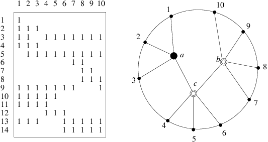
It follows that is represented by a bipartitive tree. For historical reasons, the prime nodes are known as C nodes, the degenerate nodes are known as P nodes and the bipartitive tree is called a PC tree [17, 28]. Figure 1 gives an example. When drawing a PC tree, we use the convention of representing a C node with a double circle and a P node with a dot. In this figure, the neighbor sets of are , , , , and . Each of these sets and the union of all but any one of these sets is a member of . For example, the neighbor set is a subset of rows , it contains rows , it does not strongly overlap row because the union of row 9 and is the entire column set, and it is disjoint from all other rows. Since it does not strongly overlap any row, it is a member of . Similarly, the union of all neighbor sets other than (the complement of ), is a member of . However, because is a C node (prime) the union of neighbor set and , which is neither the union of one neighbor set nor the union of all but one, is not a member of . This is verified by observing that it strongly overlaps row 12.
The neighbor sets of in the figure are , , , . Because it is a P node (degenerate), every union of at least one and fewer than all of these sets is a member of , and this is easily verified using similar checks.
Only unions of neighbor sets of a single internal node can be members of . For example, is not a union of neighbor sets of a single node, and it is not a member of because it strongly overlaps rows , , , , , and .
Note that has the circular-ones property, and the figure depicts a way to cyclically order the edges incident to each node such that in the resulting tree, every member of is consecutive in the circular ordering of leaves. This is an example of a general phenomenon:
Theorem 2.3 ([17]).
Let be the bipartitive tree for , where is the set family represented by rows of a circular-ones matrix with column set . Then:
- •
The edges incident to internal nodes can be cyclically ordered in such a way that the resulting cyclic order of leaves is a circular-ones ordering of the matrix;
- •
Reversing the cyclic order of edges about a prime node imposes a new circular-ones ordering on the leaves.
- •
Arbitrarily permuting the cyclic order of edges about a degenerate node imposes a new circular-ones ordering on the leaves.
- •
All circular-ones orderings of the leaves are obtainable by a sequence of these two operations.
This gives a convenient data structure, the PC tree, for representing all circular-ones orderings of a circular-ones matrix.
For example, in Figure 1, permuting the counterclockwise cyclic order of neighbors about so that it is and reversing the cyclic order of neighbors about so that it is imposes a new cyclic leaf order on the tree, , which is easily seen to be a circular-ones ordering.
To gain an insight into why this works, consider a circular-ones ordering of columns of a circular-ones matrix, let be a circularly consecutive set of columns, and let be the set represented by some row. If is removed and reinserted in reverse order, it will disrupt the consecutiveness of if and only if it strongly overlaps . Since is the family of sets that don’t strongly overlap any column, they are the sets that can be reversed in the cyclic order without disrupting the circular consecutiveness of any row. Each allowed rearrangement of the PC tree corresponds to a sequence of such reversals, and each such reversal is allowed by the PC tree.
The PC tree was first described by Shih and Hsu [28]. Its relationship to bipartitive set families and the circular-ones orderings of matrices was first described in [17].
It takes time linear in the size of a circular-ones matrix to build the PC tree even when a circular-ones ordering is not given as part of the input [17, 28]. As part of the output, a circular ordering of the edges incident to each internal node is given, which imposes a circular-ones ordering on the leaves. This gives a representation of all circular-ones orderings of the matrix in linear time.
Henceforth, we will assume for simplicity that every row of a circular-ones matrix has at least one 1 and one 0; any row without this property is irrelevant to the circular-ones arrangements.
3 Quotient labels for the PC tree
In this section, we give a way to label the nodes of the PC tree of a circular-ones matrix with quotients so that the matrix can be reconstructed from the labeling. These results were developed in [8], and the scheme is similar to ones developed for PQ trees in [20, 23, 25].
Recall that we assume that every row of the circular-ones matrix has at least one 1 and at least one 0, since a row that is all zeros or all ones has no effect on the circular-ones orderings of the matrix. Suppose that has a circular-ones ordering of columns. Consider the ordered tree that results from the PC tree of by the cyclic ordering about each node that is forced by the cyclic leaf order corresponding to the circular-ones ordering. For each row that has at least two 1’s we perform the following procedure. Root the PC tree at a leaf corresponding to a column with a 0 in . We maintain the order about each node in the following way. If is the counterclockwise order about and becomes the parent of , then becomes the linear order of children in the resulting ordered rooted tree. Let be the least common ancestor of the 1’s in . Let be the leaf descendants of a child of . Since , does not strongly overlap . Therefore, is either a subset of or disjoint from . It follows that consists of the leaf descendants of two or more children of . Moreover, since the cyclic order of edges about gives the circular-ones orderings of , consists of the neighbor sets of through a consecutive set of children of . Let be the projection of on . Figure 2 illustrates the concept.

As a special case, if has only one 1, let be the column where the 1 occurs, and let be its neighbor. We consider the projection of to be on , and to consist of ’s neighbor set .
When this projection has been performed on all rows, each internal node has received the projection of zero or more rows of , and we represent each projection with a row vector in a quotient matrix whose columns are neighbors of . The row has a 1 in column if the leaves reachable through are 1’s of and a 0 if they are 0’s in . The result is a matrix whose rows are sets of neighbors of . Note that the quotient at a node may be empty.
Figure 3 illustrates the quotients for the example of Figure 1. (The tree has been rooted at node ; the motivation for this is explained below.)

Lemma 3.1.
At a P node with neighbors, each row of the quotient matrix consists of either 1’s and one 0 or 0’s and one 1.
Proof.
Let be a circular-ones matrix, and let be the family of sets of columns obtained by considering each row to be the bit-vector representation of a set.
By the definition of a P node, every union of neighbor sets of is a member of . Let be the projection of some row to the quotient at . Suppose consists of more than one and fewer than neighbors of . Then consists of more than one and fewer than neighbor sets of . Let and be two neighbors of , one in and one not. Let and be the neighbor sets of reachable through and . Then is a union of neighbor sets of that strongly overlaps . This disqualifies it as a member of , contradicting the fact that every union of at least one and fewer than all neighbor sets of a P node is a member of . ∎
The quotient at node of Figure 3 illustrates the phenomenon. The projections of rows 2 and 4 exclude only neighbor , the projection of row 5 excludes only neighbor 1, the projection of row 3 excludes only neighbor 3, and the projection of row 1 contains only neighbor 1.
Lemma 3.2.
Any cyclic ordering of the quotient at a P node is a circular-ones ordering of it. The quotient at a C node has a unique circular-ones ordering, up to rotation and reversal.
Proof.
Again, let be a circular-ones matrix, and let be the family of sets of columns obtained by considering each row to be the bit-vector representation of a set.
The result follows immediately for P nodes by Lemma 3.1. Suppose is a Q node and let be the number of neighbors of . Let be an arbitrary union of more than one and fewer than neighbor sets of . By the definition of a Q node, . Therefore, it strongly overlaps some row of . Let be a column not in . Root the PC tree at . If projects to a proper descendant of , then is either a subset of or disjoint from , a contradiction to the strong overlap. If projects to a proper ancestor of , then , also a contradiction. If projects to a node that is neither an ancestor nor a descendant of , then is disjoint from , once again a contradiction. Therefore, projects on , and the projections and of and on are strongly overlapping sets of neighbors of .
We conclude that every set of more than one and fewer than neighbors of strongly overlaps some row of the quotient at . Reversing the order of members of in the cyclic ordering of neighbors about disrupts consecutiveness of . This implies that the PC tree of the quotient matrix at has a single internal node, a C node. The circular-ones orderings of this quotient are unique up to rotation and reversal. ∎
As an illustration, it is easily verified in Figure 3 that every ordering of columns of the quotients at P nodes is a circular-ones ordering, and that the quotient at C nodes and each have only two circular-ones orderings, one of which is depicted and the other of which is its cyclic reversal.
3.1 Computing the quotient-labeled PC tree in time linear in
Note that the linear-time PC-tree construction algorithm of [17] gives a circular-ones arrangement of the leaves, but does not label the nodes with their quotient. Let be the least common ancestor of a row when the tree is rooted at some leaf not in . Let a node be black if all of its leaf descendants are in . Because all neighbor sets of are either subsets of or disjoint from it, the black nodes consist of all ancestors of the leaves in , up to, and possibly including , if all of its children are black. The black children of are the ones corresponding to the projection of .
To find the projection of , we can therefore blacken the leaves that are members of . When we blacken a node we increment a counter in the parent, so that it keeps track of how many blackened children it has. When a node’s counter is incremented to a value that equals its number of children, we blacken it, and increment its parent’s counter. It is easily seen by induction on the height of a node that a node is blackened by this procedure if and only if it is black.
The procedure halts when no new vertex can be marked. The blackened nodes induce a rooted forest, which is a rooted tree if is black. Every internal node of this forest or tree has at least two black children. Therefore, the number of black internal nodes is bounded by the number of black leaves, which is the size of . Since the procedure spends time whenever it blackens a node, it takes time to find the least common ancestor and the edges to neighbor sets that make up ’s projection.
The procedure can be simulated without actually rooting the tree at ; it suffices to work “inward” from the marked leaves that are members of , and mark a node when its counter is equal to one less than its number of neighbors, since one of its neighbors is implicitly the parent. Since the entry in the quotient matrix has a 1 for each member of , it takes time to find the quotient representation of each row . The total time to find all quotients is therefore linear.
3.2 Computing the quotient-labeled PC tree in time
We now show that given a succinct representation of a circular-ones matrix, we may obtain the PC tree in time. By complementing a row of a binary matrix, we mean changing every 1 in the row to a 0 and every 0 to a 1. It is obvious that complementing a row of a circular-ones matrix yields a circular-ones matrix [13]. The following is given in [17] for the version of the PC tree where the nodes do not have quotient labels.
Lemma 3.3.
The PC tree of a circular-ones matrix is invariant under complementing a row of the matrix.
The lemma is obvious from the observation that does not change when a row is complemented.
Let be a column of a circular-ones matrix. Complementing all of the rows that have a 1 in column turns into a column of zeros. In the succinct representation of the matrix, it takes time to complement each such row: if represents the columns of the first and last 1 in the block of 1’s in the row, then the , modulo the number of columns, represents the complement of the row. Since now no row contains , a circular-ones ordering where is the last row of the matrix is a consecutive-ones ordering on the columns of the matrix, excluding .
The PQ tree was developed by Booth and Lueker to represent all consecutive-ones orderings of the columns of a consecutive-ones matrix [3]. It is a certain rooting of the PC tree. (The PC tree was originally developed to provide an easier way to compute the PQ tree. [28])
Lemma 3.4 ([17]).
Let be a circular-ones matrix and be a column. Let be the result of complementing all rows of that have a 1 in column , and then removing column . Removing leaf from the PC tree of and then rooting it at the neighbor of gives the PQ tree for .
Lemma 3.5.
It takes time to compute the PC tree of a circular-ones matrix, given a succinct representation of it.
Proof.
Given a succinct representation of a circular-ones matrix , we may remove all rows that have a single 1 or a single 0, since these have no effect on the circular-ones orderings of the matrix, hence on the PC tree. We may then select the last column of , and identify the rows with a 1 in column in time. We may complement each of them in time, as described above, for a total of time. We may remove from the resulting matrix by decrementing the record of the number of columns. This takes time and gives a succinct representation of a consecutive-ones matrix, .
In [26], an algorithm is given for finding the PQ tree of a consecutive-ones matrix, given a succinct representation. By Lemma 3.4 and the fact that the removed rows, which have all 0’s or all 1’s, have no effect on the PQ tree of , we may then add a new leaf corresponding to to the root of the tree produced by this algorithm, and then unroot it to obtain the PC tree of , also in time. ∎
Note that since the quotient labels of a PC tree have circular-ones orderings of columns, they can be expressed in the form of succinct representations also. Doing this for all quotient labels causes them to take space, since there is one quotient row for each row of the original matrix. This raises the question of whether we can find this succinct quotient-labeled PC tree in time.
Lemma 3.6.
Given a succinct representation of a circular-ones matrix with rows, it takes time to find the succinct quotient-labeled PC tree.
Proof.
The algorithm proceeds as in the proof of Lemma 3.5 until the PQ tree of the succinct representation of the consecutive-ones matrix has been computed. We install the succinct quotient labels in this PQ tree, as follows. We use Harel and Tarjan’s least-common ancestor algorithm [14] to find the least common ancestor of the endpoints of each interval, and the child that contains the right endpoint of each interval. Reversing the tree and repeating this gives the child containing the left endpoint. This takes time in total. These become the beginning and ending points for the representation of the row in the quotient at its least common ancestor.
For every row that was complemented to obtain from , we complement the image of the row in the quotient at its least common ancestor, which takes time for each of these rows. Note that if the image is all but one neighbor of a node and is not a leaf, then, after the complementation, this projection consists only of . However, the definition of the projection at the beginning of Section 3 dictates that in this case the projection be onto the least common ancestor of the row when the tree is rooted at a node that is 0 in the row. Now , not , is this node, so the the projection must be moved to , and be changed to consist of all neighbors of other than .
For each row that was removed because it has only one 1 or one 0, let be the leaf of the PC tree (column of the matrix) where the 1 or the 0 occurs. The projection is on the neighbor of , and consists either of or of all neighbors of other than , depending on whether the row had a 1 or a 0 in . ∎
4 Testing isomorphism of circular-ones matrices
In this section, we give an time algorithm, first developed in [8], to test isomorphism of two circular-ones matrices if no circular-ones ordering of the two matrices is given, and an algorithm if a succinct representation is given.
It is possible to test whether the matrices are both circular-ones matrices in linear time and to find a circular-ones ordering if they are [31]. If both of them fail to be circular-ones matrices, the input is rejected for failing to meet the precondition. If exactly one of them fails to be a circular-ones matrix, they are not isomorphic. Otherwise, from this ordering, we may find a succinct representation of the two matrices in linear time. We may then produce the quotient-labeled PC trees with a succinct representation of the quotients in time.
If the numbers of rows that are all 0’s in the two matrices differ or the number of rows of all ones differ, the matrices are not isomorphic. Otherwise, the problem reduces to the question of whether the two matrices are isomorphic when these rows are eliminated. Let and be these two matrices. This allows us to continue under our assumption that every row of the matrices has at least one 0 and at least one 1.
Let us define an isomorphism from one quotient-labeled PC tree, , to another one, to consist of the following. It must be that whenever and are nodes of , then and are adjacent in if and only if and are adjacent in . This is the standard notion of graph isomorphism. It must also satisfy an additional constraint. Each neighbor of internal node of corresponds to a column of the quotient matrix at . Each neighbor of node of is a column of the quotient matrix at . If is an isomorphism of the underlying trees, then let denote the bijection it induces from neighbors of to neighbors of . It must be the case that at each internal node , is an isomorphism from the quotient matrix at to the quotient matrix at . If such a exists, we say that the trees are isomorphic as quotient-labeled PC trees; otherwise we say that they are not. This definition precludes mapping a P node to a Q node, because the quotient label determines whether a node is a P node or a Q node.
Lemma 4.1.
Two circular-ones matrices are isomorphic if and only if their quotient-labeled PC trees are isomorphic.
Proof.
Suppose matrices and are circular-ones orderings of isomorphic circular-ones matrices. Let be an isomorphism from to . After permutation of columns of by , and have identical quotient-labeled PC trees, since they are identical multisets of row vectors. Since and are both circular-ones orderings of , is one of the permutations of columns of permitted by the quotient-labeled PC tree of . In other words, the PC tree of can be obtained from the PC tree of by the permitted operations. These operations define an isomorphism from the quotient-labeled PC tree of to the quotient-labeled PC tree of .
Conversely, suppose and are circular-ones orderings of matrices that have isomorphic quotient-labeled PC trees. Use the isomorphism to arrange the PC tree of so that it is identical to that of . Since it now represents instead of , it follows that the permutation of leaves of the PC tree induced by the isomorphism is an isomorphism from to . ∎
Lemma 4.1 is the basis of our algorithm: for two circular-ones matrices, we compute their quotient-labeled PC trees and test whether they are isomorphic. To test whether they are isomorphic, we encode the trees with strings in such a way that they both have the same encoding if and only if they are isomorphic.
4.1 Testing isomorphism of rooted, unordered trees
Our starting point is an algorithm for testing isomorphism of rooted, unordered trees that is given in the textbook [1]. A rooted tree is unordered if the left-to-right order of children of its nodes is not specified. Two unordered, rooted trees and are isomorphic if they are isomorphic as directed graphs when the edges are oriented from child to parent.
If the trees do not have the same height, they are not isomorphic. Otherwise, the algorithm proceeds by induction by level, from level 0, which is the level of the deepest leaf, to level , which is the level of the root and the height of the trees. At each level, it labels each node with an integer isomorphism-class label such that two nodes at the level have the same label if and only if the subtrees rooted at them are isomorphic. At step , we may assume by induction that this has been done for nodes at level . For all leaves at level , the isomorphism-class label is 0. For the remaining nodes, we may apply the following procedure. Let be the tuple of isomorphism-class labels for the children of , sorted in nondecreasing order. We may then sort the non-leaf nodes at level by lexicographic order of the tuples assigned to them, in order to group identical tuples together. If there are distinct tuples, among the tuples at level , we then assign isomorphism labels from 1 through to the tuples, and then each node with the number of the tuple it was assigned. By induction, this meets the precondition for induction step .
Therefore, two trees are isomorphic if their roots receive the same isomorphism class label.
4.2 Canonical encodings of quotients
An additional requirement of an isomorphism on quotient-labeled PC trees is that when a node of maps to a node in , then the neighbors of map to neighbors of in a way that is an isomorphism of the quotient at to the quotient at .
This requires that and have isomorphic quotients. In this subsection, we give an encoding of the quotient at a node of a quotient-labeled PC tree so that two nodes receive the same encoding if and only if their quotients are isomorphic.
4.2.1 P nodes
Consider the P node of Figure 3. An obstacle to an immediate canonical representation is that the quotient can be presented in any column order, since all column orders are circular-ones orderings.
By Lemma 3.1, every row of the quotient consists either of one of ’s neighbors, or of all but one of its neighbors. We can encode the quotient by giving, for each neighbor, an ordered pair of integers. The first integer is the number of rows that exclude only that neighbor and the second integer is number of rows that contain only that neighbor.
For example, at node in Figure 3, the tuple generated by neighbor 1 is , since the projection of one row, row 5, excludes only neighbor 1, and the projection of one row, row 1, contains only neighbor 1. The tuple generated at neighbor 2 is since no row contains only 2 and no row excludes only 2. The tuple generated at neighbor 3 is , since the projection of one row, row 3, excludes only neighbor 3 and no rows contain only neighbor 3. The tuple generated at neighbor is , since the projections of rows 2 and 4 exclude only and no row contains only . Note that the tuple generated at a neighbor is invariant under permutation of the cyclic order of neighbors about the P node.
Listing these tuples in the cyclic order of the nodes at which they are generated yields an encoding of the quotient. The next step of the construction is to sort the generated tuples lexicographically to obtain a tuple of tuples. In the example of node of Figure 3, this gives . This encoding is unique, since it is the lexicographic minimum of all tuples whose elements are the generated tuples.
Finally, in order to prevent the possibility that a P node and a C node will have the same encoding, we prepend a reserved P-node flag, 0, to the list of tuples. In the example if Figure 3, this gives .
This therefore gives a test of isomorphism of quotients at two P nodes by generating their canonical representations and testing whether they are equal.
4.2.2 A canonical encoding of the quotient at a C node
In generating a canonical encoding of the quotient at a C node , there are only two cyclic orders of the columns that are circular-ones orderings. One is the reverse of the other. This leaves us with two obstacles to a canonical representation: which of these two cyclic orders should we choose, and where in the cyclic ordering should we begin in developing a tuple to represent the quotient?
We begin by traveling counterclockwise around the cycle, starting at an arbitrary point. At each neighbor , we generate a tuple that lists the lengths of rows whose clockwise-most 1 is at , and list them in nondecreasing order.
For example, consider the C-node depicted in Figure 3. At neighbor , we see that there are two projections, of rows 11 and 10, whose clockwise endpoint is at , and they have lengths 2 and 3, respectively. Therefore, the tuple generated for neighbor is . At neighbor 4, there is one projection, of row 12, that has its clockwise endpoint at , and it has length 3, so the tuple generated for 4 is . Similarly, the tuples generated for neighbors 5, 6, and are , , and , respectively.
Assembling these tuples in clockwise order, we get . However, we must consider that we made an arbitrary decision in choosing the point on the circle at which to start generating the tuples. The effect of different choices is to rotate the resulting tuple of tuples. To choose it in a canonical way, we choose the rotation of the generated list of tuples that is earliest lexicographically: . We also made an arbitrary decision in going around the cycle clockwise instead of counterclockwise. Therefore, we repeat the above procedure counterclockwise, generating if starting at , and then choose the rotation of this that is lexicographically minimum, . To choose the direction of travel in a canonical way, we choose, from these two lists of tuples, the one that is earlier in lexicographic order: .
To avoid any possibility that a C node and a P node can get the same encoding, we prepend a reserved C-node flag, 1, to the list, yielding .
The general algorithm is as follows. First, we order the neighbors of the node so that the quotient has the circular-ones ordering. For each neighbor in counterclockwise order, list the lengths of the rows of the quotient whose clockwise-most 1 is at , in nondecreasing order. This gives a tuple for . The sequence of tuples generated for each neighbor , taken in counterclockwise order, gives a tuple of tuples. Rotate this ordering to get the lexicographic minimum through rotation of the tuples. Then repeat the exercise reversing the roles of clockwise and counterclockwise to obtain another such set of tuples. From these, select the one that is earlier lexicographically. Then prepend the reserved C-node flag 1 to this list.
If is an isomorphism, then the tuples generated at a neighbor of is the same as the one generated at neighbor of . Since the mapping of the cyclic ordering neighbors of to neighbors of is the cyclic ordering of neighbors of or its reverse, the quotient at and are encoded by the same tuple. Conversely, if the quotient at C nodes and have the same tuple, then since each tuple uniquely encodes cyclic rotations of the quotient, and have isomorphic quotients. Therefore, isomorphism of two quotients can be tested by determining whether they are encoded by the same quotient.
4.3 Testing isomorphism of quotient-labeled PC trees
We combine elements of the rooted-tree isomorphism test of Section 4.1 with the test for isomorphism of quotients of Section 4.2, in order to obtain an isomorphism test for quotient-labeled PC trees.
The use of elements of Section 4.1 requires us to root the PC trees. Conceptually, a rooting of a tree may be viewed as an orientation of its edges from child to parent, yielding a directed graph. An isomorphism from one rooted tree, , to another, , is a bijection from nodes of to nodes of such that for , is a directed edge in if and only if is a directed edge in . Once we root two PC trees, we require them to satisfy this condition. We must therefore be careful to root the two trees in an isomorphic way whenever they are isomorphic.
The center of a one-vertex tree is its vertex and the center of a one-edge tree is its edge. Otherwise, the center is obtained by deleting its leaves and recursively finding the center of the resulting subtree. It consists of a single vertex or a single edge.
If the center of a PC tree is node, we root it at that node. If it is an edge , we subdivide the edge with a pseudo-node and root it at so that the tree has a node as a root, as we did above. In the quotient at , replace the name of with and in the quotient at , replace the name of with . Now can be treated as a P node with an empty quotient.
Once we have rooted the trees, we proceed by induction on the level , as in the algorithm of Section 4.1. Because we are applying a stronger notion of isomorphism, which observes constraints imposed by the quotients, we must redefine what is meant by the isomorphism-class label assigned to a node at level .
For every node in we define a tree , an induced subtree of , as follows. If is a leaf node in , let be the one-node tree consisting of . If is an internal node that is not the root of , let be the quotient-labeled subtree induced by , its descendants, and the parent of . If is an internal node and the root of , then , and is the root of . Two nodes and at level are in the same isomorphism class at level if and only if and are isomorphic as quotient-labeled rooted PC trees.
Because of the inclusion of the parent of , the neighbors of each internal node of are the same in as they are in . This allows each internal node to retain the same quotient in as it has in . This tree is rooted at the parent of .
In order to merge the constraints of Sections 4.1 and 4.2, we prepend the isomorphism class label of a node at level (Section 4.1) to the tuple generated for the node in the encoding of the quotient (Section 4.2).
The preconditions at the beginning of the induction step at level are the following. Leaves at level are labeled with equivalence-class label 0. If is a non-leaf at level , then the parent of , if it exists, is a node of and labeled with equivalence class label -1. Note that is a leaf of , but no automorphism to itself will map to any other leaf of , since they are at different levels of . Therefore, we must give a different isomorphism class label from other leaves of .
For any other neighbor of , lies at level , and, by induction, it is labeled with an integer isomorphism class label for level . The isomorphism classes reflect the stronger constraints where, if and are two nodes at level that have the same label, and are isomorphic as rooted quotient-labeled PC trees. If, together in and , there are distinct isomorphism equivalence classes for internal nodes at level , they are labeled with integers between 1 and , where 1 denotes that a vertex is a leaf at level . For each neighbor of , let denote the integer label from assigned to .
We now strengthen the inductive step of Section 4.1 to make the stronger induction hypothesis go through for level . The canonical encoding of the quotient at given in Section 4.2 assigns a unique tuple to each neighbor of ; to this tuple we simply prepend to the tuple generated for . The labels on neighbors enforce the constraint that and can get the same tuple only if there is a bijection from neighbors of to neighbors of such that and are isomorphic as quotient-labeled trees. The rest of the tuple forces the constraint that they can get the same tuple only if there exists such a that is also an isomorphism from the quotient at to the quotient at , as in Section 4.2. Conversely, after ordering the tuples in the canonical way described in Section 4.2, it is clearly sufficient for and to be isomorphic as quotient-labeled trees for and to be assigned the same tuple.
Replacing the tuples with integer codes from 1 to , where is is the number of distinct tuples at level completes the induction step.
Therefore, and are isomorphic quotient-labeled PC trees if and only if, after rooting them at their centers and performing this algorithm, the roots get assigned the same integer label.
4.4 Time bound
Theorem 4.2.
Given the sparse representations of matrices and , it takes time either to determine that neither is a circular-ones matrix, or else to determine whether they are isomorphic. Given succinct representations of two circular-ones matrices, this problem takes time to solve.
Proof.
It takes time to determine whether they have the same number of 1’s, by counting 1’s in the two matrices in parallel. If so, . If the standard sparse representations of the matrices is given, it takes time to determine whether they are circular-ones matrices. If neither is, the claim is satisfied. If only one is, they are not isomorphic. Otherwise, it takes time to convert them to the succinct representations. From the succinct representations we can compute the two quotient-labeled PC trees, as described above.
Therefore, by Lemma 4.1, it suffices to show that the quotient-labeled PC-tree isomorphism algorithm can be implemented to run in time.
Proposition 1: Summing, for every level , the number of nodes at level plus the number of rows in quotients at level gives a number that is . This just counts the number of nodes in the tree plus the number of rows in the quotients. Each row of a matrix projects to just one row of a quotient.
Proposition 2: At level , the sum of lengths of the tuples is at most proportional to the number of nodes at level plus the number of rows in quotients at level . This is because one tuple is generated for each neighbor of contains an integer equivalence class label , and an encoding of a set of rows of the quotient at . The encoding of each row in the quotient only appears in one of the tuples for neighbors.
Proposition 3: At level , the maximum integer in any tuple is bounded by the number of nodes at level plus the number of rows in quotients at level . The integer equivalence classes at level are assigned consecutive numbers, starting at 2, by sorting the tuples lexicographically, and giving the same integer to two consecutive tuples that are identical, and giving an integer that is one higher than its predecessor’s if it differs from its predecessor. Each row of a quotient at level maps to only one element of a tuple generated at level .
Proposition 4: A radix sort of a set of tuples of integers takes time proportional to the sum of lengths of the tuples plus the size of the range of integer values occurring in the tuples [6].
The tuples at P nodes must be sorted lexicographically. Number the nodes at level in any order to assign them identification numbers, or I.D. numbers. The maximum number label of one of these nodes is at most the number of nodes at level . To each tuple for a child of a P node, prepend the I.D. number of the parent. Sort all tuples for P nodes at level in a single lexicographic sort. Since the I.D. number of the parent is the major sort key, this groups all tuples of children of a P node together, in lexicographic order, giving, for each P node, one lexicographically sorted list of tuples for its children. By Propositions 2, 3, and 4, the time for sorting all lists of tuples for children of P nodes conforms to the measure given in Proposition 1.
The order of tuples of children of a Q node are already given by the canonical procedure for generating them, as described above.
We must also sort the set of lists of tuples at level in order to generate the equivalence class numbers for the nodes at level . A list of tuples can be represented by a simple tuple of integers by appending a special separator, -2, to each tuple, and then concatenating them. This change of representation does not affect the lexicographic order of the lists, but turns them from lists of tuples to lists of integers to make it easier to see that they can be radix sorted. The addition of the separators increases the range of values by . By Propositions 2, 3, and 4, the time for sorting the set of lists of tuples for children of P nodes conforms to the measure given in Proposition 1.
Assigning integer equivalence-class labels to the lexicographically sorted set of lists of tuples trivially takes time proportional to the sum of lengths of lists of tuples, which, by Proposition 2, conforms to the measure of Proposition 1.
All of these steps conform to the measure of Proposition 1, so, by Proposition 1, they take time over all iterations of the induction step.
We must also bound the time to choose, from the possible choices of a list of tuples at a C node, one that is earliest in lexicographic order. Generate two lists, one for each cyclic ordering, starting at an arbitrary node for each. Turn each of the lists from a list of tuples to a list of integers, using the separators, as described above. Then apply the linear-time algorithm of [29] to find the cyclic rotation of each list that is earliest in lexicographic order. Of these two resulting lists, choose the one that is earlier in lexicographic order. ∎
5 Helly circular-arc graphs
Every interval model has the Helly property [10]. However, unlike interval models, circular-arc models may fail to have the Helly property. Figure 4 gives a circular-arc model of a graph where the arcs that make up a clique, , do not have a common intersection.
A graph is a Helly circular-arc graph if it admits at least one circular-arc model that has the Helly property. It is easily verified that there is no circular-arc model of the graph of Figure 4 where , , and have a common intersection point. This illustrates that the Helly circular-arc graphs are a proper subset of the circular-arc graphs.

Not every circular-arc model of a Helly circular-arc graph has the Helly property. Removing arcs from the model of Figure 4 yields a model for the complete graph on three vertices that does not have the Helly property. However, this graph is a Helly circular-arc graph; it is easy to represent this graph with three copies of the same arc, which has the Helly property.
The strategy of our algorithm for finding whether two Helly circular-arc graphs are isomorphic is related to that of Lueker and Booth for finding whether two interval graphs are isomorphic [23]; both algorithms use the clique matrices of the graphs. The main new challenge involves correctly computing the clique matrix.
We consider adjacency-list representations of two graphs and . Recall that we assume that the numbers of vertices and edges in both graphs are the same. For each graph, we obtain a Helly circular-arc model or determine that none exists, in time, using an existing algorithm for this problem [18]. If exactly one of them is a Helly circular-arc graph, we determine that they are non-isomorphic. If both of the input graphs fail to be Helly circular-arc graphs, we reject them for failing to meet the precondition, even though they may be isomorphic.
If both graphs are Helly circular-arc graphs, we use the Helly circular-arc models to find succinct representations of circular-ones orderings of their clique matrices. This involves some complications not present in the corresponding problem on interval graphs, which we show how to get around in time, below. Once we have succinct representations of the clique matrices, we use the straightforward fact that two graphs are isomorphic if and only if their clique matrices are isomorphic (Lemma 5.2, below). This reduces the problem to isomorphism of circular-ones matrices, which we have solved in time in Section 4.3. The total time is .
If the two graphs are circular-arc graphs and the inputs are circular-arc models, we use the algorithm of [18] to find a Helly circular-arc model for each of them or determine that it is not a Helly circular-arc graph. We then proceed as in the case where adjacency-list representations of two graphs are given, but take a total of time, rather than .
The main result of this section is the following theorem:
Theorem 5.1.
Given the adjacency-list representations of two graphs, and , where has vertices and edges, it takes time either to determine that neither is a Helly circular-arc graph, or else to determine whether they are isomorphic. Given circular-arc models of two circular-arc graphs, this problem takes time to solve.
If and are the number of vertices and edges of , it takes time to determine whether and , by counting these elements in the two graphs in parallel. If this is not the case, then they are not isomorphic. Therefore, we may assume henceforth that and .
Lemma 5.2 ([4]).
Two graphs are isomorphic if and only if their clique matrices are isomorphic.
Proof.
A graph isomorphism maps maximal cliques to maximal cliques, so it defines an isomorphism of their clique matrices. Conversely, since two vertices are adjacent if and only if they are in a common clique, an isomorphism from the clique matrix of one graph to that of another defines a graph isomorphism. ∎
In a circular-arc model of a graph, let an intersection segment be a place where a counterclockwise endpoint of an arc is followed immediately by a clockwise endpoint of an arc in the model in the clockwise direction; the intersection segment is the region between the two points. In an interval model, a set of arcs corresponds to a maximal clique if and only if it is the set of intervals containing an intersection segment. Each intersection segment can be located and marked by a clique point lying in the segment. A clique is a maximal clique if and only if it is the set of arcs that contain a clique point. A consecutive-ones ordering of the clique matrix can be obtained by making one column for each such maximal clique, and putting a 1 in the column in each row corresponding to an arc that passes through the region.
By analogy, in a Helly circular-arc model, we can place a clique point in each intersection segment. Because the model has the Helly property, a maximal clique must be the set of arcs containing one of the clique points. However, in contrast to the case of interval models, not all such sets of arcs must be maximal cliques. Moreover, the same clique may appear multiple times, as the arcs containing two different clique points in widely separated parts of the circle. Figure 5 gives an example.

To get a clique matrix for the graph, we must eliminate redundant clique points and clique points that do not represent maximal cliques from this Helly circular-arc model. Suppose we accomplish this. We can obtain a succinct representation of a circular-ones ordering of its clique matrix as follows. Number the arcs and label each arc’s two endpoints with its arc number. Create an array of buckets, one for each vertex. Number the cliques by numbering the clique points that have not been eliminated in order around the circle. This is a circular-ones ordering of the clique matrix.
It suffices, for each bucket , to store the counterclockwise-most and clockwise-most clique number of each arc in order to get the succinct representation of the circular-ones ordering of the clique matrix. The counterclockwise points that correspond to clique are those in the maximal consecutive block of counterclockwise points that lie immediately counterclockwise from clique point . The clockwise points that correspond to clique are those in the maximal consecutive block of clockwise endpoints immediately clockwise from clique point . This can be recorded in each bucket, giving the succinct representation of a circular-ones ordering of the clique matrix.
We now describe how to eliminate redundant clique points and clique points that do not correspond to maximal cliques. Since we have placed one clique point at each intersection segment, and each intersection segment contains the counterclockwise point of an arc and a clockwise point of an arc, we have placed at most clique points. A preliminary version of this procedure appeared in [21].
For any point on the circle of a circular-arc model, denote by the family of arcs of the model that contain . Given two points and on the circle of a circular-arc model, let us say dominates if . Let be a circular-arc model and be a set of points of the circle on which resides, where is the clockwise order in which appears in a traversal of the circle, starting at an arbitrary point on the circle. Let us say that is a -dominating set if every point in is dominated by some point in . Any minimal set of dominating points, with respect to containment, among the set of at most clique points we have placed on the circle, is a non-redundant set of clique points. We solve the following more general problem in time:
- •
Given a set of points on the circle of a (not necessarily Helly) circular-arc model, find a minimal -dominating set.
If the model is Helly and consists of one point per intersection segment, a minimal P-dominating set gives the columns of the clique matrix.
The ascending semi-dominating sequence of is the subset for all such that In other words, contains the points that are not dominated by any later point in . Similarly, the descending semi-dominating sequence of is the subset for all such that The following lemma reduces the problem of finding a minimal -dominating sequence to that of finding and .
Lemma 5.3.
Let be a circular-arc model and be a set of points on it. Both and are minimal -dominating sequences.
Proof.
We only prove that is a minimal -dominating sequence. The proof for can be obtained by taking the reverse of . Let be points on the circle where is the order in which appears in a clockwise traversal of the circle. We first prove that is in fact a -dominating sequence.
By definition, every point is dominated by some point for some . If is the minimum element in such that dominates , then no point can dominate ; otherwise would dominate , contradicting the minimality of . Therefore, every point in is dominated by some point in . We can apply a symmetric arguments for and to conclude that every point in is dominated by some point in . Since domination is a transitive relation, every point of is also dominated by some point in , i.e., is a -dominating sequence.
We now show that is minimal. Observe that it is enough to show that if a point is dominated by a point , where , then . This will imply that no point of dominates any other point of , so no point of can be removed from it to yield a smaller dominating set. If then , hence . If , then since , it follows that , and we obtain again that . ∎
The algorithms for finding and for finding are symmetric. We describe the one to find . The algorithm works by induction on to find , where . That is, we find those points of that are not dominated by any later points of .
By induction, assume we have the following partition of at the end of step :
- •
: points in that are already known to be in .
- •
: remaining points in ; these are points that are not dominated by any later point in , but that may or may not be dominated by points in .
It is easy to see that it will follow that when , we get that , and this solves the problem.
We begin with , where and .
In step , we obtain and from and as follows. We remove points from and insert them in if they pass a test that shows that they cannot be dominated by any later point in , including . The addition of these points to gives . We discard other points from that are dominated by . We then add to . This gives .
The test of whether a point moves from to consists of determining whether it is contained in the arc that does not contain , has its clockwise endpoint in , and among all such arcs, extends farthest in the counterclockwise direction. (See Figure 6.) If is contained in , then, since does not contain any point from , cannot be dominated by any point in this set, and since , it it is not dominated by any later point in . Therefore, it is a member of , and can be moved to .

We implement as a stack , where is the top of the stack. Note that the set of points that get moved to are consecutive at the top of the stack. To move them, we pop the stack until we reach an element not in , and move the popped elements to .
A point that is still in fails to be dominated by if and only if it is contained in some arc that does not contain . All arcs in this set contain , since otherwise, would already be identified as a member of for some .
Of all arcs that exclude but contain , let be the one whose clockwise endpoint extends farthest clockwise from . (See Figure 6.) Since is the arc in this set that covers the most members of , it follows that the points of that are dominated by are those that are not contained in .
Note that the ones that are dominated by are again consecutive at the top of the stack, so we pop the stack until we reach an element that is contained in , and discard the popped elements.
Since belongs in , we obtain our stack for by pushing to what remains of the stack for .
For the time bound, note that we may find for each by traversing comparing the counterclockwise endpoints of arcs whose clockwise endpoints are in this interval and do not contain . Over all , this expends time on each arc, so it takes time.
To find for all , we start just counterclockwise from and traverse the circle counterclockwise, keeping track of the best arc so far. The best arc is initially null. When we reach an arc , we check whether contains , and, if so, whether it extends farther clockwise than the best arc so far. If so, becomes the best arc so far. Each time we reach a point , we record the best arc so far as . Over all , this also expends time on each arc, for a total of time.
The management of the stack implementing takes time over all steps, since each point is pushed once, and when points are popped, they are consecutive at the top of the stack.
6 Isomorphism of circular-arc graphs, convex-round graphs, and proper circular-arc graphs
In this section we show that the circular-ones matrix isomorphism test of Section 4 can be used to test isomorphism of circular-arc graphs and convex-round graphs, using results of Chen [5]. From this we get a new algorithm for isomorphism of proper circular-arc graphs.
Theorem 6.1.
Given adjacency lists of two graphs, it takes time to either determine that the graph are not circular-arc graphs or to determine whether they are isomorphic.
Theorem 6.2.
Given adjacency lists of two graphs, it takes time to either determine that the graph are not convex-round graphs or to determine whether they are isomorphic.
A graph is a circular-arc graphs if its augmented adjacency matrix has the circular-ones property. Chen [5] showed that two circular-arc graphs are isomorphic if and only if their augmented adjacency matrices are isomorphic.
Given adjacency-list representations of two graphs, it takes time to determine whether their augmented adjacency matrices have the circular-ones property [13, 17, 31]. If they both do, then it takes time, using the isomorphism test of Section 4 to determine whether they are isomorphic. If a circular-one ordering of the adjacency matrices of the two graphs are given using succinct representations, the test takes time.
Convex-round graphs are complements of circular-arc graphs [2]. The adjacency matrix of a convex-round graph has the circular-ones property. Chen [5] showed that two convex-round graph are isomorphic if and only if their adjacency matrices are isomorphic. Therefore, we use the same technique to get the same bounds for testing isomorphism of convex-round graphs as we do for testing isomorphism of circular-arc graphs.
Since every proper circular-arc graph is a circular-arc graph [31], we can use the same algorithm also for an isomorphism test of proper circular-arc graphs. This gives a new isomorphism algorithm for proper circular-arc graph.
The time bound is optimal if the input graphs are given by adjacency lists, but it is not optimal if they are given by proper circular-arc models. The algorithm of Lin et al. [22] for the problem solves it in time if the circular-arc models are given. We show how to achieve an algorithm with the same time bound. We need to find succinct representations of circular-one arrangements of the augmented adjacency matrix of the given proper circular-arc models.
Let be a circular-arc model of . If is not a proper circular-arc model, then we can convert it in time to such a model [27]. The model can be changed in time, such that no two arcs cover the circle together [19, 24], and the model remains proper. After changing the model this way, we index the vertices of according to the clockwise order of their counterclockwise endpoints, starting at an arbitrary endpoint. Since there are no arc containment or pair of arcs that cover the circle in , this indexing gives a circular-ones arrangement of the augmented adjacency matrix of .
To find the last 1 entry in the row of each vertex of according to this indexing, in time, we go clockwise around the circle once, starting at an arbitrary counterclockwise endpoint, which belongs to a vertex . If the next endpoint we encounter is a clockwise endpoint of a vertex , then the last 1 in the row of is in the column of . If the next endpoint we encounter is a counterclockwise endpoint of a vertex , we set . We end this traversal when we get back to the start point. The first 1 of every row of a vertex in is found symmetrically.
We conclude that it takes time to find a succinct representation of a circular-ones ordering of the augmented adjacency matrix of a graph from a proper circular-arc model of the same graph. Once we have succinct representation of the augmented adjacency matrices of and we can test them for isomorphism in time.
Theorem 6.3.
Given adjacency lists of two graphs, it takes time to either determine that the graph are not proper circular-arc graphs or to determine whether they are isomorphic. Given two circular-arc models of circular-arc graphs, the same task takes time.
7 Hsu’s algorithm for circular-arc graphs isomorphism
In this section we give an example of two circular-arc graphs that are not isomorphic, but the algorithm of Hsu [15] determines that they are. We begin with few definitions from this paper. Let be a circular-arc graph, without universal vertices, and without any pair of vertices and such that . A normalized model of is a circular-arc model of the graph, such that for every two arcs and : (1) if then the arc of contains the arc of ; (2) if every satisfies and every satisfies then the arcs of and cover the circle together. Every circular graph without universal arcs and without any pair of vertices with the same neighborhood has a normalized model [15].
Let be a normalized model of . We get the associated chord model of by replacing the arcs of with chords. Let be an associated chord model of . The chord model represents a circle graph , whose vertex set is the same vertex set as of , and two vertices are adjacent if and only if their chords in intersect. Although there might be more than one unique associated chord model for , the graph is unique. Hsu [15] defined a type of chord model called conformal model for . The chord model is a conformal model of . Note that we do not repeat the definition of conformal model here, we just give an example for one such model. We do not require the definition for our purposes.
The origin of the mistake in Hsu’s algorithm is the statement “To test the isomorphism between two such circular-arc graphs and , it suffices to test whether there exist isomorphic conformal models for and ” [15, Section 9], where “such circular-arc graphs” refer to circular-arc graphs for which both and its complement are connected.
Consider the graphs and in Figure 7. It is easy to see that and are not isomorphic, since they have different number of edges. Normalized circular-arc models of both graphs are given in Figure 8. From the circular-arc models, we can see that the chord model in Figure 9 is an associated chord model for both graphs, and hence a conformal model of both and . The graphs are connected and so are their complements. We conclude that the statement above is wrong, and the algorithm of [15] falsely finds that and are isomorphic.


Hsu [16] noted that the isomorphism of conformal models of and , which the algorithm of [15] produces, does give a mapping between vertices of and , if is inseparable with respect to modular decomposition. However, we do not know how to handle the case when this condition is not satisfied. We note that the algorithm of [15] works correctly for isomorphism of circle graphs. With the time recognition algorithm for circle graphs [30], the isomorphism test takes time if the graphs are given as adjacency matrices. The recent circle-graph recognition algorithm [12] leads to the same running time for circle-graph isomorphism, where is the inverse Ackermann function. If chord models are given as an input, then the running time of the isomorphism test can be reduced to using techniques similar to those used in [22] and in our paper.
References
- [1] A. V. Aho, J. E. Hopcroft, and J. D. Ullman. The Design and Analysis of Computer Algorithms. Addison-Wesley, Reading, Massachusetts, 1974.
- [2] J. Bang-Jensen, J. Huang, and A. Yeo. Convex-round and concave-round graphs. SIAM J. Discrete Math., 13:179–193, 2000.
- [3] S. Booth and S. Lueker. Testing for the consecutive ones property, interval graphs, and graph planarity using PQ-tree algorithms. J. Comput. Syst. Sci., 13:335–379, 1976.
- [4] L. Chen. Graph isomorphism and identification matrices: Parallel algorithms. IEEE Trans. Parallel Distrib. Syst., 7(3):308–319, 1996.
- [5] L. Chen. A selected tour of the theory of identification matrices. Theor. Comput. Sci., 240:299–318, 2000.
- [6] T. H. Cormen, C. E. Leiserson, R. L. Rivest, and C. Stein. Introduction to Algorithms. McGraw Hill, Boston, 2001.
- [7] W. H. Cunningham and J. Edmonds. A combinatorial decomposition theory. Canadian J. Math., 32:734–765, 1980.
- [8] A. R. Curtis. Linear-time graph algorithms for chordal comparability graphs and helly circular arc graphs. Master’s thesis, Colorado State University, 2007.
- [9] E. M. Eschen. Circular-arc graph recognition and related problems. PhD thesis, Department of Computer Science, Vanderbilt University, 1997.
- [10] D. R. Fulkerson and O. Gross. Incidence matrices and interval graphs. Pacific J. Math., 15:835–855, 1965.
- [11] F. Gavril. Algorithms on circular-arc graphs. Networks, 4:357–369, 1974.
- [12] E. Gioan, C. Paul, M. Tedder, and D. G. Corneil. Circle graph recognition in time . arXiv:1104.3284v2 [cs.DS], 2011.
- [13] M. C. Golumbic. Algorithmic Graph Theory and Perfect Graphs. Academic Press, New York, 1980.
- [14] D. Harel and R. E. Tarjan. Fast algorithms for finding nearest common ancestors. SIAM J. Comput., 13:338–355, 1984.
- [15] W. L. Hsu. algorithms for the recognition and isomorphism problems on circular-arc graphs. SIAM J. Comput., 24:411–439, 1995.
- [16] W. L. Hsu. Personal communication, 2008.
- [17] W. L. Hsu and R. M. McConnell. PC trees and circular-ones arrangements. Theor. Comput. Sci., 296:59–74, 2003.
- [18] B. L. Joeris, M. C. Lin, R. M. McConnell, J. P. Spinrad, and J. L. Szwarcfiter. Linear-time recognition of helly circular-arc models and graphs. Algorithmica, 59:215–239, 2011.
- [19] H. Kaplan and Y. Nussbaum. Certifying algorithms for recognizing proper circular-arc graphs and unit circular-arc graphs. Discret. Appl. Math., 157:3216–3230, 2009.
- [20] N. Korte and R. H. Möhring. An incremental linear-time algorithm for recognizing interval graphs. SIAM J. Comput., 18:68–81, 1989.
- [21] M. Lin, R. M. McConnell, F. J. Soulignac, and J. L. Szwarcfiter. On cliques of helly circular-arc graphs. The IV Latin-American Algorithms, Graphs, and Optimization Symposium, Electronic Notes in Discrete Mathematics, 30:117–122, 2008.
- [22] M. Lin, F. J. Soulignac, and J. L. Szwarcfiter. A simple linear time algorithm for the isomorphism problem on proper circular-arc graphs. SWAT 2008, 11th Scandinavian Workshop on Algorithm Theory, Lecture Notes in Computer Science, 5124:355–366, 2008.
- [23] G. S. Lueker and K. S. Booth. A linear time algorithm for deciding interval graph isomorphism. J. ACM, 26:183–195, 1979.
- [24] Lin M. and Szwarcfiter J. L. Unit circular-arc graph representations and feasible circulations. SIAM J. Discret. Math., 22:409–423, 2008.
- [25] R. M. McConnell. A certifying algorithm for the consecutive-ones property. Proceedings of the 15th Annual ACM-SIAM Symposium on Discrete Algorithms (SODA ’04), 15:761–770, 2004.
- [26] R. M. McConnell and F. de Montgolfier. Algebraic operations on PQ trees and modular decomposition trees. Proceedings of the 31st Workshop on Graph Theoretic Concepts in Computer Science (WG ’05), Lecture Nodes in Computer Science, 3787:421–432, 2005.
- [27] Y. Nussbaum. From a circular-arc model to a proper circular-arc model. Proceedings of the 34th Workshop on Graph Theoretic Concepts in Computer Science (WG ’08), Lecture Nodes in Computer Science, 5344:324–335, 2008.
- [28] W. K. Shih and W. K. Hsu. A new planarity test. Theor. Comput. Sci., 223:179–191, 1999.
- [29] Y. Shiloach. Fast canonization of circular strings. J. Algorithms, 2:107–121, 1981.
- [30] J. Spinrad. Recognition of circle graphs. J. Algorithms, 16:264–282, 1994.
- [31] A. Tucker. Matrix characterizations of circular-arc graphs. Pacific J. Math, 39:535–545, 1971.
- [32] T. H. Wu. An isomorphism test for circular-arc graphs. PhD thesis, Applied Mathematics and Statistics, SUNY-Stonybrook, 1983.