Dynamical equilibration of strongly interacting “infinite” parton matter within the Parton-Hadron-String Dynamics (PHSD) transport approach
Abstract
We study the kinetic and chemical equilibration in “infinite” parton matter within the parton-hadron-string dynamics off-shell transport approach, which is based on a dynamical quasiparticle model (DQPM) for partons matched to reproduce lattice QCD results—including the partonic equation of state—in thermodynamic equilibrium. The “infinite” parton matter is simulated by a system of quarks and gluons within a cubic box with periodic boundary conditions, at various energy densities, initialized out of kinetic and chemical equilibrium. We investigate the approach of the system to equilibrium and the time scales for the equilibration of different observables. We, furthermore, study particle distributions in the strongly interacting quark-gluon plasma (sQGP) including partonic spectral functions, momentum distributions, abundances of the different parton species, and their fluctuations (scaled variance, skewness, and kurtosis) in equilibrium. We also compare the results of the microscopic calculations with the ansatz of the DQPM. It is found that the results of the transport calculations are in equilibrium well matched by the DQPM for quarks and antiquarks, while the gluon spectral function shows a slightly different shape due to the mass dependence of the gluon width generated by the explicit interactions of partons. The time scales for the relaxation of fluctuation observables are found to be shorter than those for the average values. Furthermore, in the local subsystem, a strong change of the fluctuation observables with the size of the local volume is observed. These fluctuations no longer correspond to those of the full system and are reduced to Poissonian distributions when the volume of the local subsystem becomes small.
I Introduction
Nucleus-nucleus collisions at ultrarelativistic energies are studied experimentally and theoretically to obtain information about the properties of hadrons at high density and/or temperature as well as about the phase transition to a new state of matter, the quark-gluon plasma (QGP). Whereas the early “big bang” of the universe most likely evolved through steps of kinetic and chemical equilibrium, the laboratory “tiny bangs” proceed through phase-space configurations that initially are far from an equilibrium phase and then evolve by fast expansion. On the other hand, many observables from strongly interacting systems are dominated by many-body phase space such that spectra and abundances look “thermal.” It is thus tempting to characterize the experimental observables by global thermodynamical quantities such as “temperature,” chemical potentials or entropy [1, 2, 3, 4, 5, 6, 7, 8]. We note that the use of macroscopic models such as hydrodynamics [9, 10, 11, 12] employs as a basic assumption the concept of local thermal and chemical equilibrium in the infinite-volume limit, although by introducing different chemical potentials one may treat chemical off-equilibrium also in hydrodynamics. The crucial question, however, of how and on what time scales thermodynamic equilibrium can be achieved is presently a matter of debate. Thus nonequilibrium approaches have been used in the past to address the problem of time scales associated with global or local equilibration [13, 14, 15, 16, 17, 18, 19, 20]. Another question is the influence of finite-size effects on fluctuation observables and the possibility of relating experimental observations in relativistic heavy-ion collisions to the theoretical predictions obtained in the thermodynamic limit. Therefore, a thorough microscopic study of the questions of thermalization and equilibration of confined and deconfined matter within a nonequilibrium transport approach, incorporating both hadronic and partonic degrees of freedom and the dynamic phase transition, appears timely.
The paper is organized as follows. In Sec. II we provide a brief reminder of the off-shell dynamics and the ingredients of the transport approach. We then present in Sec. III the actual results on the chemical equilibration of the partonic matter in parton-hadron-string dynamics (PHSD). In Sec. IV we investigate the properties of the partonic matter in chemical and kinetic equilibrium and compare the particle properties in equilibrium with the dynamical quasiparticle model (DQPM), which has been developed to describe the thermodynamics of lattice QCD. In Sec. V we study (within the dynamical approach) the parton properties at finite quark chemical potential , while in Sec. VI higher moments of parton distributions and the equilibration of fluctuation observables as well as the size of fluctuations in equilibrium are investigated. We then show in Sec. VII the time scales for the relaxation of fluctuation observables in comparison to the time scales for the equilibration of the average values of the observables. Finally, a summary and conclusions are given in Sec. VIII.
II The Parton-Hadron-String Dynamics transport approach
In this work we study the kinetic and chemical equilibration in “infinite” parton matter within the Parton-Hadron-String Dynamics (PHSD) transport approach [21, 22], which is based on generalized transport equations on the basis of the off-shell Kadanoff-Baym equations [23, 24] for Green’s functions in phase-space representation (in the first order gradient expansion, beyond the quasiparticle approximation). The approach consistently describes the full evolution of a relativistic heavy-ion collision from the initial hard scatterings and string formation through the dynamical deconfinement phase transition to the strongly interacting quark-gluon plasma (sQGP) as well as hadronization and the subsequent interactions in the expanding hadronic phase. In the hadronic sector PHSD is equivalent to the Hadron-String-Dynamics (HSD) transport approach [25, 26] that has been used for the description of and collisions from GSI heavy ion synchrotron (SIS) to Relativistic Heavy Ion Collider (RHIC) energies in the past.
In particular, PHSD incorporates off-shell dynamics for partons and hadrons. In the off-shell transport description, the hadron and parton spectral functions change dynamically during the propagation through the medium and—in case of hadrons—evolve toward the on-shell spectral function in vacuum if the system expands in the course of the heavy-ion collisions. As demonstrated in [27, 28] the off-shell dynamics is important for hadronic resonances with a rather long lifetime in vacuum but strongly decreasing lifetime in the nuclear medium (especially and mesons) and also proves vital for the correct description of dilepton decays of mesons with masses close to the two-pion decay threshold.
II.1 Off-shell transport
Let us recall the off-shell transport equations (see [29] for details). One starts with a first-order gradient expansion of the Wigner-transformed Kadanoff-Baym equation and arrives at the generalized transport equation [27, 23]
| (1) |
where the curly brackets denote the relativistic generalization of the Poisson bracket
One additionally obtains a generalized mass-shell equation
| (2) |
with the mass function . In Eqs. (1) and (2) the Green’s functions stand for the expectation values of the quantum fields (denoted here by ),
| (3) |
with for bosons and for fermions, while the self-energies are given by the functional derivative of with respect to the full propagator :
| (4) |
In (4) the functional is the sum of all closed two-particle-irreducible (2PI) diagrams built up by full propagators .
The retarded and advanced Green’s functions and are given as
| (5) | |||
| (6) |
These Green’s functions contain exclusively spectral but no statistical information of the system. Their time evolution is determined by Dyson-Schwinger equations (cf. Ref. [27]). Retarded and advanced self-energies and are defined in analogy to Eqs. (5) and (6).
In the transport equation (1) one recognizes on the left-hand side the drift term , as well as the Vlasov term with the real part of the retarded self-energy . On the other hand the right-hand side represents the collision term with its typical “gain and loss” structure. Thus interaction between the degrees of freedom is thus incorporated into the mean fields and collisions as in the Vlasov-Boltzmann “standard” transport approach [30]. In contrast, in the off-shell transport there is an additional term , which is denoted as the back-flow term and is responsible for the proper off-shell propagation. It vanishes in the on-shell quasiparticle limit. Note, however, that the self-energies fully determine the dynamics of the Green’s functions for given initial conditions.
We, further on, represent Eqs. (1) and (2) in terms of real quantities by the decomposition of the retarded and advanced Green’s functions and self-energies as
| (7) | |||
| (8) |
| (9) | |||
| (10) |
We note that in Wigner space the real parts of the retarded and advanced Green’s functions and self-energies are equal, while the imaginary parts have opposite sign and are proportional to the spectral function and to the width , respectively.
With the redefinitions (7)–(10) one obtains two algebraic relations for the spectral function and the real part of the retarded Green’s function, , in terms of the width and the real part of the retarded self-energy, , as [27, 29]
| (11) | |||
| (12) |
Note that all terms with first-order gradients have disappeared in (11) and (12). A first consequence of (12) is a direct relation between the real and the imaginary parts of the retarded, advanced Green’s function, which reads (for )
| (13) |
Inserting (13) in (11) we end up with the following result for the spectral function and the real part of the retarded Green’s function:
| (14) | |||
| (15) |
The spectral function (14) shows a typical Breit-Wigner shape with energy- and momentum-dependent self-energy terms. Although the above equations are purely algebraic solutions and contain no derivative terms, they are valid up to the first order in the gradients.
In addition, subtraction of the real parts and adding up the imaginary parts lead to the time evolution equations
| (16) | |||
| (17) |
When inserting (14) and (15) we find that these first-order time-evolution equations are solved by the algebraic expressions. Accordingly, the time evolution of the system is fully defined by and the width in (1).
We recall that the off-shell transport equation (1) can be solved explicitly by employing a generalized test-particle ansatz for the real quantity . For the explicit equations of motion for these test particles we refer the reader to Ref. [29].
II.2 Explicit equations for fermions
In case of fermions—such as baryons or quarks—the self-energy is separated into different Lorentz structures of scalar and vector type:
| (18) |
for each fermion species . The mass function for fermions is then
| (19) |
with the effective mass and four-momentum given by
| (20) | |||
| (21) |
where stands for the bare (vacuum) mass. After inserting (19) into the generalized transport equation (1), the covariant off-shell transport theory emerges. It is formally written as a coupled set of transport equations for the phase-space distributions of fermion with a spectral function [using ], i.e.,
| (22) | |||||
with
and
Here and . The factor stands for the in-medium transition matrix element (squared) for the binary reaction , which has to be known also off the mass shell. The back-flow term in (22) is given by
As pointed out before this expression stands for the off-shell evolution, which vanishes in the on-shell limit or when the spectral function does not change its shape during the propagation through the medium, i.e., for and . We recall that the transport equation (22) has been the basis for the off-shell HSD transport approach for the baryon and antibaryon dynamics.
II.3 The dynamical quasiparticle model
The basis of the partonic phase description is the dynamical quasiparticle model [31, 32], which has been matched to reproduce lattice QCD results (lQCD)—including the partonic equation of state—in thermodynamic equilibrium. The DQPM allows for a simple and transparent interpretation of thermodynamic quantities as well as correlators—measured on the lattice—by means of effective strongly interacting partonic quasiparticles with broad spectral functions. The essential quantities in the DQPM are “resummed” single-particle propagators , , and . We stress that a nonvanishing width in the partonic spectral function is the main difference between the DQPM and conventional quasiparticle models [33]. Its influence on the collision dynamics is essentially seen in the correlation functions; e.g., in the stationary limit, the correlation involving the off-diagonal elements of the energy-momentum tensor define the shear viscosity of the medium [34]. Here a sizable width is mandatory to obtain a small ratio of the shear viscosity to entropy density, [35], which results in a roughly hydrodynamical evolution of the partonic system in PHSD [22]. The finite width leads to two-particle correlations, which are taken into account in PHSD by means of the generalized off-shell transport equations (cf. Sec. II.A) that go beyond the mean-field or Boltzmann approximations.
In the scope of the DQPM the running coupling constant (squared) for is approximated by
| (24) |
where the parameters and have been extracted from a fit to the lattice QCD equation of state as described in Refs. [36, 40]. In (24), stands for the number of colors, is the critical temperature (= MeV), while (=3) denotes the number of flavors.
In the asymptotic high-momentum (high-temperature) regime, the functional form of the parton quasiparticle mass is chosen to coincide with that of the perturbative thermal mass, i.e., for gluons
| (25) |
and for quarks (antiquarks)
| (26) |
but with the coupling given in (24). The effective quarks, antiquarks, and gluons in the DQPM have finite widths, which for are approximated by
| (27) | |||||
| (28) |
where (from Refs. [34]) is related to a magnetic cutoff. Note that for the DQPM gives
| (29) |
From the expressions (24)–(29), one can see that at high temperature, , the masses and the interaction strength of the quasiparticles in the DQPM are approaching the one-loop perturbative QCD results. However, the one-loop functional form is not the relevant description at temperatures close to or even below. The transition region (approximately ) is dominated by nonperturbative phenomena. Therefore, we implement in PHSD for the transitional values of (the region ) functional forms for and , which are growing softer with decreasing as compared to the perturbative logarithmic divergence in (24). The actual values of and have been shown as functions of temperature as well as the scalar parton density in Ref. [40]. A comparison to the lQCD interaction measure [39] has been presented also in Ref. [40] (cf. Figs. 1, 2, and 4).
We note in passing that the smooth parametrizations for and at close to nicely reproduce the recent lQCD calculations from the Wuppertal-Budapest group [39]. As a consequence, we obtain not only a quantitatively good description of the phase transition region but also a smooth “interpolation” from the hadron-dominated systems to those with dominant partonic degrees of freedom.
With the parton masses and widths fixed by (24)–(29) the spectral functions can be written [in alternative form to (14)] as
| (30) | |||||
separately for quarks, antiquarks, and gluons (), with the notation . We may identify (cf. Sec. II.A)
| (31) |
The spectral function (30) is antisymmetric in and normalized as
| (32) |
The parameters and from the DQPM have been defined above in the Eqs. (25)–(29). Note that the DQPM assumes ; we will discuss the consequences of this approximation in Sec. IV. Also, the decomposition of the total width into the collisional width (due to elastic and inelastic collisions) and the decay width is not addressed in the DQPM. Therefore, we dedicate the next section to this question and to a brief description of the microscopic implementation of the deconfined phase of QCD within the PHSD.
II.4 Reaction rates and effective cross sections
In this section we present the effective cross sections for each of the various partonic channels as a function of energy density ; these cross sections determine the partial widths of the dynamical quasiparticles as well as the various interaction rates. This analysis is important, because, although the DQPM provides the basis of the description of the strongly interacting quark-gluon system in PHSD in equilibrium, the dynamical transport approach (i.e., PHSD) goes beyond the DQPM in simulating hadronic and partonic systems also out of equilibrium. For the microscopic transport calculations, the partial widths of the microscopic scattering and decay channels have to be known, while the DQPM provides only the total widths of the dynamical quasiparticles that have been fixed by lattice QCD calculations as described in Sec. II.C and in more detail in Refs. [31, 32]. Furthermore, the explicit shape of the partonic spectral functions—taken as Lorentzians in the DQPM (30)—will depend on the decomposition of the interaction into particular channels within the coupled-channel dynamics of PHSD.
In order to fix the partial cross sections for the interactions between the dynamical quarks and gluons (as functions of energy density ) we perform PHSD calculations in a cubic finite box with periodic boundary conditions—simulating “infinite” hadronic or partonic matter. In this particular case the derivatives of the retarded self-energies with respect to space vanish in (22) such that we essentially deal with the parton dynamics due to the collision terms in (22).
The following (quasi)elastic interactions among quarks, antiquarks, and gluons () are implemented in PHSD:
| (33) | |||||
| (34) | |||||
| (35) | |||||
| (36) | |||||
| (37) | |||||
| (38) |
The (quasi)elastic processes (33)–(38) play a crucial role for the thermalization in PHSD due to the possibility to change the masses of interacting partons in the final state as shown in Eq. (33).
The flavor exchange of partons is possible only within the inelastic interactions in PHSD, which are:
| (39) | |||||
| (40) | |||||
| (41) |
The inelastic interactions (39)–(41) are the basic processes for the chemical equilibration in PHSD; however, the inelastic processes [(40 and (41)] are strongly suppressed () kinematically in PHSD due to the large masses of gluons.
We recall that for binary channels we have explicit formulas for the partial widths, e.g. [from the collision term in (22)],
| (42) |
where is an index, which can be equal to “”, “” or “,” where . Since we study partons at high temperature the fermion blocking terms can be neglected, i.e., approximated by , and one ends up with
| (43) |
where the four-momenta of particle 4 are fixed by energy-momentum conservation and stands for the two-body phase-space integral (cf. [41]). We recall that the squared matrix element times the two-body phase-space integral defines a binary cross section times a kinematic factor, i.e.,
| (44) |
with the relativistic relative velocity for initial invariant energy squared, , given by
| (45) |
In (44) stands for a summation over discrete final channels.
If the cross section is essentially independent of the momenta, which should hold for low-energy binary scattering, we may write (43) as
| (46) |
which corresponds to the Boltzmann limit relating the collision rate to the average velocity between the colliding partners (in the center-of-mass frame) and the cross section for scattering as well as the density (summed over the discrete quantum numbers of particle 2). We employ these relations in determining the effective elastic cross sections between partons in the PHSD. Note that the total number of collisions between particles of type 1 and 2 are obtained from (46) (in our case) by multiplication with the volume and the particle density , i.e.,
| (47) |
Both the number of collisions between the individual particle species as well as their densities are easily accessible in the transport approach.

The cross section for gluon formation from flavor-neutral interactions in the color octet channel is calculated by the resonant cross section at invariant energy squared, ,
| (48) |
with
| (49) |
while the factor 2/4 corresponds to the ratio of final to initial spins (assuming two transverse degrees of freedom for the gluon in line with the DQPM). Note that formula (48) provides an off-shell cross section which depends on the four-momenta of the incoming quark and antiquark as well as on the spectral properties of the gluon. We recall that in the actual simulation the quark and antiquark masses are distributed according to the spectral function (30) and their three-momenta vary in a broad range roughly in line with thermal Boltzmann distributions.
We point out that the iteration of the coupled equations has been performed with the additional boundary conditions
| (50) |
as suggested by lattice QCD, which roughly follows a scaling with the color Casimir operators. This is also reflected in the DQPM ansatz (29). We mention that this scaling might be violated and require a further independent parameter, which, however, presently cannot be fixed appropriately by lQCD calculations. The function has to be determined by the iteration procedure until self-consistency has been reached for each value of energy density . Note that for = 0 we have identical phase-space distributions for quarks and antiquarks and also identical interaction rates, which simplifies substantially the iteration process. Additionally, we assume for the present study that the elastic scattering process is isotropic.

The numerical results of the self-consistent determination of the cross sections and widths can be parametrized in the following form (with the cross sections given in square femtometers):
| (51) |
where is given in units of GeV/fm3. The solution of the coupled equations then give the coefficient
| (52) |
This fit is shown in comparison to the numerical results of the iteration in Fig. 1. Accordingly, the expressions for the partonic elastic scatterings may be parametrized as
| (53) |
In Fig. 2 we display the resulting gluon-gluon (solid blue line), quark-quark (dashed red line), and quark-gluon (dash-dotted green line) elastic cross sections as functions of the energy density. Note that these cross sections are moderate at high energy density and typically in the order of 2–3 mb but become large close to the critical energy density. This behavior basically reflects the infrared enhancement of the strong coupling (24) around and implies that partons “see each other” at distances of about 1 fm (and even more) in the vicinity of the phase transition. The physics interpretation is that color singlet pairs form “rotating strings” whereas or () pairs form resonant (and colored) diquark (antidiquark) states that may fuse with another quark (or antiquark) to form baryonic resonances.
Although the cross sections (53) have been extracted for = 0 in thermal equilibrium we may adopt the same cross sections also out of equilibrium and for 0 in the PHSD transport approach. This appears legitimate for phase-space configurations slightly out of equilibrium as well as for moderate .
II.5 Dynamical hadronization
In the present manuscript we essentially consider systems in the partonic phase where the dynamical hadronization plays no substantial role. However, we describe here in short the implementation of the transition from the partonic to hadronic degrees of freedom (hadronization) and vice versa (deconfinement) in PHSD. Hadronization is described in PHSD by covariant transition rates for the fusion of quark-antiquark pairs to mesonic resonances or three quarks (antiquarks) to baryonic states [22], e.g., for fusion to a meson of four-momentum at space-time point :
| (54) |
In (54) we have introduced the shorthand operator notation
| (55) |
where denotes a summation over discrete quantum numbers (spin, flavor, and color); is the phase-space density of parton at space-time position and four-momentum . In (54) stands symbolically for the conservation of flavor quantum numbers as well as color neutrality of the formed hadron , which can be viewed as a color dipole or “pre-hadron.” Furthermore, is the effective quark-antiquark interaction from the DQPM (displayed in Fig. 10 of Ref. [31]) as a function of the local parton () density (or energy density). Furthermore, is the dimensionless phase-space distribution of the formed pre-hadron, i.e.,
| (56) |
with and . The width parameter has been fixed by = 0.66 fm (in the rest frame), which corresponds to an average rms radius of mesons. We note that the expression (56) corresponds to the limit of independent harmonic oscillator states and that the final hadron-formation rates are approximately independent of the parameter within reasonable variations. By construction the quantity (56) is Lorentz invariant; in the limit of instantaneous “hadron formation,” i.e., , it provides a Gaussian dropping in the relative distance squared, . The four-momentum dependence reads explicitly (except for a factor )
| (57) |
and leads to a negative argument of the second exponential in (56) favoring the fusion of partons with low relative momenta .
Note that due to the off-shell nature of both partons and hadrons, the hadronization process obeys all conservation laws (i.e., four-momentum conservation and flavor current conservation) in each event, the detailed balance relations, and the increase in the total entropy in case of a rapidly expanding system. The physics behind (54) is that the inverse reaction, i.e., the dissolution of hadronic states to quark-antiquark pairs (in case of mesons), at low energy density is inhibited by the huge masses of the partonic quasiparticles according to the DQPM. Vice versa, the resonant - pairs have a large phase space to decay to several octet mesons. We recall that the transition matrix element becomes huge below the critical energy density [32]. For further details on the PHSD off-shell transport approach and hadronization we refer the reader to Refs. [29, 21, 40, 22, 28].

If the system is initialized by an ensemble of partons, but the energy density in the system is below the critical energy density ( 0.5 GeV/fm3), the evolution proceeds through the dynamical phase transition (as described in Sec. II.5) and ends up in an ensemble of hadrons. In Fig. 3 we show the results of the PHSD calculations for the system initialized by quarks and gluons at and 0.35 GeV/fm3. The numbers of partons (solid red line) and hadrons (dashed blue line) are shown as functions of time. We observe that the transition from partonic to hadronic degrees of freedom is complete after about 9 fm/. A small nonvanishing fraction of partons remains due to local fluctuations of energy density from cell to cell. The equilibration of hadron-dominated matter is an interesting topic. However, we concentrate in the present work on the properties of parton-dominated matter, since we are primarily interested in the time scales for kinetic and chemical equilibration in the sQGP within the PHSD. Thus we will study the systems at energy densities higher than the critical one for the remainder of this work.
III Chemical and thermal equilibration
Before we proceed to the actual results on the chemical equilibration and kinetic thermalization of the partonic matter in PHSD, let us note that the PHSD transport approach has been tested in comparison to various data from relativistic heavy-ion collisions and has led to a fair description of particle production [21], elliptic flow [37], and dilepton production [38] both at Super Proton Synchrotron (SPS) and top RHIC energies. In particular, the comparison of PHSD calculations to the data of the NA60, PHENIX, and STAR Collaborations in Ref. [38] has shown that the partonic dilepton production channels should be visible in the intermediate-mass region (from 1 to 3 GeV). The partonic contribution to the dilepton radiation appears to be exponential in mass from 1 to 2.5 GeV so that an interpretation in terms of thermal radiation from the sQGP might appear appropriate. However, such an interpretation is subject to the question of whether or not the PHSD dynamics shows that kinetic equilibrium is achieved on the partonic level within the characteristic lifetime of the partonic system in these collisions. We will address this question in the present section.


As mentioned above, we simulate the “infinite” matter within a cubic box with periodic boundary conditions at various values for the quark density (or chemical potential) and energy density. The size of the box is fixed to fm3 for most of the following calculations. However, we will study also larger box sizes in order to determine whether the thermodynamic limit is approximately reached, in particular when addressing the fluctuation measures. The initialization is done by populating the box with light ( and ) and strange () quarks, antiquarks, and gluons. The system is initialized out of equilibrium and approaches kinetic and chemical equilibrium during its evolution by PHSD. We are not interested here in very far nonequilibrium configurations, such as, for example, the result of the initial hard scatterings in a heavy-ion collision. Instead, we study here configurations which are reasonably close to equilibrium, because in this case the approach to equilibrium will have universal characteristics that will not depend on the precise choice of the initial state. We will see in the end of the present section (see Fig. 7 and its description) that this is indeed the case for our choice of initializations. Let us describe our initial state in detail.
- 1.
The initial space coordinates for the quarks, antiquarks, and gluons are chosen at random within the finite box.
- 2.
The spectral properties (pole masses and the widths) of the quarks, antiquarks, and gluons are initially taken in the simple Lorentzian form (23) with two parameters for each parton type (, ). Note that in the DQPM model one also assumes Lorentzian shapes for the parton spectral functions; however, we choose to start the system evolution not from the DQPM equilibrium spectral functions. For this purpose we deliberately employ an average value for the pole mass parameter in the spectral function of the strange quark at initialization (i.e., we choose ). The other parameters (, , , ) are initially as in the DQPM. The spectral functions of the partons then evolve dynamically in time and in the final state may deviate noticeably from the initial ones. We will see in the results of Section IV that indeed in the final thermalized state the dynamical gluon spectral functions deviate from the Lorentzian input and thus are not described by the DQPM ansatz. On the other hand, the pole mass of the strange quark dynamically reaches the correct value in equilibrium. We stress here the importance of using off-shell transport for our studies. Only in case of the generalized transport propagation can we study the evolution of the spectral functions!


Figure 5: (Color online) Abundances of the (solid red lines), (short-dashed black lines), and (dash-dotted blue lines) quarks antiquarks and gluons (dashed green lines) as functions of time for systems at different energy densities. (a) = 1.1 GeV/fm3; (b) = 4.72 GeV/fm3. - 3.
We expect that in the chemically equilibrated state the ratio of strange quarks to the number of light ( or ) quarks is governed by the ratio of their masses (their flavor decomposition). We start our simulation from a flavor ratio, which is far from equilibrium; i.e, in the initial state the ratio of the number of quarks to the number of quarks and to the number of quarks as :: is taken as such that the strangeness is clearly undersaturated initially.
- 4.
The initial momentum distributions and abundances of partons are given by the thermal distributions
(58) where are the spectral functions (with ) and are the Bose (Fermi) distributions with a “temperature” parameter , which should not be misidentified with the final temperature , which will be characteristic for the energy distributions of the particles after the thermalization. The latter, “true” temperature is well defined for the final, thermalized state, and in Sec. IV it will be extracted from the final particle spectra by fitting their high-energy tails. We will use this extracted final temperature to study the equation of state of the partonic matter in PHSD in Sec. IV. On the other hand, the value of the “temperature” parameter of the initial energy-momentum distributions and the numbers of partons (determined by the coefficients ) just define the total energy of the system (and in equilibrium the quark chemical potentials).
- 5.
The dynamical quarks, antiquarks, and gluons within the PHSD interact also via the mean fields. Note that the potential energy of this interaction is taken into account at initialization, so that it contributes to the total energy density. The strength of the quark and gluon potential energy in PHSD is given by the spacelike part of the 00 components of the energy momentum tensor as in the DQPM (see Ref. [40]).
In the course of the subsequent transport evolution of the system by PHSD, the numbers of gluons, quarks, and antiquarks change dynamically through inelastic and elastic collisions to equilibrium values. We observe in Fig. 4 that after about 20 fm/ (for = 1.1 GeV/fm3) or 3 fm/ (for = 4.72 GeV/fm3) the reactions rates are practically constant and obey a detailed balance for gluon splitting and fusion. In Fig. 4 the reaction rates for elastic parton scattering (dashed green lines), gluon splitting (solid blue lines), and flavor-neutral fusion (short-dashed red lines) are presented as functions of time at energy densities of 1.1 and 4.72 GeV/fm3. We find that the rate of inelastic collisions relative to the elastic rate is larger at higher energy density; this is due to a larger gluon fraction with increasing energy density (or temperature) since gluons are more suppressed at low temperature due to their larger mass difference relative to the quarks. Nevertheless, it is worth mentioning that the elastic scattering between partons dominates in PHSD.

A sign for chemical equilibration is the stabilization of the numbers of partons of the different species in time for . In Fig. 5 we show the particle abundances of , , and quarksantiquarks (solid red, short-dashed black, and dash-dotted blue lines, respectively) and gluons (dashed green lines) for systems at energy densities of 1.1 and 4.72 GeV/fm3, which are above the critical energy density (as in the previous figure). We note in passing that energy conservation within PHSD holds with an accuracy better than 10-3 in these cases, which is a necessary requirement for our study. The slow increase of the total number of strange quarks and antiquarks during the time evolution reflects long equilibration times through inelastic processes involving strange partons. These time scales are significantly larger than typical reaction times of nucleus-nucleus collisions at SPS or RHIC energies. Note, however, that the rapidity and transverse momentum spectra of strange hadrons are well described by PHSD from lower SPS to top RHIC energies [21, 40].
These findings appear to be in contradiction; however, the time scales from the box calculations cannot directly be applied to nucleus-nucleus collisions since the initial conditions are very different. The initial state in the box is chosen close to thermal parton equilibrium. This suppresses the production of strange quark-antiquark pairs due to kinematics or available energy. The strangeness production in collisions occurs mainly in the early stage of reactions where the system is rather far away from local thermal equilibrium and kinematical (energy) constraints are subleading, i.e., particle collisions with large center-of-mass energies take place. These energies are much larger than those in local thermal equilibrium, which makes the strangeness production more effective in collisions and leads to lower strangeness equilibration times. Note that these arguments are supported by the calculations also in HSD, where both colliding and produced particles are hadrons [which happens at Alternating Gradient Synchrotron (AGS) and lowest SPS energies], as well as in PHSD, where the degrees of freedom are quarks and gluons [at top SPS, RHIC, and Large Hadron Collider (LHC) energies].
In Fig. 6 we present the time evolution of the reaction rates for gluon splitting to pairs of strange quarks and antiquarks (solid blue line) and fusion (short-dashed red line) for a system at an energy density of 1.1 GeV/fm3 with the and quarks initially suppressed by a factor of 3 with respect to the light quarks. Accordingly, the initial rate for is suppressed by about a factor of 9 and a large time for chemical equilibration is observed again.


The results, shown in Figs. 4–6, correspond to the initial ratios between , , and quarks (and antiquarks) taken as
We now vary the initial flavor decomposition and see if the system approaches the same final state (at constant energy density). In Fig. 7 we show the particle abundances of the , and quarks and gluons as functions of time for systems populated with the different initial flavor ratios: (solid lines), (dash-dotted lines), (dashed lines), and (short-dashed lines) while preserving the same energy density of the system = 1.48 GeV/fm3 in all cases. One can see that the equilibrium values of the parton numbers for different flavors do not depend on the initial flavor ratios. This implies that our calculations are stable with respect to the different initializations, confirming that the system does reach equilibrium in our microscopic PHSD calculations. Since the equilibrium state is well defined by the PHSD calculations at each energy density (e.g., for times fm/), we may now proceed to study further properties of the system in dynamical equilibrium.
IV PHSD equilibrium calculations in comparison to the DQPM
To compare the particle properties in the equilibrated dynamical model and in the DQPM, which has been developed to describe QCD in equilibrium, we calculate dynamically the different parton spectral functions. Let us consider the scalar parton density function defined (in equilibrium) by
| (59) | |||||
where and denote the Bose and Fermi distributions, respectively, while stands for the quark chemical potential. Here the scalar parton density is summed over gluons, quarks, and antiquarks. The number of gluonic degrees of freedom is = 16, while the fermion degrees of freedom amount to in case of three flavors (). The function (with ) projects on timelike four-momenta since only this fraction of the four-momentum distribution can be propagated within the light cone. In Eq. (59) the parton spectral functions (with ) are no longer functions in invariant mass squared but taken as in (30).
Then the total number of timelike gluons (quarks or antiquarks ) in equilibrium (for ) is given by the vector densities in thermodynamic equilibrium multiplied by the volume :
| (60) | |||||
Note that for the scalar densities the integrand is the invariant mass divided by the energy (), while for the vector densities the integrand is simply 1. For the energy spectrum we have
| (61) | |||||
By choosing the momenta of the partons in the (narrow) interval , the energy spectrum is given by
| (62) | |||||
where is the average momentum in the bin.
In the transport approach we can construct the distribution of partons with given energy and momentum as
| (63) |
which can be easily evaluated within the PHSD simulations in the box. Its counterpart within the DQPM model is
| (64) |
In Fig. 8, we show for and quarks and gluons obtained by the PHSD simulations (red solid lines) of “infinite” partonic systems at energy densities of 1.1 and 4.72 GeV/fm3. For comparison, we present on the same plots the DQPM assumptions (dashed blue lines) for the respective distributions. One can see that the DQPM distributions are in good agreement with the dynamical calculations within PHSD for all quarks but deviate from the simulations at high energy density for gluons. We will return to this apparent deviation below.
Due to the off-shell dynamics in PHSD (cf. Sec. II.A) we have also access to the dynamical spectral functions in and out of equilibrium. Here we focus on the equilibrium state. Accordingly, we can compare the spectral functions of partons within the PHSD simulations in the box and with the DQPM assumption for the spectral functions (30). Using the expression for the energy spectrum (62), we get
| (65) | |||||
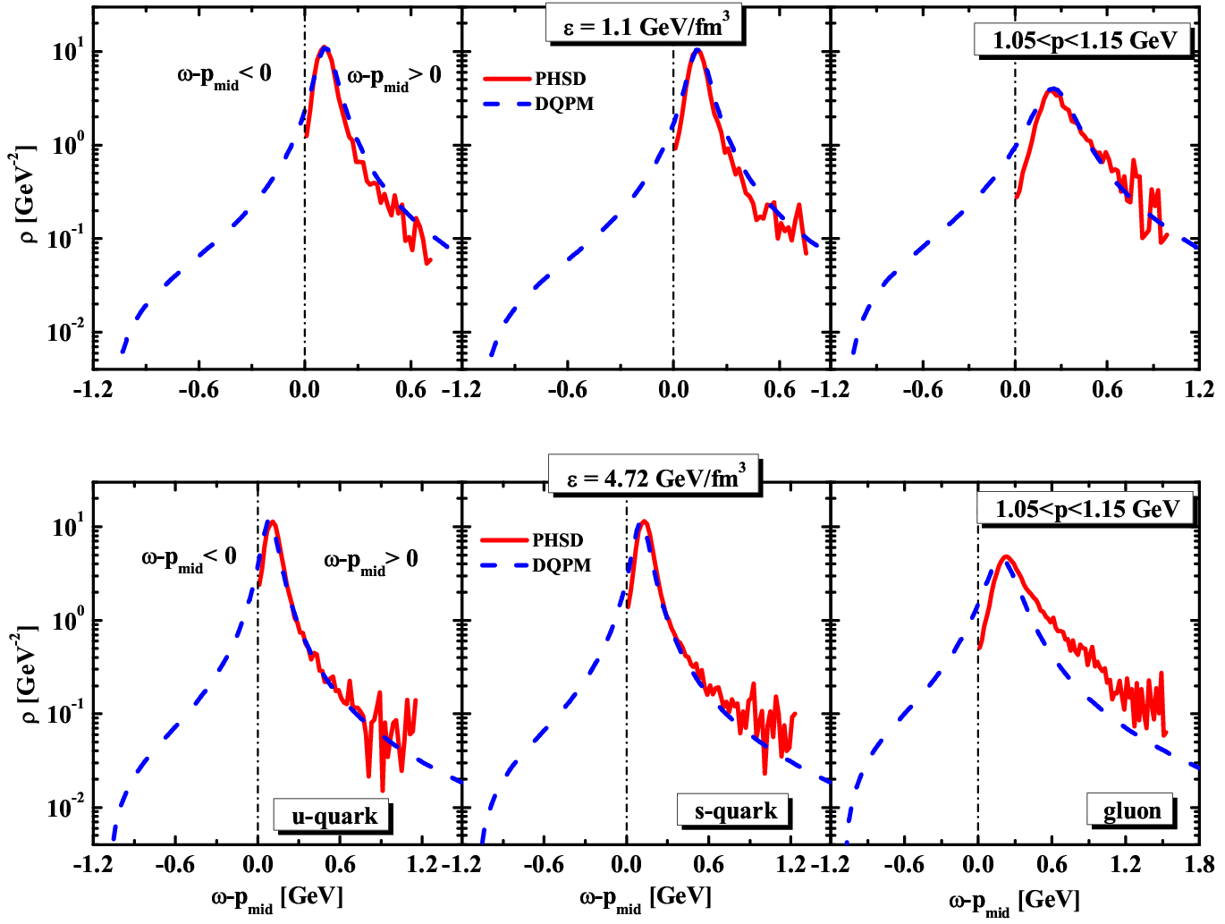
In Fig. 9 we show the dynamical spectral functions for and quarks and gluons as obtained by the PHSD simulations (red solid lines) for “infinite” partonic systems—at energy densities of 1.1 and 4.72 GeV/fm3—and the DQPM assumptions (dashed blue lines) for the spectral functions (30) at the corresponding energy densities of the system.

We find that the dynamical spectral functions of quarks and gluons are generally fairly well described by the DQPM form (30). However, there is a slight deviation visible at high energy density, especially for gluons. This deviation explains the difference between the dynamical results and the DQPM in Fig. 8. The origin of the deviation can be traced back to the inelastic collisions of pairs forming gluons (48) in dense systems. The reactions favor the high-mass part of the gluon spectral function and predominantly populate dynamically the right-hand side from the gluon pole mass since the sum of the pole masses of quarks and antiquarks is larger than the pole mass of the gluon [cf. (29)]. Indeed, let us recall that the inelastic collisions are more important at higher energy densities (cf. Fig. 4). Moreover, from Fig. 10 we see that the elastic scattering rate of gluons is lower than that of quarks. Therefore, the inelastic interaction contributes considerably to the shape of the spectral function of gluons at high energy density, while it is not so important for the quarks at = 1.1 GeV/fm3. In the DQPM it is assumed that the width in the spectral function is independent of the mass, which indeed is found to be a good approximation if elastic scatterings dominate (as in case of the quarks and antiquarks). However, the inelastic interaction of partons in PHSD is dominated by the resonant gluon formation, which dynamically generates a mass-dependent width for the gluon spectral function. This dynamical effect in the gluon width is not incorporated in the DQPM assumption (30). Accordingly, the PHSD simulations for systems in equilibrium supersede the DQPM assumptions but well reproduce the DQPM assumptions in the fermionic sector.


Note that the calculations of in PHSD in the box in the final, equilibrated state allows us to extract the temperature of the “infinite” parton matter. We obtain the final temperature by fitting the parton spectrum obtained by the PHSD simulations with the product of the Bose (Fermi) distribution and a (Lorentzian) spectral function [cf. formula (64)]. In Fig. 11, we show the spectrum of quarks from the PHSD simulations (solid red line) for a system at energy density 4.72 GeV/fm3 in comparison to the fit with different temperatures: = 243 MeV (dashed blue line), = 223 MeV (dash-dotted green line), and = 263 MeV (short-dashed burgundy line). All three curves were normalized to coincide at the peak of the spectral function. One can see that the high-momentum behavior of the distribution is governed by the temperature and that the temperature MeV gives the best fit at the energy density of 4.72 GeV/fm3. We note that the same procedure is repeated for each particle species and each value of the energy density.


The question of whether the equation of state from the PHSD in equilibrium compares reasonably with the lattice data from Ref. [39] can now be aswered. To this end we present in Fig. 12 the equation of state extracted from the PHSD calculations in the box (red stars) in comparison to the respective results from the Wuppertal-Budapest group [39] (blue open circles) as functions of the temperature . We also show the potential energy contribution to the equation of state extracted from the PHSD calculations in the box (green open squares) that is equivalent to the DQPM potential energy density. We find that the equation of state implemented in PHSD is well in agreement with the DQPM and the lQCD results. This finding implies that PHSD dynamically describes systems of quarks, antiquarks, and gluons in equilibrium that have the same properties as explicit QCD calculations on the lattice.
V Finite quark chemical potentials
We have seen in the previous section that the dynamical calculations within PHSD reproduce equilibrium properties of QCD matter as seen in lattice QCD calculations at = 0. Let us now proceed further and study within the dynamical approach the quark and gluon properties at finite quark chemical potential , which are currently not yet well established in lattice QCD calculations.
In Fig. 13 we present the particle abundances of , , and quarks (solid red, short-dashed black, and dash-dotted blue lines, respectively), , , and antiquarks (dotted red, short-dotted black, and short-dash-dotted blue lines, respectively) and gluons (dashed green lines) as functions of time for systems at 1.48 GeV/fm3 and at quark chemical potentials of 50 and 150 MeV. Again chemical equilibrium is achieved for large times but now the abundances of quarks and antiquarks differ considerable (especially for = 150 MeV). A closer inspection also shows that the strangeness equilibration proceeds slower since the amount of flavor-neutral pairs decreases with increasing . Note that the gluon abundance in the equilibrium stage does not depend on the initialization.
The phase boundary in the DQPM (and PHSD) is defined by demanding that the phase transition happens at the same critical energy density for all . The prediction of Fig. 13 might in future be compared to lQCD calculations at finite once physical quark masses can be incorporated into the lQCD calculations.
In Fig. 14 we show for quarks obtained by the PHSD simulations (red solid lines) of “infinite” partonic systems at 1.48 GeV/fm3 and at quark chemical potentials of 50 and 150 MeV. For comparison, we present on the same plots the DQPM assumptions (dashed blue lines) for the respective distributions. The agreement is fairly good since the inelastic channels are further suppressed with increasing . Note that in the present version the DQPM and PHSD treat the quark-hadron transition as a smooth crossover at all . There are, however, some physical arguments in favor of a first-order phase transition at large and for the existence of a critical endpoint for the first-order transition line in the - plane. Presently, we are not able to calculate the properties of a quark-gluon system close to a critical endpoint. It is also not yet clear whether such an endpoint exists.


VI Scaled variance, skewness and kurtosis
In this section we address higher moments of parton distributions in the sQGP within the PHSD approach and study the equilibration of fluctuation observables as well as the size of fluctuations in equilibrium. We recall that various fluctuation observables have been addressed theoretically within lQCD [42, 43, 44, 45] as well as within effective models [46, 47, 48, 49, 50, 51]. Furthermore, some of these observables have been studied experimentally by the various collaborations at the SPS and at RHIC. Most of these have been evaluated in the HSD approach including the individual detector acceptance and experimental biases. For a recent review we refer the reader to Ref. [52] (and references cited therein). The evaluation of the various fluctuations in PHSD is straightforward and in this section performed for .
VI.1 Scaled variances
We start with scaled variance
| (66) |
where is the mean value of the observable averaged over events,
| (67) |
and is the sample variance given by
| (68) |
The standard error of the scaled variance is given by
| (69) | |||||
where
| (70) |
| (71) |
and is the fourth central moment,
| (72) |


In Fig. 15 we show the scaled variances for particle number fluctuations as functions of time for the quarks+antiquarks of all flavors (green open circles), for separate quark flavors— (red squares), (blue down-triangles), and (green up-triangles)—and for gluons (red opened squares), for a system at an energy density of 1.48 GeV/fm3. The same results are presented in Fig. 16 for a system at 4.72 GeV/fm3. Note that in the grand canonical ensemble, i.e., for an equilibrium system with constant temperature (due to the presence of a thermostat) and with thermal fluctuations of the total system energy, one would expect for all particle number fluctuations. On the other hand, for an isolated statistical system the global energy conservation for the microcanonical ensemble leads to a suppression of the particle number fluctuations and thus to (see Ref. [53] for more details). As seen from Figs. 15 and 16 the equilibrium values of are smaller than 1. This can be interpreted as a consequence of the total energy conservation, which is fixed rather more strictly (but still numerically not exactly) in our PHSD box calculations than that in the grand canonical ensemble. In a mixture of different particle species the influence of the global energy conservation on particle number fluctuations is different for different species in the mixture. The suppression effects are stronger for those species that contain larger fractions of the total system energy. The scaled variance of all charged particles (i.e., quarks plus antiquarks of all flavors) is lower than that of gluons or of a single quark flavor. This reflects the larger energy fraction stored in all quarks. For illustration, we show in Fig. 17 the total energy of partons (dash-dotted green lines), the energy of all charged partons (solid red lines), and the energy of gluons (dashed blue lines) as functions of time for systems at energy densities of 1.48 and 4.72 GeV/fm3. We observe that the scaled variances reach a plateau in time for all observables and energy densities. The scaled fluctuations in the gluon number are more pronounced at GeV/fm3 since the fraction of the gluon energy is quite small at this energy density. The difference with respect to the scaled variance of all charged partons decreases with energy due to the higher relative fraction of the gluon energy, as discussed before. Due to the initially lower abundance (thus smaller energy fraction) of strange quarks the respective scaled variance is initially larger but reaches the same asymptotic value as the light quarks in the course of the time evolution. Accordingly, the fluctuations in the fermion number are flavor blind in equilibrium.


It is interesting to study the scaled variance for a cell inside the box as a function of the cell volume. This can easily be achieved by subdividing the total volume fm3 in different subvolumes of equal size and evaluating the scaled variance in each subvolume. Finally an average over the subvolumes is performed. In Fig. 18 we present the scaled variance as functions of in the box for all charged particles (red open circles) and gluons (blue open squares) and for different quarks flavors [ (red open squares), (blue open circles), and (green open triangles) quarks antiquarks] for systems at energy densities of 1.48 and 4.72 GeV/fm3, respectively. The inserts show the observables for larger box sizes by up to about a factor of 8 ( 0.15) in order to explore the thermodynamic limit. Indeed, our calculations demonstrate that the scaled variances no longer change (within statistics) when increasing the volume of the box by up to about an order of magnitude, thus approaching the thermodynamic limit. We recall that for a Poissonian distribution (dash-dotted black lines). The impact of total energy conservation in the box volume is relaxed in the subvolume . This influence becomes weaker for , i.e., . Therefore, in the subvolume the energy fluctuates and these fluctuations behave as in the grand canonical ensemble for . The remaining part of the box plays—in this limit—the role of a thermostat for the cell . This explains the behavior for all scaled variances at large as seen in Fig. 18. Such a behavior can be also expected from the “law of rare events”: the scaled variances for all observables approach the Poissonian limit when one considers only a tiny fraction of all particles in the system.
This observation raises a new question concerning the event-by-event fluctuations in nucleus-nucleus collisions within a viscous hydrodynamical approach. The basic requirement of this approach is that the local cell size—in which a possibly chemical and kinetic equilibrium is achieved—is small compared to the macroscopic dimension of the system; in particular, the gradients in the energy density should be small. In each cell then equilibrium values for averages as well as fluctuations of observables should be considered within the grand canonical treatment. Thus, the influence of the conservation laws (both energy-momentum and charge conservation) gets lost. However, the influence of the global conservation laws on fluctuation observables is by no means negligible even in the thermodynamical limit, if the detector would accept an essential fraction of all particles.


VI.2 Skewness
The skewness [54] characterizes the asymmetry of the distribution function with respect to its average value. If the bulk of the data are at the left and the right tail is stretched out, then the distribution is skewed right or positively skewed; if the peak is toward the right and the left tail is more pronounced, then the distribution is skewed left or negatively skewed. The definition of skewness is as follows:
| (73) |
where and are the second (variance) and third central moments, respectively, with
| (74) |
The skewness of a sample is given by
| (75) |
and its standard error is
| (76) |
In Fig. 19 we show the skewness as functions of time for all charged particles (green open circles) and gluons (red open squares) and for different quarks flavors [ (red squares), (blue down triangles), and (green up triangles) quarks] for a system at 1.48 GeV/fm3. Note that the skewness is equal to zero for symmetric distributions (dash-dotted black lines). We find that in our case the skewness of the number of all charged particles tends to be antisymmetric to the skewness of the number of gluons, but both are compatible with zero for the present accuracy of the calculations. We only show the results for a single energy density since our findings are independent of the energy density.
VI.3 Kurtosis
The height and sharpness of the distribution peak relative to a number is called kurtosis [54]. Higher values of kurtosis indicate a higher, sharper peak; lower values of kurtosis indicate a lower, less distinct peak. The kurtosis is defined as
| (77) |
where is determined by (72). It is equal to 3 for a normal distribution, so often the excess kurtosis is presented which characterizes the deviation from a normal distribution,
| (78) |
The sample excess kurtosis then is defined by
| (79) |
The standard error of the kurtosis is given by
| (80) |
where is determined by (76).
In Fig. 20 we present the excess kurtosis as functions of time for all charged particles (green open circles) and gluons (red open squares) and for different quarks flavors [ (red squares), (blue down triangles), and (green up triangles) quarks] for a system at an energy density of 1.48 GeV/fm3. Note that the excess kurtosis is equal to zero for normal distributions (dash-dotted black lines). The lQCD results from Ref. [44] are nonzero and shown by the dashed orange lines. We find that in our case the excess kurtosis of the number of all charged particles is equal to the excess kurtosis of the number of gluons. However, within statistical errors, the excess kurtosis is compatible with zero as well as with the lQCD results from Ref. [44] for gluons and charged particles. This finding holds for all energy densities considered.
VII Equilibration times
An inspection of the time evolution of the scaled variances in Figs. 15 and 16 shows that the equilibration of the various scaled variances occurs on time scales that are shorter than the time scales for the equilibration of the average values of the observables. In order to quantify this observation we fit the explicit time dependence of the abundances and scaled variances by the function
| (81) |
which defines a characteristic equilibration time . The results of our fits for different observables and energy densities are summarized in Table 1. For all particle species and energy densities, the equilibration time is found to be shorter for the scaled variances than for the average values. This is most pronounced when considering all charged partons but less distinct for strange quarks. Accordingly, scaled variances may achieve an equilibrium, even if the average values of an observable are still out of equilibrium. This finding is reminiscent of strongly interacting quantum systems evaluated on the basis of Kadanoff-Baym equations in Ref. [24], where quantum fluctuations stabilize early in time, i.e., long before a kinetic or chemical equilibrium is achieved.
| Particle type | Equilibration times fm/ | |||
|---|---|---|---|---|
| = 1.48 GeV/fm3 | = 4.72 GeV/fm3 | |||
| abundance | abundance | |||
| 43 | 16 | 21 | 6 | |
| 45 | 14 | 21 | 5 | |
| 35 | 28 | 19 | 17 | |
| gluons | 18 | 5 | 18 | 4 |
| all charged | 18 | 3 | 18 | 2 |
VIII Summary and Conclusions
In this work we have employed the PHSD off-shell transport approach to study partonic systems slightly out of equilibrium as well as in equilibrium in a finite box with periodic boundary conditions, thus simulating “infinite” partonic matter. After a brief recapitulation of off-shell dynamics in phase space we have specified in more detail the ingredients of PHSD, i.e., the retarded self-energies of the partons and the elastic and inelastic cross sections for partons. Furthermore, we have recapitulated the basic equation for the transition from partons to hadrons, i.e., the dynamical hadronization that incorporates all conservation laws as well as an increase in total entropy for a rapidly expanding systems.
We have demonstrated explicitly that partonic systems at energy densities , above the critical energy density Gev/fm3, achieve kinetic and chemical equilibrium in time. Furthermore, the energy density of the partonic system at fixed temperature and quark chemical potential for = 0 is well in line with the lattice QCD calculations [39] in equilibrium. This allows us to study explicit equilibration times for different observables when initializing the partonic system slightly out of equilibrium and also at finite but moderate quark chemical potential 0. Most strikingly, we find that the strangeness degree of freedom equilibrates on time scales that are large compared to the reaction times in relativistic nucleus-nucleus collisions. Nevertheless, the application of PHSD to these reactions from low SPS to top RHIC energies provides a good description of strangeness observables in rapidity and transverse momentum [21, 40]. At first sight this might look like a contradiction; however, the initial nucleon-nucleon collisions in relativistic reactions occur at much larger invariant energies then those in local thermal equilibrium. This makes the strangeness production more effective in collisions. Moreover, the kaon to pion ratio is enhanced at midrapidity—where statistical model fits are performed—due to a narrower rapidity distribution of kaons relative to pions. This effect is seen experimentally and is also present in the nonequilibrium transport (HSD and PHSD) calculations.
In addition to equilibration phenomena of average values for observables such as particle number or charged particle number we have studied the dynamics of fluctuation observables in and out of equilibrium. For all observables the equilibration time is found to be shorter for the scaled variances than for the average values. This is most pronounced when considering all charged partons but less distinct for strange quarks. Accordingly, scaled variances may achieve an equilibrium even if the average values of an observable are still out of equilibrium. This finding is reminiscent of strongly interacting quantum systems evaluated on the basis of Kadanoff-Baym equations [24], where quantum fluctuations stabilize early in time, i.e., long before a kinetic or chemical equilibrium is achieved.
The scaled variances for the fluctuations in the numbers of different partons in the box show an influence of total energy conservation. We observe a suppression of the parton number fluctuations in comparison to the fluctuations in the grand canonical ensemble. Furthermore, by dividing the box into several cells we have calculated the scaled variances of different observables in the cell as functions of the cell size. The scaled variances for all observables approach the Poissonian limit with when the cell volume is much smaller than that of the box. This observation indicates that global conservation laws (for energy-momentum and charges) are not important when one detects only a small fraction from all particles in the system. However, if the fraction of the accepted particles is comparable to that in the whole system, the influence of global conservation laws on fluctuation observables is not negligible even in the thermodynamic limit. We have shown, furthermore, that the scaled variances no longer depend on the size of the box when increasing it up to about an order of magnitude up to 5000 fm3. Accordingly, the continuum limit has approximately been reached in the calculations.
Our analysis of the skewness and kurtosis gives practically vanishing values for these observables in time and especially in equilibrium within the limited statistics achieved. We mention that our results within statistics are also compatible with the lQCD results from Ref. [44]. This issue will have to be readdressed in future along with an evaluation of transport coefficients such as the shear viscosity and bulk viscosity as functions of temperature and quark chemical potential [55].
Acknowledgements
The authors appreciate fruitful discussions with W. Greiner and V. Konchakovski. VO acknowledges financial support through the HIC for FAIR framework of the LOEWE program and Helmholtz Research School for Quark Matter Studies in Heavy Ion Collisions. OL acknowledges financial support through the Margaret Bieber program of the Justus Liebig University of Giessen. The work of MIG was supported by the Humboldt Foundation and the Program of Fundamental Research of the Department of Physics and Astronomy of NAS, Ukraine.
References
- [1] P. Braun-Munziger, J. Stachel, J. P. Wessels, and N. Xu, Phys. Lett. B 344, 43 (1995) ; Phys. Lett. B 365, 1 (1996).
- [2] J. Stachel, Nucl. Phys. A 654, 119c (1999).
- [3] J. Cleymans and H. Satz, Z. Phyc. C 57, 135 (1993).
- [4] J. Sollfank, M. Gazdzicki, U. Heinz, and J. Rafelski, Z. Phys. C 61, 659 (1994).
- [5] F. Becattini, M. Gazdzicki, and J. Sollfank, Eur. Phys. J. C 5, 143 (1998).
- [6] C. Spieles, H. Stöcker, and C. Greiner, Eur. Phys. J. C 2, 351 (1998).
- [7] J. Cleymans, H. Oeschler, and K. Redlich, J. Phys. G 25, 281 (1999).
- [8] W. Broniowski and W. Florkowski, Phys. Rev. C 65, 064905 (2002).
- [9] H. Stöcker and W. Greiner, Phys. Rep. 137, 277 (1986).
- [10] U. Ornik, M. Plumer, B. R. Schlei,D. Strottman, and R .M .Weiner, Phys. Rev. C 54, 1381 (1996).
- [11] S. Bernard et al., Nucl. Phys. A 605, 566 (1996).
- [12] J. Sollfrank, P. Huovinen, M. Kataja, P. V. Ruuskanen, M. Prakash, and R. Venugopalan, Phys. Rev. C 55, 392 (1997).
- [13] P. Koch, B. Müller, and J. Rafelski, Phys. Rep. 142, 167 (1986).
- [14] W. Cassing, V. Metag, U. Mosel, and K. Niita, Phys. Rept. 188, 363 (1990).
- [15] A. Lang, B. Blättel, W. Cassing, V. Koch, U. Mosel, and K. Weber, Z. Phys. A 340, 287 (1991).
- [16] B. Blättel, V. Koch, and U. Mosel, Rep. Progr. Phys. 56, 1 (1993).
- [17] M. Belkacem et al., Phys. Rev. C 58, 1727 (1998).
- [18] L. V. Bravina et al., Phys. Lett. B 434, 379 (1998); J. Phys. G 25, 351 (1999); Phys. Rev. C 60, 024904 (1999); Phys. Rev. C 62, 064906 (2000).
- [19] J. Sollfrank, U. Heinz, H. Sorge, and N. Xu, Phys. Rev. C 59, 1637 (1999).
- [20] E. L. Bratkovskaya et al., Nucl. Phys. A 675, 661 (2000).
- [21] W. Cassing and E. L. Bratkovskaya, Nucl. Phys. A 831, 215 (2009).
- [22] W. Cassing and E. L. Bratkovskaya, Phys. Rev. C 78, 034919 (2008).
- [23] L. P. Kadanoff and G. Baym, Quantum Statistical Mechanics, (Benjamin, New York, 1962).
- [24] S. Juchem, W. Cassing, and C. Greiner, Phys. Rev. D 69, 025006 (2004); Nucl. Phys. A 743, 92 (2004).
- [25] W. Cassing and E. L. Bratkovskaya, Phys. Rept. 308, 65 (1999).
- [26] E. L. Bratkovskaya and W. Cassing, Nucl. Phys. A 619, 413 (1997).
- [27] W. Cassing and S. Juchem, Nucl. Phys. A 665, 377 (2000) ; A 672, 417 (2000).
- [28] E. L. Bratkovskaya and W. Cassing, Nucl. Phys. A 807, 214 (2008).
- [29] W. Cassing, Eur. Phys. J. ST 168, 3 (2009).
- [30] M. Bonitz, Quantum Kinetic Theory, B.G. Teubner, Stuttgart-Leipzig (1998).
- [31] W. Cassing, Nucl. Phys. A 795, 70 (2007).
- [32] W. Cassing, Nucl. Phys. A 791, 365 (2007).
- [33] A. Peshier, B. Kämpfer, O. P. Pavlenko, and G. Soff, Phys. Rev. D 54, 2399 (1996) ; P. Levai and U. Heinz, Phys. Rev. C 57, 1879 (1998) ; A. Peshier, B. Kämpfer, and G. Soff, Phys. Rev. C 61, 045203 (2000), Phys. Rev. D 66, 094003 (2002); M. Bluhm, B. Kämpfer, R. Schulze, D. Seipt, and U. Heinz, Phys. Rev. C 76, 034901 (2007).
- [34] A. Peshier and W. Cassing, Phys. Rev. Lett. 94, 172301 (2005).
- [35] S. Mattiello and W. Cassing, Eur. Phys. J. C 70, 243 (2010).
- [36] A. Peshier, J. Phys. G 31, S371 (2005).
- [37] V. P. Konchakovski, E. L. Bratkovskaya, W. Cassing, V. D. Toneev, and V. Voronyuk, Phys. Rev. C 85, 011902 (2012).
- [38] O. Linnyk, W. Cassing, J. Manninen, E. L. Bratkovskaya, and C. M. Ko, Phys. Rev. C 85, 024910 (2012); O. Linnyk, E. L. Bratkovskaya, V. Ozvenchuk, W. Cassing, and C. M. Ko, Phys. Rev. C 84, 054917 (2011).
- [39] S. Borsanyi et al., JHEP 09, (2010) 073; JHEP 11,(2010) 077.
- [40] E. L. Bratkovskaya, W. Cassing, V. P. Konchakovski, and O. Linnyk, Nucl. Phys. A 856, 162 (2011).
- [41] W. Cassing, Nucl. Phys. A 700, 618 (2002).
- [42] R. V. Gavai and S. Gupta, Phys. Lett. B 696, 459 (2011).
- [43] S. Borsanyi et al., Nucl. Phys. A 855, 253 (2011).
- [44] S. Ejiri, F. Karsch and K. Redlich, Phys. Lett. B 633, 275 (2006).
- [45] M. Cheng et al., Phys. Rev. D 79, 074505 (2009).
- [46] S. Plumari, W. M. Alberico, V. Greco and C. Ratti, Phys. Rev. D 84, 094004 (2011).
- [47] V. Skokov, B. Friman and K. Redlich, Phys. Lett. B 708, 179 (2012)
- [48] B. Friman, F. Karsch, K. Redlich and V. Skokov, Eur. Phys. J. C 71, 1694 (2011).
- [49] N. Strodthoff, B.-J. Schaefer and L. von Smekal, Phys. Rev. D 85, 074007 (2012).
- [50] B.-J. Schaefer and M. Wagner, Phys. Rev. D 85, 034027 (2012)
- [51] M. Nahrgang et al., J. Phys. G 38,124150 (2011).
- [52] V.P. Konchakovski, M. I. Gorenstein, E. L. Bratkovskaya, and W. Greiner, J. Phys. G 37, 073101 (2010).
- [53] V. V. Begun, M. I. Gorenstein, A. P. Kostyuk, and O. S. Zozulya, Phys. Rev. C 71, 054904 (2005); J. Phys. G 32, 935 (2006); V. V. Begun, M. Gazdzicki, M. I. Gorenstein, M. Hauer, V. P. Konchakovski, and B. Lungwitz, Phys. Rev. C 76, 024902 (2007); M. Hauer, V. V. Begun, and M. I. Gorenstein, Eur. Phys. J. C 58, 83 (2008).
- [54] R. A. Fisher and J. J. Wishart, Proc. London Math. Soc., Ser. 2, 33, 195 (1932).
- [55] V. Ozvenchuk, O. Linnyk, M. I. Gorenstein, E. L. Bratkovskaya, and W. Cassing, arXiv: 1212.5393.