Is the Yb2Ti2O7 pyrochlore a quantum spin ice?
Abstract
We use numerical linked cluster (NLC) expansions to compute the specific heat, , and entropy, , of a quantum spin ice model of Yb2Ti2O7 using anisotropic exchange interactions recently determined from inelastic neutron scattering measurements and find good agreement with experimental calorimetric data. In the perturbative weak quantum regime, this model has a ferrimagnetic ordered ground state, with two peaks in : a Schottky anomaly signalling the paramagnetic to spin ice crossover followed at lower temperature by a sharp peak accompanying a first order phase transition to the ferrimagnetic state. We suggest that the two features observed in Yb2Ti2O7 are associated with the same physics. Spin excitations in this regime consist of weakly confined spinon-antispinon pairs. We suggest that conventional ground state with exotic quantum dynamics will prove a prevalent characteristic of many real quantum spin ice materials.
pacs
74.70.-b,75.10.Jm,75.40.Gb,75.30.DsThe experimental search for quantum spin liquids (QSLs), magnetic systems disordered by large quantum fluctuations, has remained unabated for over twenty years [1]. One direction that is rapidly gathering momentum is the search for QSLs among materials that are close relatives to spin ice systems [2], but with additional quantum fluctuations, or quantum spin ice [3, 4].
Spin ices are found among insulating pyrochlore oxides, such as R2M2O7 (R=Ho, Dy; M=Ti, Sn) [5]. In these compounds, the magnetic R rare earth ions sit on a lattice of corner-sharing tetrahedra, experiencing a large single-ion anisotropy forcing the magnetic moment to point strictly “in” or “out” of the two tetrahedra it joins (see. Fig. 1a). Consequently, the direction of a moment can be described by a classical Ising spin [2]. In these materials, the combination of nearest-neighbor exchange and long-range magnetostatic dipolar interactions lead to an exponentially large number of low-energy states characterized by two spins pointing in and two spins pointing out on each tetrahedron (see Fig. 1a). This energetic constraint is equivalent to the Bernal-Fowler ice rule which gives water ice a residual entropy per proton, estimated by Pauling [6] and in good agreement with experiments on water ice [7]. Since they share the same “ice-rule”, the (Ho,Dy)2(Ti,Sn)2O7 pyrochlores also possess a residual low-temperature Pauling entropy [8], hence the name spin ice. The spin ice state is not thermodynamically distinct from the paramagnetic phase. Yet, because of the ice-rules, it is a strongly correlated state of matter – a classical spin liquid of sorts [1, 2].

For infinite Ising anisotropy, quantum effects are absent [2]. However, these can be restored when considering the realistic situation of finite anisotropy. In two closely related papers, Hermele et al. [9] and Castro-Neto et al. [10] considered effective spins one-half on a pyrochlore lattice where the highly degenerate classical spin ice state is promoted via quantum fluctuations to a QSL with fascinating properties. This QSL is described by a compact lattice quantum electrodynamics (QED) -like theory. In this QSL state inherited from the parent classical spin ice, the ice-rules amount to a divergence-free coarse-grained fictitious electric field whose sources are deconfined spinons while the sources of the canonically conjugate field are deconfined monopoles [11], along with a gauge boson (“artificial photon”).
Recent numerical studies have found evidence that QED-like phenomena may be at play in some minimal quantum spin ice (QSI) lattice models [13] – but does the QSI picture apply to real materials? Also, should a QSI state be solely defined by whether or not a QSL state is realized? While a QSI picture has been suggested relevant to the QSL behavior in Tb2Ti2O7 [3] and Pr2M2O7 [4], intense experimental [14, 15, 16, 17, 18, 19, 20, 21] and theoretical [16, 17, 18, 21, 22, 23, 24, 25, 26] interest has recently turned to Yb2Ti2O7 (YbTO), which has been argued to be on the verge of realizing a QSL originating from QSI physics. In fact, the combination of (i) an unexplained transition at 0.24 K [14, 27], (ii) the controversial evidence for long-range order below [28, 29] and (iii) the high sensitivity of the low-temperature ( mK) behavior to sample preparation conditions [19, 20] are all tantalizing evidence that YbTO has a fragile and perhaps unconventional ground state. Thus, explaining YbTO is a key milestone in the study of QSI in a materials context.
In this paper, we first use the numerical linked cluster (NLC) method [30, 31] to calculate the heat capacity, , and entropy, , of a microscopic model for YbTO with exchange parameters, , taken from Ref. [18]. This calculation, which converges down to about 1 K, agrees well with experiments. It demonstrates that YbTO is indeed a spin-half, anisotropic exchange model, with determined from magnon energies in the strong-field polarized paramagnet regime [18]. Our work suggests that a two-peaked structure is natural in YbTO and should be present in the best (“quality”) samples [19, 20]. Below the higher temperature hump near 2 K, the system has a residual comparable to , but without a clean plateau developing upon cooling. We propose that the lower temperature sharp peak in is associated with a strongly first order transition to a ferrimagnetic state. Such a behavior is indeed found in our study when the quantum (non-Ising) exchanges are small. Finally, we argue that despite a conventional ground state, the spin excitations consist of spinon/antispinon pairs connected with (Dirac-like [12]) strings of reversed spins, whose confinement length diverges in the limit of small quantum exchanges. We propose that these excitations should ultimately form the basis for describing what we expect to be highly unconventional inelastic neutron spectra [26].
Model & Method – The anisotropic exchange QSI model is defined by the nearest-neighbor Hamiltonian [18, 25] on the pyrochlore lattice
| (1) | |||||
is a complex unimodular matrix, and [18]. The quantization axis is along the local direction, and refers to the two orthogonal local directions. We take , except when stated otherwise.
Recently Ross et al. [18] used inelastic neutron scattering data in high fields to deduce the exchange parameters for YbTO: , , , and , all in meV. These parameters have also been determined through an analysis of the zero-field energy-integrated paramagnetic neutron scattering [17, 21], but the values of the parameters disagree significantly – an issue that we address in the supplementary material [32].
NLC expansions provide a controlled way of calculating macroscopic properties of a thermodynamic system [30, 31]. By summing up contributions from clusters upto some size, one can obtain properties in the thermodynamic limit, which include all terms in high temperature expansions upto some order. Furthermore, since the contributions of the clusters are entirely included for all temperatures, all short distance physics is fully incorporated, and thus can converge down to lower temperatures than a (high-temperature, ) series expansion [30] in . NLC is particularly suited to the study of spin ice systems. It was recently shown that for classical spin ice models, just first order NLC based on a single tetrahedron, gives and for all within a few percent accuracy [33].
Here, we calculate the thermodynamic properties of the exchange QSI model of Eq. (6) using tetrahedra-based NLC upto 4th order [32]. Euler extrapolations [34] are used to eliminate some alternating pieces in the expansion, which further improves the convergence of the calculations to lower . In zero field, there is only one cluster in each of the first three orders, and three clusters in the fourth order [32]. The different -tensor elements on different sites (expressed in a global frame) [24] mean that many more clusters are needed for calculating field-dependent , magnetization and susceptibility, and these will be presented elsewhere.
Figure 2 shows calculated with different NLC orders. By 4th order, there is good convergence to temperatures below the peak at K. Applying Euler transformations [34] improves the convergence down to slightly below 1 K. The experimental data from Refs. [27], shown for comparison, agree well with the NLC results. Here, we used the mean values of the from Ref. [18] and did not adjust any parameters. Given the variability in the experimental data from one group to another [19, 20, 21, 32], it does not seem useful at this time to search for parameters giving a better fit. This agreement shows that the parameters are not substantially renormalized compared to the high (5 Tesla) field values [18]. Using the of Refs. [17, 21] gives substantially different results [32].


Figure 3 shows calculated by NLC, together with the entropy obtained by integrating data of Ref. [27]. We found the data from Ref. [27] ideally suited to perform this comparison [32]. The entropy converges to lower temperature slightly better than where, with Euler transformations, converges down to about 0.7 K, matching well with the experimental entropy values over the overlapping temperature range.
Perturbative considerations – In order to better understand the properties of this system, we turn to the perturbative regime in Eq. 1 [18, 25]. To second order in , only , by far the largest quantum term for YbTO, leads to a degeneracy-lifting classical potential for different spin-ice configurations. It amounts to a fluctuation-induced ferromagnetic exchange constant [25] between shortest distance spins on the same tetrahedral sublattice that share a neighbor [35]. It leads to the selection of a long-range ordered ground state in which all tetrahedra are in the same configuration and the spins develop a small ferromagnetic moment along one of the cubic directions. This ferrimagnet (FM) lacks the Coulombic physics originally present in the -only spin ice model [36].
To calculate and in the perturbative regime at low , we turn to classical loop Monte Carlo simulations [37] of the model [32]. These reveal a very sharp lower temperature peak signalling a first order phase transition to a state (see Fig. S5 [32]).
Excited states in the perturbative regime: spinons and strings – A surprise of the perturbative treatment is that, while the ground state is classical, the spin-flip excitations remain non-trivial and of quantum nature. This is because, once a spin is flipped in a spin-ice state, creating a spinon/antispinon pair [11], the pair can hop through acting through first order degenerate perturbation theory. Thus, the dispersion in the excited state manifold is , much larger than the dispersion within the low-energy manifold of spin ice states, which is only .
A sketch of a spinon/antispinon pair is shown in Fig. 1b and 1c. Note that only spins inside the tetrahedron “already” containing spinons are flippable in first order degenerate perturbation theory. Hence, the connecting string of misaligned spins can only fluctuate by higher order processes involving closed loops with alternating in-out spins [26]. Thus the renormalized string tension per unit length remains finite and of order . One can estimate the typical string length as the length, , at which the cost of the string becomes comparable to the delocalization energy of the spinon/antispinon pair. The string energy per unit length goes as , whereas the delocalization energy (spinon bandwidth) goes as . This leads to scaling as , which diverges as .
A detailed theory of neutron scattering in this ferrimagnetic phase is not attempted here, but we anticipate it to follow the proposal of Ref. [26]. At temperatures above the transition to the long-range ordered state, the system explores the classical two-in/two-out spin ice states and should display singularities (pinch points, PPs) in neutron scattering [36] rounded off by the finite density of thermally excited spinon/antispinon defects [11, 36]. While the system has thermally smeared PPs above the ferrimagnetic transition and no static PPs well below the transition, it may display some remnant of PPs in the spin dynamics at higher energies. These interesting issues deserve further attention.

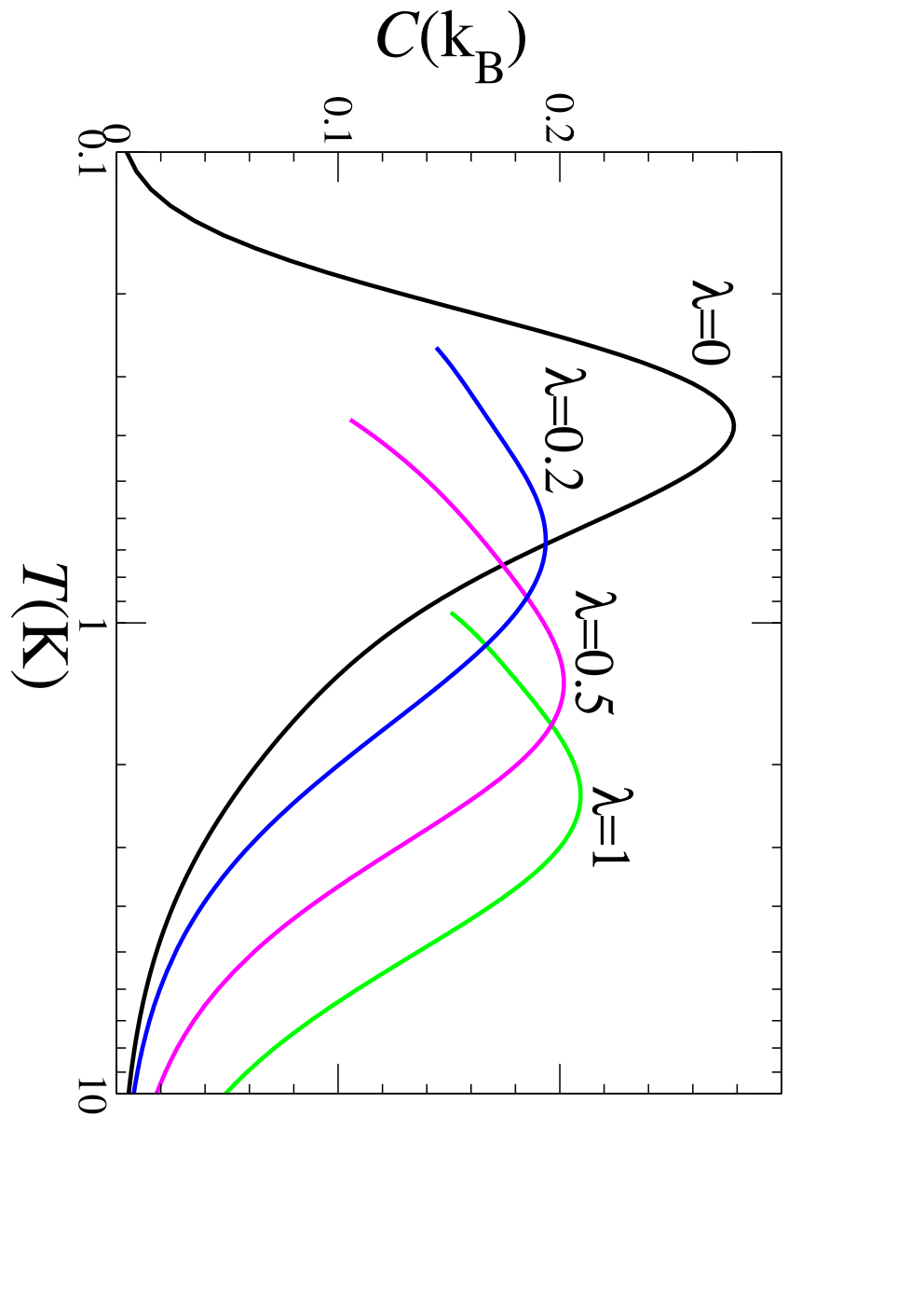
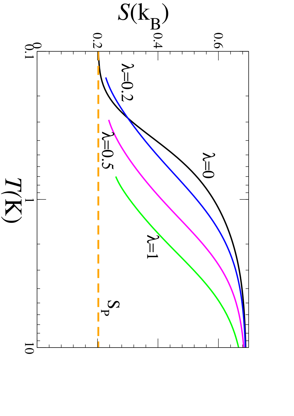
Beyond the regime – Why is the transition temperature of YbTO so low? As discussed by Ross et al. [18], the low peak in is at a temperature lower than mean-field theory by an order of magnitude. Comparing for the quantum model with different with the corresponding classical model with the perturbative value provides a hint of the reason why [32]. It shows that, in the classical model, the long-range order keeps steadily moving up with increased , even beyond the short-range order peak. In contrast, the quantum systems, with different continue to display a short-range order peak and presumably long-range order only occurs at a much lower . Perturbative considerations here have an analogy with strong coupling studies of Mott physics in the Hubbard model, where the Néel temperature first increases with as but then begins decreasing when the system moves away from the perturbative small regime. We propose that a similar non-monotonic arises in this QSI model due to enhanced quantum fluctuations.
Another argument for a reduced comes from considering the temperature dependence of the defect (spinon/antispinon) monopole density, , as calculated by NLC (see Fig. 4 and Figs. S3 and S4 [32]). To illustrate the point, we show the behavior for several different values. Convergence increases to lower , with decreasing , as expected. One finds that as drops below the hump in , displays a plateau-like region, whose value increases steadily with increasing . This indicates that the states within the spin-ice manifold develop large spinon/antispinon spectral weight, thus strongly renormalizing all low energy scales and, presumably, leading to reduced .
Discussion: What constitutes an exchange QSI? – We suggest that a double-peaked with an entropy between the peaks comparable to is the hallmark of an exchange quantum spin ice (QSI). However, one is unlikely to find an exact plateau at outside the perturbative (small ) regime. Such a double-peaked structure and quasi-separation of the energy/temperature scales associated with short and long-range physics has also been suggested for other systems where quantum spin liquid physics may apply [38].
According to the gauge mean-field theory of Ref. [25], at low temperature below which short-range spin ice correlations develop, a system may exhibit either a conventional ferrimagnetic (FM) order, a Coulombic ferromagnet (CFM) or a full-blown quantum spin-liquid (QSL), depending on its quantum exchange parameters. The largest quantum exchange terms in YbTO is , which favors the FM state, which we believe is the origin of the 0.24 K transition in the best samples [28]. It remains to be seen if there are real materials for which , which favors the QSL [9, 10, 25], is the dominant quantum term. Nevertheless, even when the ground state is FM, the excitations remain highly exotic, consisting of spinon-antispinon pairs separated by long strings. This non-trivial feature is derived from the underlying spin-ice physics. Finally, as one notes that is strictly zero for non-Kramers ions (e.g. Pr, Tb) and that virtual crystal field excitations [3] in Tb-based pyrochlores are a fundamentally different pathway from anisotropic superexchange [4] to generate anisotropic couplings between effective spins one-half [3, 4], the prospect to ultimately find a QSI-based QSL among rare-earth pyrochlores [5] is perhaps promising.
Acknowledgements.
This work is supported in part by NSF grant number DMR-1004231, the NSERC of Canada and the Canada Research Chair program (M.G., Tier 1). We acknowledge very useful discussions with B. Javanparast, K. Ross and J. Thompson. We thank P. Dalmas de Réotier for providing specific heat data of Ref. [19].Supplementary Material
This supplement provides the reader with further material to assist with some of the technical materials of the main part paper
Numerical Linked Cluster Method
For the proposed QSI Hamiltonian [18], the numerical linked cluster (NLC) method [30, 31] gives reliable quantitative properties of the system in the thermodynamic limit down to some temperature by developing an expansion in connected tetrahedra that embed in the pyrochlore lattice. For each cluster, we perform an exact diagonalization (ED) and calculate physical quantities from the resulting spectrum and states. Once a property is calculated, the properties of all subclusters are subtracted to get the weight of the cluster denoted as . In the thermodynamic limit, an extensive property, is expressed as
| (2) |
where is the count of the cluster, per lattice site.
We consider all clusters up to four tetrahedra, the largest diagonalization being a 13-site system. All states are required to calculate the partition function and thermodynamic quantities presented below. The particular clusters to fourth order in our expansion are shown in Figure S1.
Computational Requirements
NLC using the tetrahedral basis requires exact diagonalization of increasingly large tetrahedral clusters. Using modern hardware and freely-available linear algebra routines, diagonalizations for clusters of one tetrahedron (four sites) and two tetrahedra (seven sites) could be done in less than a second, while the three-tetrahedron (10-site) cluster still required less than 10 seconds. Computing only the spectrum for a single four-tetrahedron (13-site) cluster required about 1200 seconds and more than 1 GB of memory, while generating the full set of eigenstates required approximately 8 GB of memory. Note that the Hamiltonian of an N-site cluster is a complex Hermitian matrix. Exact diagonalizations of larger systems are, in practice, limited by memory requirements. The next order calculation will have more sites and the memory requirement will grow by a factor of .
Euler Summation
NLC generates a sequence of property estimates with increasing order , where and is some physical quantity calculated at the th order. When such a sequence is found to alternate, its convergence can be improved by Euler Transformation [34]. In general, given alternating terms , the Euler Transform method amounts to estimates,
| (3) |
where is the forward difference operator
| (4) |
Usually, a small number of terms are computed directly, and the Euler transformation is applied to rest of the series. In our case, where direct terms are available to fourth order, we begin the Euler transform after the second order, so that the third and fourth order Euler-transformed property estimates are
| (5) |

Various Hamiltonians and perturbative limit
We use the notation of Ross et al. [18] and define the quantum spin ice Hamiltonian as
| (6) | |||||
The parameters for Yb2Ti2O7 determined by fitting from high-field inelastic neutron (magnon) spectra in Ref. [18] are, measured in meV, , , , and . Two other sets of parameter estimates for Yb2Ti2O7 were determined by fitting the diffused (energy-integrated) neutron scattering using the random phase approximation (RPA) [17, 21]. The values obtained by Thompson et al. [17] are: , , , and , while those obtained by Chang et al. [21] are , , , and . In all cases, the values of the exchange parameters are given in meV. The calculated heat capacity for all these parameters, together with the experimental data on Yb2Ti2O7 from difference groups [20, 19], are shown in Fig. S2. It is clear that the latter two parametrizations by Thompson et al. and Chang et al. do not give a good description of the heat capacity of the material. It is not clear at this time why RPA calculations find such parameters compared to high-field paramagnon spectra [20]. This problem warrants further attention.

In order to explore to what extent quantum mechanical effects are at play in , we introduce a Hamiltonian with rescaled quantum terms as
| (7) |
where is the classical spin-ice Hamiltonian consisting of terms only, while all other terms are included in . The value corresponds to the parameters of Ross et al.[18] In the perturbative regime (), this model maps on to a model with and .
Specific heat and entropy of the system with different values of in 4th order Euler Transform, down to a temperature where rd and th order Euler Transforms agree with each other are shown in Fig. S3 and Fig. S4. Heat capacity of the perturbative classical model, calculated by classical loop Monte Carlo simulations [37] is shown in Fig. S5. Note that while the models with different always have a short-range order peak, in the model, long-range order temperature increases well past the short-range order peak with increasing .
Comparison of the experimental entropy vs NLC results
The entropy difference, between two temperatures and can be obtained by integrating between those two temperatures:
The number of experimental specific heat, , results on Yb2Ti2O7 has rapidly accumulated over the past year or so [21, 19, 20]. Most of these data are somewhat problematic in wanting to assess whether those thermodynamic data hide spin ice phenomenology, associated with a rapid diminution of spinon/antispinon excitation and the concurrent hump at a temperature K as we now discuss.
All of the published data [21, 27, 19, 20] do not go to sufficiently high temperature to extract reliably the limiting high temperature behaviour that would allow one to determine the residual magnetic entropy by integrating upon decreasing starting from the infinite value. One must therefore integrate from low temperature, and assume an entropy value, at some reference (low) temperature, . The apparent large amount of residual entropy below K in the single crystal samples of Refs. [21, 19, 20] make difficult ascribing a reasonable value to . This problem is further compounded by the rising low-temperature nuclear contribution to the total specific heat below about 0.1 K. The very sharp 1st order transition seen in powder powder sample of Ref. [20], without a precise measurement of the associated latent heat also make difficult using those data for comparison of experimental entropy with the calculated by NLC. On the otherhand, the data of Blöte et al. [27] seem the most adequate for comparison with NLC: there is a sharp specific heat peak at K with sufficient temperature resolution that allows integration of over the peak without concern about an associated latent heat. The data are dropping rapidly below , suggesting the opening of an excitation gap, ultimately reaching a low-value that is limited by the “high temperature tail” ( K) of the nuclear contribution. Using the data from Ref. [27], we thus assume that the magnetic part of the specific heat is zero at K, and integrate upward (increasing temperature) up to the highest temperature point available from those data ( K). This results in the data (filled black circles in Fig. 3 in the body of the paper).
It would be highly desirable to repeat this procedure from the data of Refs. [21, 19, 20] which show a sharp peak, but including (magnetic specific heat) data for up to 20 K where the limiting high-temperature regime can be fitted and compared with NLC, along with measurements of the magnetic entropy, .
limit available dataThe data from Working from the reasonable presumption high temperature
Monte Carlo Simulation of the Model
In the perturbative regime of the QSI, we consider the effective Hamiltonian
| (8) |
where are the Ising variables. denotes the sum over the nearest neighbors, denotes the sum over the third nearest neighbors which share a nearest neighbour. Distance-wise there exists another type of third nearest neighbors which do not share a nearest neighbor. For any given spin, there are six third nearest neighbors for both types. Antiferromagnetic drives the spin ice formation in the classical spin ice system, and a small fluctuation-induced ferromagnetic exchange favors the ordering within the spin ice manifold, i.e., all tetrahedra on the same primitive FCC lattice have the same one of the six spin ice states.
Monte Carlo simulations are performed using the Metropolis algorithm. Single spin flip updates are used along with the non-local loop algorithm [37], which restores the ergodicity of the system once it is frozen into the spin ice states. Systems of 128 spins are simulated in a cubic box with periodic boundary conditions. Up to about 78,000 Monte Carlo steps per spin are used in equilibrating the system at a given temperature, with the same number of steps in data sampling. To investigate the calorimetric quantities, fluctuations of the energy are recorded to give the heat capacity:
| (9) |

Calculation of Monopole density
The defect (spinon/antispinon) monopole number , for a cluster, is evaluated as
| (10) | |||||
where is the monopole count in the local basis state . This count is a sum over all the tetrahedra in a cluster, , where
| (11) |
The monopole density is defined as number of monopoles present per site, giving
| (12) |
References
- [1] L. Balents, Nature 464, 199 (2010).
- [2] M. J. P. Gingras, in Introduction to Frustrated Magnetism, (Springer, 2011) arXiv:0903.2772 .
- [3] H. R. Molavian et al., Phys. Rev. Lett. 98, 157204 (2007).
- [4] S. Onoda and Y. Tanaka, Phys. Rev. Lett. 105, 047201 (2010).
- [5] J. S. Gardner et al., Rev. Mod. Phys. 82, 53 (2010).
- [6] L. Pauling, J. Am. Chem. Soc. 57, 2680 (1935).
- [7] W. F. Giauque and J. W. Stout, J. Am. Chem. Soc. 58, 1144 (1936).
- [8] A. P. Ramirez et al., Nature 399, 333 (1999); A. L. Cornelius and J. S. Gardner, Phys. Rev. B 64, 060406 (2001).
- [9] M. Hermele et al., Phys. Rev. B 69, 064404 (2004).
- [10] A. H. Castro Neto et al., Phys. Rev. B 74, 024302 (2006).
- [11] To relate our presentation more directly to the compact lattice QED context set in Refs. [9, 10], in which confinement in three-dimensions is traditionally referred to the strong (electric charge) coupling, we refrain from using the language of “monopoles” employed in Ref. [12] to label local defects in the ice rule of the parent classical spin ice. We use instead the more traditional wording of spinon/antispinon to label finite energy excitations out of the 2in/2out spin ice manifold.
- [12] C. Castelnovo et al., Nature 451, 42 (2008).
- [13] A. Banerjee et al., Phys. Rev. Lett. 100, 047208 (2008); N. Shannon et al., ibid 108, 067204 (2012).
- [14] J. A. Hodges et al., Phys. Rev. Lett. 88, 077204 (2002).
- [15] K. A. Ross et al., Phys. Rev. Lett. 103, 227202 (2009).
- [16] H. B. Cao et al., J. Phys. Condens. Matter 21, 492202 (2009).
- [17] J. D. Thompson et al., Phys. Rev. Lett. 106, 187202 (2011).
- [18] K. A. Ross et al., Phys. Rev. X 1, 021002 (2011).
- [19] A. Yaouanc et al., Phys. Rev. B 84, 172408 (2011).
- [20] K. A. Ross et al., Phys. Rev. B 84, 174442 (2011).
- [21] L.-J. Chang et al., arXiv:1111.5406
- [22] B. Z. Malkin et al., J. Phys. Cond. Matter 22, 276003 (2010).
- [23] S. Onoda, J. Phys.: Conf. Series., 320, 012065 (2011).
- [24] J. D. Thompson et al., J. Phys. Condens. Matter 23, 164219 (2011).
- [25] L. Savary and L. Balents, Phys. Rev. Lett. 108, 037202 (2012)
- [26] Y. Wan and O. Tchernyshyov, arXiv:1201.5314
- [27] H. W. J. Blöte et al., Physica 43, 549 (1969).
- [28] Y. Yasui et al., J. Phys. Soc. Jpn. 72, 3014 (2003).
- [29] J. S. Gardner et al., Phys. Rev. B 70, 180404(R) (2004).
- [30] J. Oitmaa, C. Hamer and W. Zheng, Series Expansion Methods for strongly interacting lattice models (Cambridge University Press, 2006).
- [31] M. Rigol et al., Phys. Rev. Lett. 97, 187202 (2006); Phys. Rev. E 75, 061118 (2007); Phys. Rev. E 75, 061119 (2007).
- [32] See Supplementary Material.
- [33] R. R. P. Singh and J. Oitmaa, arXiv:1112.4439.
- [34] See for example, Numerical Recipes, by W. H. Press et al, Cambridge University Press (1989), Page 133.
- [35] These are geometrically 3rd neighbors on the pyrochlore lattice but not all 3rd neighbors belong to this category.
- [36] C. L. Henley, Annu. Rev. Cond. Matt. Phys. 1, 179 (2010).
- [37] R. G. Melko and M. J. P. Gingras, J. Phys.: Condens. Matter 16, R1277 (2004).
- [38] V. Elser, Phys. Rev. Lett. 62, 2405 (1989). N. Elstner and A. P. Young, Phys. Rev. B 50, 6871 (1994).