Dynamical modeling of high energy heavy ion collisions

Tetsufumi Hirano^1,2 and Yasushi Nara³

Abstract

We present theoretical approaches to high energy nuclear collisions in detail putting a special emphasis on technical aspects of numerical simulations. Models include relativistic hydrodynamics, Monte-Carlo implementation of $k_{T}$ -factorization formula, jet quenching in expanding fluids, a hadronic transport model and the Vlasov equation for colored particles.

1 Introduction

One of the primary purposes of heavy ion physics at ultrarelativistic energies is to explore properties of strongly interacting matter at high temperature and densities, namely, the quark gluon plasma (QGP) [2, 3, 1]. To this purpose, collider experiments of high energy $pp$ , $dA$ and $AA$ collisions have been performed at both Relativistic Heavy Ion Collider (RHIC) in Brookhaven National Laboratory (BNL) and Large Hadron Collider (LHC) in European Organization for Nuclear Research (CERN). It is of particular importance to comprehensively understand space-time evolution of matter created in high energy heavy ion collisions so that one can extract information on the detailed properties of matter from experimental data.

High energy nuclear collisions contain rich physics and exhibit many aspects of dynamics according to relevant energy and time scales. Collisions of two energetic nuclei can be viewed as those of highly coherent dense gluons. Universal behaviors of hadrons and nuclei at the high energy limit are called the color glass condensate (CGC). [4] Just after the collision, longitudinal color electric and magnetic fields between the two passing nuclei, which is called color flux tubes,[5] are produced from CGC initial conditions. Subsequent evolution of these flux tubes is called “glasma” [6]. Long range rapidity correlations in the glasma [7, 8, 9] provide a natural explanation for the ridge structure observed at RHIC [10, 11] and LHC [12]. It was pointed out that instabilities of the gluon fields could play a significant role in the process of thermalization. [13, 14, 15]

A model based on $k_{T}$ -factorization formula [20, 21, 16, 17, 18, 19, 22, 24, 23] or classical Yang-Mills approach [25, 26] reproduces the multiplicity distribution for charged hadrons at RHIC and LHC. However, initial transverse energy per particle is large compared with the experimental data [27, 26, 24]. Glasma evolution based on a 2+1 dimensional classical Yang-Mills simulation does not account for elliptic flow data at RHIC [28]. These facts suggest the necessity of inclusion of further evolution with much stronger interaction, e.g., hydrodynamical evolution. Indeed, a nearly perfect fluid picture [29, 30, 31, 32, 33] turns out to explain large elliptic flow [34] observed at RHIC [35, 36, 37] and LHC,[38, 39, 40] which leads to establishment of a new paradigm “strongly coupled QGP (sQGP)” [2, 3, 41, 42]. These hydrodynamic simulations require very short ( $\mbox{\raisebox{-2.58334pt}{$\stackrel{{\scriptstyle<}}{{\sim}}$}}\>1$ fm/ $c$ ) thermalization time.

Due to expansion and cooling down, a QGP fluid becomes eventually a hadronic gas at a late stage whose evolution can be described by hadronic transport models [43, 31, 44, 45, 46]. Realistic gradual freeze-out both chemically and kinetically can be naturally treated in these models. It is claimed that a QGP fluid picture and a hadron gas picture are demanded to understand $p_{T}$ speactra and differential elliptic flow parameter for identified hadrons simultaneously.[42] For the hadronization processes, it has been claimed that quark recombination/coalescence is important for intermediate transverse momentum region.[47]

On the other hand, high momentum jets are also created in the collision at collider energies. These jets have to traverse the matter in heavy ion collisions and, therefore, interaction with the expanding matter should be treated accordingly. During traveling through the medium, jets interact with soft matter and lose their energies (jet quenching). Therefore, high transverse momentum hadrons are good probes of the bulk matter [48, 49, 50, 51]. Suppression of high transverse momentum hadrons was observed at RHIC [52, 53] and LHC [54]. Disappearance of the away-side peak in azimuthal correlation functions for high transverse momentum hadrons is also observed in central Au+Au collisions at RHIC.[55] High $p_{T}$ suppression in heavy ion collisions turns out to be attributed to the final state interaction because of the Cronin enhancement and the existence of back-to-back correlation in d+Au collisions at midrapidity at RHIC.[56] Theoretical approaches to describe such jet quenching need space-time evolution of parton density through a trajectory of a jet. Hydrodynamical simulation provides such a parton density. A hydro + jet model was proposed in Refs. \citenHirano:2002sc,Hirano:2003hq later followed by Refs. \citenRenk:2006sx,Bass:2008rv,Schenke:2009gb incorporating more realistic models for parton energy loss in a dense medium.

Recent experimental data on higher order anisotropic flow [62, 63, 64] call attention to the importance of initial state fluctuations in heavy ion collisions. It is known that event-by-event fluctuations [65] lead to the higher order anisotropic flow such as triangular flow quantified by third harmonic component of azimuthal angle distributions, and importance of event-by-event simulations with fluctuating initial conditions has been realized [46, 66, 67, 68, 69, 70, 71]. The triangular flow contributes also most of the ridge observed in the two-particle azimuthal correlation. So far only fluctuations from configuration of nucleons inside a colliding nucleus are included in the hydrodynamical simulations. Recently fluctuations from particle production itself are studied [19] by including negative binomial distribution which was obtained by the glasma [72]. It was found that multiplicity fluctuations in $pp$ and $pA$ collisions at midrapidity exhibit Koba-Nielsen-Olsen (KNO) scaling [73]. Fluctuations of particle production increase higher order anisotropy such as triangularity by about 50%[73]. DIPSY event generator which includes the fluctuations arising from dipole evolution also predicts larger higher order anisotropy [74]. Viscous hydrodynamic simulations with fluctuating Glasma initial conditions have been performed recently [75]. Monte-Carlo Glauber type model in which effects of nucleon-nucleon correlations [76, 77] are included was proposed to construct more realistic nuclear configurations for initial conditions of subsequent evolution.

Refer to caption — Figure 1: Dynamical modeling of relativistic heavy ion collisions in view from proper time and energy scale.

As described above, it is needed to incorporate all such different physics consistently to have unified and better understanding of the space-time evolution of the system created in high energy nuclear collisions. Figure 1 shows several important aspects of dynamics of relativistic heavy ion collisions according to time and energy scales. Experimental observables reflect all the history of evolution of matter staring from initial colliding nuclei to final free-streaming hadrons. A first attempt to an integrated approach to the heavy ion collision as a whole was done in Ref. \citenHirano:2004en in which full three dimensional ideal hydrodynamic simulations with initial conditions taken from a CGC based model were performed and parton energy loss was simulated in these expanding fluids. In this review, we present technical and numerical aspects of these important modules for high energy heavy ion collisions; CGC, relativistic hydrodynamics, parton energy loss, hadronic transport models and Vlasov model for colored particles.

This paper is organized as follows. In Sec. 2, we explain in detail numerical aspects of relativistic ideal hydrodynamics in heavy ion collisions. In Sec. 3, Monte-Carlo implementation of the CGC initial conditions based on the $k_{T}$ -factorization formula is discussed. Energy loss of energetic partons in an expanding QGP fluid is briefly discussed in Sec. 4. In Sec. 5, a cascade method and cross sections in the hadronic transport model JAM are briefly summarized. In Sec. 6, we discuss how to solve the Vlasov equation for colored particles by employing the particle-in-cell method. The final section is devoted to summary and conclusion.

2 Relativistic Hydrodynamics

Relativistic hydrodynamics is one of the key dynamical framework to describe the space-time evolution of matter created in relativistic heavy ion collisions. Since the main goal in the physics of relativistic heavy ion collisions is to understand the properties of matter under (local) equilibrium, one can apply hydrodynamics, in which local thermal equilibrium is assumed, to dynamical description of created matter in any cases as a bottom-up approach to see whether the hydrodynamic description works well. In this section, we briefly overview framework of relativistic ideal hydrodynamics and its numerical aspects.

2.1 Relativistic ideal hydrodynamics

Relativistic hydrodynamic equations describe conservation laws of energy and momentum

\displaystyle\partial_{\mu}T^{\mu\nu}(x)

\displaystyle=

\displaystyle 0,

(1)

together with the conservation of charges

\displaystyle\partial_{\mu}N^{\mu}_{i}(x)

\displaystyle=

\displaystyle 0.

(2)

Here $T^{\mu\nu}$ is the energy momentum tensor and $N^{\mu}_{i}$ is the $i$ -th conserved current. With an assumption of ideal hydrodynamics where all dissipative effects are neglected, one can decompose the energy momentum tensor and the conserved currents as

	$\displaystyle T^{\mu\nu}$	$\displaystyle=$	$\displaystyle eu^{\mu}u^{\nu}-P(g^{\mu\nu}-u^{\mu}u^{\nu}),$		(3)
	$\displaystyle N^{\mu}_{i}$	$\displaystyle=$	$\displaystyle n_{i}u^{\mu},$		(4)

where $e$ , $P$ , $n_{i}$ and $u^{\mu}=\gamma(1,\bm{v})=\frac{1}{\sqrt{1-v^{2}}}(1,\bm{v})$ are energy density, pressure, $i$ -th conserved charge density and four flow velocity, respectively. Minkowski metric in this paper is defined as $g^{\mu\nu}=$ diag $(1,-1,-1,-1)$ . Instead of Eqs. (1) and (2), the following expression of the balance equations might be also convenient when compared with non-relativistic equations:

	$\displaystyle\frac{\partial}{\partial t}E+\nabla\cdot(E+P)\bm{v}=0,$		(5)
	$\displaystyle\frac{\partial}{\partial t}M^{k}+\nabla\cdot M^{k}\bm{v}=-\nabla^{k}P,$		(6)
	$\displaystyle\frac{\partial}{\partial t}N_{i}+\nabla\cdot N_{i}\bm{v}=0,$		(7)

where

$\displaystyle E$	$\displaystyle=$	$\displaystyle(e+P)\gamma^{2}-P,$	(8)
$\displaystyle\bm{M}$	$\displaystyle=$	$\displaystyle(e+P)\gamma^{2}\bm{v},$	(9)
$\displaystyle N_{i}$	$\displaystyle=$	$\displaystyle n_{i}\gamma.$	(10)

In ideal hydrodynamic framework, the equation of state plays an important role. First, the hydrodynamic equations (1) and (2) are not closed as a system of partial differential equations: the number of unknowns is 6 (energy density, pressure, charge density and three components of flow velocity) in the case of one conserved charge while the number of equations is 5. So the system is closed when a relation among unknowns, e.g., $P=P(e,n)$ is specified. Second, equations (1) and (2) just describe conservation laws and are the so-called balance equations. Under an assumption of local thermal equilibrium, one can utilize the equation of state $P=P(e,n)$ which only reflects the microscopic dynamics. Since the collective flow is generated by pressure gradient, it is sensitive to the equation of state and the degree of kinetic equilibrium. This is one of the reasons why the collective flow has been focused in relativistic heavy ion collisions.

The equation of state can be taken from results from the first principle calculations of QCD thermodynamics, namely, lattice QCD. [79, 80, 81, 82] A few comments regarding this are in order here.

1.

In the current status of the lattice QCD results, the equation of state is not so reliable in the low temperature region ( $T\mbox{\raisebox{-2.58334pt}{$\stackrel{{\scriptstyle<}}{{\sim}}$}}\>100$ MeV). Then one can connect lattice QCD results at high temperature with results from the hadronic resonance gas model at low temperature. [83, 84] Practically, this is also demanded from a point of view of freezeout at which all hydrodynamic variables are switched to a particle picture employing the Cooper-Frye formula.[85] Energy, momentum and charges are conserved in this formula only when the hadronic resonance gas picture is valid.
2.

Monte-Carlo calculations of lattice QCD at finite baryonic chemical potential [86] suffer from a severe issue due to the so-called sign problem. The equation of state at finite baryon density, however, would be demanded in lower collision energies or in forward/backward rapidity regions.
3.

Even if results will become reliable in the low temperature region and/or finite baryon density region in lattice QCD, there is an issue on chemical freezeout since all thermodynamic variables are obtained for thermally as well as chemically equilibrated states. In the actual hadronic matter created in relativistic heavy ion collisions, chemical composition of hadrons is almost frozen during expansion according to statistical model analyses. Thus, each hadron acquires its chemical potential associated with the approximated conserved number of the hadron below chemical freezeout temperature. Again, the hadronic resonance gas model with finite chemical potential [33, 87, 88, 89, 90] is needed to describe the space-time evolution of hadronic matter in hydrodynamics. Since the matter is already diluted due to expansion, one can instead use the hadronic cascade model for a better dynamical description of hadronic matter. This will be discussed in Sec. 5.

2.2 Numerical aspects of relativistic ideal hydrodynamics

In this subsection, we review a numerical scheme to solve relativistic hydrodynamic equations for perfect fluids. We first discretize relativistic hydrodynamic equations in Cartesian coordinate to solve numerically in Sec. 2.2.1. We also discuss the conventional way to treat multi-dimensional problem, namely, the operator splitting method. After that, we introduce the piecewise parabolic method (PPM), [91] which is known as a robust algorithm against strong shock waves, to relativistic hydrodynamic equations in Sec. 2.2.2. In practice, one needs to convert a set of numerical solutions to physical quantities such as thermodynamic variables and flow velocity. The procedure to obtain them is explained in Sec. 2.2.3. Finally, we discuss hydrodynamic equations in relativistic coordinate (proper time $\tau$ and space-time rapidity $\eta_{s}$ ) in Sec. 2.2.4.

2.2.1 Discretization and the operator splitting method

In the Cartesian coordinate, hydrodynamic equations (1) and (2) for a relativistic perfect fluid with one conserved charge (e.g., baryon charge) can be written as

\displaystyle\partial_{t}\begin{pmatrix}U_{1}\\ U_{2}\\ U_{3}\\ U_{4}\\ U_{5}\\ \end{pmatrix}+\nabla\cdot\begin{pmatrix}U_{1}\\ U_{2}\\ U_{3}\\ U_{4}\\ U_{5}\\ \end{pmatrix}\bm{v}+\begin{pmatrix}\partial_{x}P\\ \partial_{y}P\\ \partial_{z}P\\ \nabla\cdot P\bm{v}\\ 0\\ \end{pmatrix}=0,

(11)

where

\displaystyle\begin{pmatrix}U_{1}\\ U_{2}\\ U_{3}\\ U_{4}\\ U_{5}\\ \end{pmatrix}

\displaystyle=

\displaystyle\begin{pmatrix}\gamma^{2}(e+P)v_{x}\\ \gamma^{2}(e+P)v_{y}\\ \gamma^{2}(e+P)v_{z}\\ \gamma^{2}(e+P)-P\\ \gamma n_{B}\\ \end{pmatrix}.

(12)

These equations can be summarized as a continuity equation in the following form

\displaystyle\partial_{t}U_{J}(t,\bm{x})+\sum_{i=x,y,z}\partial_{i}F_{iJ}\left[U_{J}(t,\bm{x})\right]

\displaystyle=

\displaystyle 0,\quad(J=1,\cdots,5).

(13)

For example, $F_{x1}=U_{1}v_{x}+P$ , $F_{y1}=U_{1}v_{y}$ , $F_{x2}=U_{2}v_{x}$ and so on.

One discretizes Eq. (13) and write in a general form

\displaystyle[U_{J}]_{ijk}^{n+1}=[U_{J}]_{ijk}^{n}-\frac{\Delta t}{\Delta x}\sum_{l=x,y,z}G_{lJ}\left[[U_{J}]_{ijk}^{n}\right],

(14)

or more simply,

\displaystyle U_{ijk}^{n+1}=U_{ijk}^{n}-\frac{\Delta t}{\Delta x}G_{l}\left[U_{ijk}^{n}\right].

(15)

Here $n$ is a time step and $i$ , $j$ and $k$ are fluid cell indices in $x$ , $y$ and $z$ direction, respectively. $\Delta t$ and $\Delta x$ are mesh sizes in temporal and spatial direction, respectively, which should obey $C\leq 1$ in relativistic cases where $C=\Delta t/\Delta x$ is the Courant number (Note that we have employed natural unit $c=1$ ). We here assume isotropic lattice in three dimensions. One can cope with these kinds of multi-dimensional equations by employing the operator splitting method. In this method, the operators are split into three sequential one-dimensional spatial steps:

$\displaystyle\tilde{U}_{ijk}$	$\displaystyle=$	$\displaystyle U_{ijk}^{n}-\frac{\Delta t}{\Delta x}G_{x}[U_{ijk}^{n}],$	(16)
$\displaystyle\hat{U}_{ijk}$	$\displaystyle=$	$\displaystyle\tilde{U}_{ijk}-\frac{\Delta t}{\Delta x}G_{y}[\tilde{U}_{ijk}],$	(17)
$\displaystyle U_{ijk}^{n+1}$	$\displaystyle=$	$\displaystyle\hat{U}_{ijk}-\frac{\Delta t}{\Delta x}G_{z}[\hat{U}_{ijk}].$	(18)

To avoid numerical errors on spatial anisotropy, the above process is cyclically changed every time step. Now the problem in three dimensional space reduces to the one in one dimension. Hereafter in this subsection we concentrate our discussion on solving hydrodynamic equation in one-dimensional space.

2.2.2 Piecewise parabolic method

As a robust numerical algorithm to solve hydrodynamic equations, we review the piecewise parabolic method (PPM)[91] in this paper. PPM was employed for the first time in the physics of relativistic heavy ion collisions in Ref. \citenHirano:2000eu to solve relativistic hydrodynamic equations in Cartesian coodinate and later applied to problems in relativistic $\tau$ - $\eta_{s}$ coordinate in Ref. \citenHirano:2001eu. PPM is categorized in the so-called Godunov’s method. Godunov made use of a Riemann’s shock tube problem, approximated a solution of interpolating two discontinuous states to a constant one and obtained it using conservation equations. PPM is, so to speak, a higher order extension of the Godunov’s approach. As a consequence, PPM allows one to describe a hydrodynamic response to steep profile very efficiently. For details, see Ref. \citenColella:1982ee. For other algorithms such as SHASTA and rHLLE, see also Ref. \citenSchneider:1993gd

For a given set of discrete values of fields $\{U_{j}^{n}\}$ at time step $n$ , an interpolation function, $U_{j}(x)$ , can be defined as

\displaystyle U_{j}^{n}=\frac{1}{\Delta x}\int_{x_{j-1/2}}^{x_{j+1/2}}U_{j}(x)dx,

(19)

where $U_{j}(x)$ is assumed to be continuous and a parabolic function in $x_{j}-\Delta x/2=x_{j-1/2}<x<x_{j+1/2}=x_{j}+\Delta x/2$ . Then one can parametrize $U_{j}(x)$ as

$\displaystyle U_{j}(x)$	$\displaystyle=$	$\displaystyle U_{L,j}+\frac{x-x_{j-1/2}}{\Delta x}\left[\Delta U_{j}+U_{6,j}\left(1-\frac{x-x_{j-1/2}}{\Delta x}\right)\right],$	(20)
$\displaystyle\Delta U_{j}$	$\displaystyle=$	$\displaystyle U_{R,j}-U_{L,j},$	(21)
$\displaystyle U_{6,j}$	$\displaystyle=$	$\displaystyle 6\left[U_{j}^{n}-\frac{1}{2}\left(U_{R,j}+U_{L,j}\right)\right],$	(22)

where $U_{j}(x_{j-1/2})=U_{L,j}$ and $U_{j}(x_{j+1/2})=U_{R,j}$ to be determined as follows.

As default values at cell boundary, one puts

	$\displaystyle U_{R,j}$	$\displaystyle=$	$\displaystyle\frac{7}{12}(U_{j}^{n}+U_{j+1}^{n})-\frac{1}{12}(U_{j+2}^{n}+U_{j-1}^{n}),$		(23)
	$\displaystyle U_{L,j}$	$\displaystyle=$	$\displaystyle\frac{7}{12}(U_{j-1}^{n}+U_{j}^{n})-\frac{1}{12}(U_{j+1}^{n}+U_{j}^{n}),$		(24)

using discretized solutions $\{U_{j}^{n}\}$ at time step $n$ . These values are obtained as follows. Assuming integral of $U(x)$ can be parameterized using a quartic function (here $U(x)$ is rather defined globally at least in $x_{j-3/2}<x<x_{j+5/2}$ ),

	$\displaystyle\mathcal{U}(x)$	$\displaystyle=$	$\displaystyle\int^{x}U(x^{\prime})dx^{\prime}$		(25)
		$\displaystyle=$	$\displaystyle ax^{4}+bx^{3}+cx^{2}+dx+e,$		(26)

we calculate the value at the cell boundary $x=x_{j+1/2}$ as

\displaystyle U(x_{j+1/2})

\displaystyle=

\displaystyle\left.\frac{d\mathcal{U}}{dx}\right|_{x=x_{j+1/2}}

(27)

Only when we solve this problem, one can suppose $x_{j+1/2}=0$ and $\mathcal{U}(x=x_{j-3/2})=0$ without loss of generality. Then, $U(x_{j+1/2})=d$ . We obtain the following coupled equations,

$\displaystyle\mathcal{U}(2\Delta x)$	$\displaystyle=$	$\displaystyle\int_{x_{j-3/2}}^{x_{j+3/2}}U(x)dx=\left(U_{j-1}+U_{j}+U_{j+1}+U_{j+2}\right)\Delta x,$	(28)
$\displaystyle\mathcal{U}(\Delta x)$	$\displaystyle=$	$\displaystyle(U_{j-1}+U_{j}+U_{j+1})\Delta x,$	(29)
$\displaystyle\mathcal{U}(0)$	$\displaystyle=$	$\displaystyle(U_{j-1}+U_{j})\Delta x,$	(30)
$\displaystyle\mathcal{U}(-\Delta x)$	$\displaystyle=$	$\displaystyle U_{j-1}\Delta x,$	(31)
$\displaystyle\mathcal{U}(-2\Delta x)$	$\displaystyle=$	$\displaystyle 0.$	(32)

Solving these equations with respect to $a,\cdots$ and $e$ , we finally obtain Eq. (23).

However, the value has to be reset in some cases. The interpolation function $U_{j}(x)$ is imposed to be monotonic in $x_{j-1/2}<x<x_{j+1/2}$ : $U_{j}(x)$ should take its value between $U_{R,j}$ and $U_{L,j}$ . In fact, $U_{j}(x)$ does not obey this condition either when $U_{j}^{n}$ is a local minimum or maximum or when $U_{j}(x)$ has an extreme even though $U_{j}^{n}$ is between $U_{R,j}$ and $U_{L,j}$ . From Eq. (20), this is the case when $\mid\Delta U_{j}\mid\geq\mid U_{6,j}\mid$ . The following replacement is made in these cases:

$\displaystyle U_{R,j},U_{L,j}$	$\displaystyle\rightarrow$	$\displaystyle U_{j}^{n}\quad\mbox{if}\quad(U_{R,j}-U_{j}^{n})(U_{j}^{n}-U_{L,j})\leq 0,$	(33)
$\displaystyle U_{L,j}$	$\displaystyle\rightarrow$	$\displaystyle 3U_{j}^{n}-2U_{R,j}\quad\mbox{if}\quad\Delta U_{j}U_{6,j}>(\Delta U_{j})^{2},$	(34)
$\displaystyle U_{R,j}$	$\displaystyle\rightarrow$	$\displaystyle 3U_{j}^{n}-2U_{L,j}\quad\mbox{if}\quad\Delta U_{j}U_{6,j}<-(\Delta U_{j})^{2}.$	(35)

In the case of heavy ion collisions, fluids sometime can be surrounded by vacuum in which $U_{j}^{n}$ vanishes. In this case, both $U_{L,j}$ and $U_{R,j}$ are set to be zero. When the default value calculated using Eq. (20) becomes negative, it is also set to be zero.¹¹ 1 This might have been too strict for $U_{5}$ to be set since it could be negative. However, if initial $U_{5}$ is positive, it keeps to be positive in this fluid element. Therefore there is no problem in ordinary cases.

Using $U_{L,j}$ and $U_{R,j}$ determined above, one calculates thermodynamic variables ( $e_{L,R}$ and $P_{L,R}$ ), sound velocity ( $c_{L,R}$ ) and flow velocity ( $v_{L,R}$ ). We will discuss how to obtain these variables from numerical solutions $U$ in the next subsection. Average values of interpolation function around the cell interfaces are

	$\displaystyle\bar{U}_{L,j+1}$	$\displaystyle=$	$\displaystyle\frac{1}{\mid b_{r,j+1/2}\mid\Delta t}\int_{x_{j+1/2}}^{x_{j+1/2}+\mid b_{r,j+1/2}\mid\Delta t}U_{j+1}(x)dx,$		(36)
	$\displaystyle\bar{U}_{R,j}$	$\displaystyle=$	$\displaystyle\frac{1}{\mid b_{l,j+1/2}\mid\Delta t}\int_{x_{j+1/2}-\mid b_{l,j+1/2}\mid\Delta t}^{x_{j+1/2}}U_{j}(x)dx$		(37)

$b_{r}$ and $b_{l}$ are signal velocities

$\displaystyle b_{r,j+1/2}$	$\displaystyle=$	$\displaystyle\mbox{max}\left(0,\frac{v_{L,j+1}+c_{L,j+1}}{1+v_{L,j+1}c_{L,j+1}},\frac{\bar{v}_{j+1/2}+\bar{c}_{j+1/2}}{1+\bar{v}_{j+1/2}\bar{c}_{j+1/2}}\right),$	(38)
$\displaystyle b_{l,j+1/2}$	$\displaystyle=$	$\displaystyle\mbox{min}\left(0,\frac{v_{R,j}-c_{R,j}}{1-v_{R,j}c_{R,j}},\frac{\bar{v}_{j+1/2}+\bar{c}_{j+1/2}}{1+\bar{v}_{j+1/2}\bar{c}_{j+1/2}}\right),$	(39)
$\displaystyle\bar{v}_{j+1/2}$	$\displaystyle=$	$\displaystyle\frac{1}{2}(v_{R,j}+v_{L,j+1}),$	(40)
$\displaystyle\bar{c}_{j+1/2}$	$\displaystyle=$	$\displaystyle\frac{1}{2}(c_{R,j}+c_{L,j+1}).$	(41)

Notice that $b_{l,j+1/2}\leq 0$ . When a fluid cell is located next to vacuum, e.g., $(U_{4})_{j}\neq 0$ and $(U_{4})_{j+1}=0$ , we set $b_{r}=1$ . Please notice that the subscripts $R$ and $L$ represent, respectively, the values of right side and left side at each cell, but that the subscripts $r$ and $l$ denote, respectively, the values of right side and left side at each cell boundary. Inserting Eq. (20) into Eqs. (36) and (37), we obtain

	$\displaystyle\bar{U}_{L,j+1}$	$\displaystyle=$	$\displaystyle U_{L,j+1}+\frac{b_{r,j+1/2}\Delta t}{2\Delta x}\left[\Delta U_{j+1}+\left(1-\frac{2b_{r,j+1/2}\Delta t}{3\Delta x}\right)U_{6,j+1}\right],$		(42)
	$\displaystyle\bar{U}_{R,j}$	$\displaystyle=$	$\displaystyle U_{R,j}-\frac{b_{l,j+1/2}\Delta t}{2\Delta x}\left[\Delta U_{j}-\left(1-\frac{2b_{l,j+1/2}\Delta t}{3\Delta x}\right)U_{6,j}\right].$		(43)

By using these average values above, we solve the Riemann problem at each cell boundary. The solution becomes complicated in general. Thus, in the Godunov-type algorithm, one approximates the solution to a constant value $U_{lr}$ which fulfills the conservation law. One rewrites the hydrodynamic equations in their integral form:

			$\displaystyle\int_{x_{j}}^{x_{j+1/2}}[U(x,t_{n}+\Delta t/2)-U(x,t_{n})]dx$		(44)
		$\displaystyle=$	$\displaystyle-\int_{t_{n}}^{t_{n}+\Delta t/2}\left[F(U(x_{j+1/2},t))-F(U(x_{j},t))\right]dt$		(44)

The integration can be easily done by assuming $U(x_{j})=\bar{U}_{R,j}$ = const. in $t_{n}<t<t_{n}+\Delta t/2$ . The result becomes

\displaystyle(\bar{U}_{R,j}-U_{lr})b_{l,j+1/2}\frac{\Delta t}{2}

\displaystyle=

\displaystyle-\left[F(U_{lr})-F(\bar{U}_{R,j})\right]\frac{\Delta t}{2}.

(45)

One also integrates the hydrodynamic equations over $x_{j+1/2}<x<x_{j+1}$

			$\displaystyle\int_{x_{j+1/2}}^{x_{j+1}}[U(x,t_{n}+\Delta t/2)-U(x,t_{n})]dx$		(46)
		$\displaystyle=$	$\displaystyle-\int_{t_{n}}^{t_{n}+\Delta t/2}\left[F(U(x_{j+1},t))-F(U(x_{j+1/2},t))\right]dt$		(46)

and obtains

\displaystyle(U_{lr}-\bar{U}_{L,j+1})b_{r,j+1/2}\frac{\Delta t}{2}

\displaystyle=

\displaystyle-\left[F(\bar{U}_{L,j+1})-F(U_{lr})\right]\frac{\Delta t}{2}.

(47)

From Eqs. (45) and (47), one obtains $U_{lr}$ and $F(U_{lr})$

$\displaystyle U_{lr}$	$\displaystyle=$	$\displaystyle\frac{F(\bar{U}_{R,j})-F(\bar{U}_{L,j+1})-b_{l,j+1/2}\bar{U}_{R,j}+b_{r,j+1/2}\bar{U}_{L,j+1}}{b_{r,j+1/2}-b_{l,j+1/2}}$	(48)
$\displaystyle F(U_{lr})$	$\displaystyle=$	$\displaystyle F_{j+1/2}$
	$\displaystyle=$	$\displaystyle\frac{b_{r,j+1/2}F(\bar{U}_{R,j})-b_{l,j+1/2}F(\bar{U}_{L,j+1})+b_{r,j+1/2}b_{l,j+1/2}(\bar{U}_{L,j+1}-\bar{U}_{R,j})}{b_{r,j+1/2}-b_{l,j+1/2}}$

Finally, the solution at the next time step leads to

\displaystyle U_{j}^{n+1}

\displaystyle=

\displaystyle U_{j}^{n}-\frac{\Delta t}{\Delta x}(F_{j+1/2}-F_{j-1/2})

(50)

The key difference between the conventional Godunov scheme and the present method is using the average values $\bar{U}_{R,j}$ and $\bar{U}_{L,j+1}$ instead of $U_{j}$ and $U_{j+1}$ to gain accuracy of numerical solutions since numerical fluxes using $U_{j}$ or $U_{j+1}$ are often overestimated, in particular, in the case of steep profiles.

2.2.3 Thermodynamic variables and flow velocity

We transform from thermodynamic variables and flow velocity to variables to solve the relativistic hydrodynamic equations numerically in Eq. (12). Hence we need to transform back to thermodynamic variables from numerical solutions $U_{J}$ . From Eq. (12),

$\displaystyle v=\mid\bm{v}\mid$	$\displaystyle=$	$\displaystyle\frac{\mid\bm{U}\mid}{U_{4}+P(e,n_{B})},$	(51)
$\displaystyle e$	$\displaystyle=$	$\displaystyle U_{4}-\bm{U}\cdot\bm{v},$	(52)
$\displaystyle n_{B}$	$\displaystyle=$	$\displaystyle U_{5}\sqrt{1-v^{2}},$	(53)
$\displaystyle\bm{U}$	$\displaystyle=$	$\displaystyle(U_{1},U_{2},U_{3}).$	(54)

For a given equation of state, $P=P(e,n_{B})$ , and numerical solutions, $U_{J}$ , Eq. (51) with Eqs. (52) and (53) becomes a non-linear equation with respect to $v$ . Therefore, one has to solve it numerically using, e.g., the bi-section method. Once the solution $v$ is obtained from Eq. (51), it is easy to obtain energy density and baryon density from Eqs. (52) and (53) and, consequently, pressure from the equation of state.

2.2.4 Hydrodynamic equations in relativistic coordinate

It is more appropriate to write down relativistic hydrodynamic equations in an expanding coordinate in the case of relativistic heavy ion collisions:

\displaystyle\partial_{\tau}\begin{pmatrix}U_{1}\\ U_{2}\\ U_{3}\\ U_{4}\\ U_{5}\\ \end{pmatrix}+\nabla\cdot\begin{pmatrix}U_{1}\\ U_{2}\\ U_{3}\\ U_{4}\\ U_{5}\\ \end{pmatrix}\tilde{\bm{v}}+\begin{pmatrix}\tau\partial_{x}P\\ \tau\partial_{y}P\\ \partial_{\eta_{s}}P\\ \tau\nabla\cdot P\tilde{\bm{v}}\\ 0\\ \end{pmatrix}+\begin{pmatrix}0\\ 0\\ U_{3}/\tau\\ U_{4}\tilde{v}_{\eta_{s}}^{2}/\tau+P(1+\tilde{v}_{\eta_{s}}^{2})\\ 0\\ \end{pmatrix}=0,

(55)

where

\displaystyle\begin{pmatrix}U_{1}\\ U_{2}\\ U_{3}\\ U_{4}\\ U_{5}\\ \end{pmatrix}

\displaystyle=

\displaystyle\begin{pmatrix}\tau\tilde{\gamma}^{2}(e+P)\tilde{v}_{x}\\ \tau\tilde{\gamma}^{2}(e+P)\tilde{v}_{y}\\ \tau\tilde{\gamma}^{2}(e+P)\tilde{v}_{z}\\ \tau\tilde{\gamma}^{2}(e+P)-\tau P\\ \tau\tilde{\gamma}n_{B}\\ \end{pmatrix}.

(56)

where proper time $\tau=\sqrt{t^{2}-z^{2}}$ , space-time rapidity $\eta_{s}=(1/2)\ln[(t+z)/(t-z)]$ and $\nabla=(\partial_{x},\partial_{y},\partial_{\eta_{s}}/\tau)$ . Flow velocities and fluid rapidity in this coordinate are, respectively,

$\displaystyle\tilde{v}_{x}$	$\displaystyle=$	$\displaystyle\frac{\cosh Y_{f}}{\cosh(Y_{f}-\eta_{s})}v_{x},$	(57)
$\displaystyle\tilde{v}_{y}$	$\displaystyle=$	$\displaystyle\frac{\cosh Y_{f}}{\cosh(Y_{f}-\eta_{s})}v_{y},$	(58)
$\displaystyle\tilde{v}_{\eta_{s}}$	$\displaystyle=$	$\displaystyle\tanh(Y_{f}-\eta_{s}),$	(59)
$\displaystyle\tilde{\gamma}$	$\displaystyle=$	$\displaystyle\frac{1}{\sqrt{1-\tilde{v}_{x}^{2}-\tilde{v}_{y}^{2}-\tilde{v}_{\eta_{s}}^{2}}}.$	(60)

where $Y_{f}=\frac{1}{2}\ln\left[(1+v_{z})/(1-v_{z})\right]$ .

Equation (55) is quite similar to Eq. (11) except for existence of the last term in the left hand side which is a source term due to expanding coordinate. Therefore, one can utilize the same PPM algorithm by adding source terms in the cycle of operator splitting.

One can obtain thermodynamic variables and flow velocities from the following relations:

$\displaystyle\tilde{v}=\mid\tilde{\bm{v}}\mid$	$\displaystyle=$	$\displaystyle\frac{\mid\bm{U}\mid/\tau}{U_{4}/\tau+p(e,n_{B})},$	(61)
$\displaystyle e$	$\displaystyle=$	$\displaystyle\frac{U_{4}}{\tau}-\frac{\mid\bm{U}\mid}{\tau}\cdot\mid\tilde{\bm{v}}\mid,$	(62)
$\displaystyle n_{B}$	$\displaystyle=$	$\displaystyle\frac{U_{5}}{\tau}\sqrt{1-\mid\tilde{\bm{v}}\mid^{2}}.$	(63)

Inserting Eqs. (62) and (63) into Eq. (61), we first solve an implicit equation for $\mid\tilde{\bm{v}}\mid$ numerically and then obtain $e$ , $n_{B}$ and $P=P(e,n_{B})$ . From numerical solutions $U_{J}$ , we also obtain each component of $\tilde{\bm{v}}$ :

\displaystyle\tilde{\bm{v}}=\frac{1}{U_{4}+\tau P}(U_{1},U_{2},U_{3}).

(64)

Velocities in the Cartesian coordinate are obtained from $\tilde{\bm{v}}$

$\displaystyle v_{x}$	$\displaystyle=$	$\displaystyle\frac{\cosh(Y_{f}-\eta_{s})}{\cosh Y_{f}}\tilde{v}_{x},$	(65)
$\displaystyle v_{y}$	$\displaystyle=$	$\displaystyle\frac{\cosh(Y_{f}-\eta_{s})}{\cosh Y_{f}}\tilde{v}_{y},$	(66)
$\displaystyle v_{z}$	$\displaystyle=$	$\displaystyle\frac{\tilde{v}_{\eta_{s}}\cosh\eta_{s}+\sinh\eta_{s}}{\cosh\eta_{s}+\tilde{v}_{\eta_{s}}\sinh\eta_{s}}=\tanh Y_{f},$	(67)
$\displaystyle\gamma$	$\displaystyle=$	$\displaystyle\frac{\cosh Y_{f}}{\cosh(Y_{f}-\eta_{s})}\tilde{\gamma},$	(68)

where $Y_{f}=\tanh^{-1}\tilde{v}_{\eta_{s}}+\eta_{s}$ .

3 Initial Conditions

We need to specify initial conditions for hydrodynamic simulations. In principle, we must understand the initial particle production and subsequent non-equilibrium evolution of the system toward thermal state to obtain the initial condition. However, at the moment, we do not have complete understanding at early stages of high energy nuclear collisions. Here, we make a simple assumption that produced particles after the collision of two nuclei can be used to obtain initial entropy distribution. We will come back to this issue on isotropization at an early stage of collisions from a viewpoint of non-Abelian plasma instability in Sec. 6.

The $k_{T}$ -factorization formulation is widely used to compute the inclusive cross section for produced gluons [20, 16, 17, 18, 19] in hadronic collisions. In order to study gluon production in nucleus-nucleus collision, we shall use the Monte-Carlo implementation of $k_{T}$ -factorization formulation or Glauber model (MC-Glauber) [94, 95, 96] in which fluctuations of the position of nucleons inside a nucleus are taken into account. Thus we can study nucleus-nucleus collisions on an event-by-event basis.

We first sample the positions of nucleons inside a nucleus according to a nuclear density distribution (e.g., Woods-Saxon function) for two colliding nuclei, and shift them by a randomly-chosen impact parameter $b$ with probability $b\,db$ for an event. A nucleon-nucleon collision takes place if their distance $d$ in the transverse plane orthogonal to the beam axis fulfills the condition

d\leq\sqrt{\frac{\sigma_{\text{in}}}{\pi}}\ ,

(69)

where $\sigma_{\text{in}}$ denotes the inelastic nucleon-nucleon cross section. Incident energy dependent total $pp$ cross section is parameterized by Particle Data Group [97]. Elastic cross section is computed using PYTHIA parametrization [98, 99]. The following values are obtained; $\sigma_{\text{in}}=39.53,41.94$ and 61.36 mb at $\sqrt{s}=130,200$ and 2760 GeV, respectively. In this way, we obtain the number of binary collisions and that of participants for each event. It should be noticed that the standard Woods-Saxon parameters shown in, e.g., Ref. \citenDeJager:1987qc cannot be directly used to distribute nucleons inside a nucleus because of the finite interaction range in our approach. We need to modify nuclear density parameters so that a convolution of nucleon profiles leads to the measured Woods-Saxon profile [101].

Next, we compute particle production at each grid in the transverse plane. In the MC-Glauber approach, we assume that the initial entropy profile in the transverse plane is proportional to a linear combination of the number density of participants and that of binary collisions:

s_{0}(\bm{x}_{\perp})\equiv\left.\frac{dS}{\tau_{0}dxdyd\eta_{s}}\right|_{\eta_{s}=0}=\frac{C}{\tau_{0}}\left(\frac{1-\alpha}{2}\rho_{\mathrm{part}}(\bm{r}_{\perp})+\alpha\,\rho_{\mathrm{coll}}(\bm{r}_{\perp})\right),

(70)

where $\tau_{0}=0.6$ fm/ $c$ is a typical initial time for the hydrodynamical simulation. Parameters $C=19.8$ and $\alpha=0.14$ have been fixed through comparison with the centrality dependence of multiplicity data in Au+Au collisions at RHIC [102] by pure hydrodynamic calculations with temperature $T_{\mathrm{dec}}=100$ MeV.[101] At the LHC energy, $C=41.4$ and $\alpha=0.08$ are chosen [103] so that we reproduce the ALICE data on centrality dependence of multiplicity in Pb+Pb collisions at $\sqrt{s_{NN}}=2.76$ TeV.[104, 105]

The participant density $\rho_{\text{part}}(\bm{r}_{\perp})$ at each grid point is the sum of participants density $\rho_{A}(\bm{r}_{\perp})$ from nucleus $A$ and $\rho_{B}(\bm{r}_{\perp})$ from nucleus $B$ , which are computed by counting the number of wounded nucleons $N_{A,w}$ and $N_{B,w}$ for nucleus $A$ and $B$ within a tube extending in the beam direction with the radius $r=\sqrt{\sigma_{\text{in}}/\pi}$ :

\rho_{\text{part}}(\bm{r}_{\perp})=\rho_{\text{A}}(\bm{r}_{\perp})+\rho_{\text{B}}(\bm{r}_{\perp})=\frac{N_{w}}{\sigma_{\text{in}}}

(71)

Similarly, the number of binary collision density at each grid is obtained by counting the number of binary collision $N_{\mathrm{coll}}$ with the area $\sigma_{\text{in}}$ , where the transverse position of binary collision is assumed to be the average transverse coordinate between two colliding nucleons

\rho_{\mathrm{coll}}(\bm{r}_{\perp})=\frac{N_{\mathrm{coll}}}{\sigma_{\text{in}}}\ .

(72)

which may be also obtained by the expression $\rho_{A}(\bm{r}_{\perp})\rho_{B}(\bm{r}_{\perp})\sigma_{\text{in}}$ .

In the Monte-Carlo KLN (MC-KLN) model [22], the number distribution of gluon production at each transverse grid is given by the $k_{T}$ -factorization formula [20]

	$\displaystyle\frac{dN_{g}}{d^{2}r_{\perp}dy}$	$\displaystyle=$	$\displaystyle\kappa\frac{4N_{c}}{N_{c}^{2}-1}\int\frac{d^{2}p_{\perp}}{p^{2}_{\perp}}\int\frac{d^{2}k_{\perp}}{4}\;\alpha_{s}(Q^{2})$		(73)
		$\displaystyle\times$	$\displaystyle\phi_{A}(x_{1},(\bm{p}_{\perp}+\bm{k}_{\perp})^{2}/4)\;\phi_{B}(x_{2},(\bm{p}_{\perp}{-}\bm{k}_{\perp})^{2}/4)~,$		(73)

with $N_{c}=3$ the number of colors. Here, $p_{\perp}$ and $y$ denote the transverse momentum and the rapidity of the produced gluons, respectively. The light-cone momentum fractions of the colliding gluon ladders are then given by $x_{1,2}=p_{\perp}\exp(\pm y)/\sqrt{s_{NN}}$ , where $\sqrt{s_{NN}}$ denotes the center of mass energy. Running coupling $\alpha_{s}(Q^{2})$ is evaluated at the scale $Q^{2}=\max((\bm{p}_{\perp}-\bm{k}_{\perp})^{2}/4,(\bm{p}_{\perp}+\bm{k}_{\perp})^{2}/4)$ . An overall normalization factor $\kappa$ is so chosen that the multiplicity data in Au+Au collisions at RHIC are fitted in most central collisions. In the MC-KLN model, saturation momentum is parameterized by assuming that the saturation momentum square is 2 GeV² at $x=0.01$ in Au+Au collisions at $b=0$ fm at RHIC where $\rho_{\text{part}}=3.06$ fm^-2 [20]:

Q_{s,A}^{2}(x;\bm{r}_{\perp})=2\ \text{GeV}^{2}\frac{\rho_{A}(\bm{x}_{\perp})}{1.53\ \text{fm}^{-2}}\left(\frac{0.01}{x}\right)^{\lambda}\ ,

(74)

where $\lambda$ is a free parameter which is expected to have the range of $0.2<\lambda<0.3$ from Hadron Electron Ring Accelerator (HERA) global analysis for $x<0.01$ [106]. In MC-KLN, we assume the gluon distribution function as

\phi_{A}(x,k_{\perp}^{2};\bm{r}_{\perp})\sim\frac{1}{\alpha_{s}(Q^{2}_{s,A})}\frac{Q_{s,A}^{2}}{{\rm max}(Q_{s,A}^{2},k_{\perp}^{2})}~,

(75)

We assume that initial conditions of hydrodynamical simulations are obtained by identifying the gluons’ momentum rapidity $y$ with space-time rapidity $\eta_{s}$

s_{0}(\bm{x}_{\perp})\propto\frac{dN}{\tau_{0}d\bm{x}_{\perp}d\eta_{s}}

(76)

Note here that recently gluon distribution function $\phi$ obtained from numerical results of the running coupling Balitsky-Kovchegov (rcBK) evolution equation [107, 108, 109]

\frac{\partial\mathcal{N}(r,x)}{\partial y}=\int d^{2}r_{1}\ K(r,r_{1},r_{2})\left[\mathcal{N}(r_{1},y)+\mathcal{N}(r_{2},y)-\mathcal{N}(r,y)-\mathcal{N}(r_{1},y)\,\mathcal{N}(r_{2},y)\right]

(77)

is employed in the more sophisticate model called the MCrcBK model [24], where $r_{2}=r-r_{1}$ . $\phi$ is obtained from the Fourier transform of the numerical results of the rcBK evolution equation:

\phi_{A,B}(k,x,\bm{r}_{\perp})=\frac{C_{F}}{\alpha_{s}(k)\,(2\pi)^{3}}\int d^{2}\bm{r}\ e^{-i\bm{k}\cdot\bm{r}}\,\nabla^{2}_{\bm{r}}\,(1-\mathcal{N}(r,y))^{2}

(78)

where $C_{F}=(N_{c}^{2}-1)/2N_{c}$ , $y=\log(x_{0}/x)$ and $x_{0}=0.01$ , In MC-KLN model, $x$ dependence is determined by Eq. (74), but in rcBK, $x$ dependence can be obtained from the equation. Therefore, we expect that MCrcBK model has more predictive power than MC-KLN model. See Refs. \citenAlbacete:2007sm,Albacete:2010bs,Tribedy:2010ab, mckt,JalilianMarian:2011dt for the predictions of hadron productions in nuclear collisions using rcBK solutiuons.

One can use a Gaussian shape for nucleons [112, 113, 114] in the Monte-Carlo method. This smooth density profile for a nucleon may be significant for the simulation of event-by-event viscous hydrodynamics [114]. In this case the thickness function for a nucleon is given by

T_{p}(r)=\frac{1}{2\pi B}\exp[-r^{2}/(2B)]\ .

(79)

The probability of a nucleon-nucleon collision $P(b)$ at an impact parameter $b$ is then taken to be

P(b)=1-\exp[-kT_{pp}(b)],\qquad T_{pp}(b)=\int d^{2}s\,T_{p}(s)\,T_{p}(s-b)\ .

(80)

where (perturbatively) $k$ corresponds to the product of gluon-gluon cross section and gluon density squared. We fix $k$ so that integral with respect to the impact parameter becomes the nucleon-nucleon inelastic cross section $\sigma_{NN}$ at the given energy:

\sigma_{NN}(\sqrt{s})=\int d^{2}b\left(1-\exp[-k(\sqrt{s})\,T_{pp}(b)]\right)~.

(81)

Note that $P(b)$ broadens with increasing energy, even as the size $B$ of the hard valence partons is fixed.

We finally note that fluctuations from gluon production can be included in the model [19, 73] (for MC-Glauber model see Ref. \citenQin:2010pf), which is very large contribution to the initial higher order anisotropies.

4 Energy Loss of Jets inside the Expanding Fluid

Jet quenching is one of the promising tools to diagnose dense matter created in relativistic heavy ion collisions. Energetic partons created in hard scatterings are subject to traverse dense medium. Through interaction between these partons and medium, various consequences are predicted to take places: suppression of yields for high $p_{T}$ hadrons, energy imbalance of a jet pair and so on. In this section we overview mainly how to calculate the amount of energy loss in hydrodynamic backgrounds. For details about existing energy loss formalisms such as BDMPS-Z,[115] GLV,[116] ASW,[117] HT[118] and AMY[119] and comparison among them, see e.g. Ref. \citenArmesto:2011ht.

First attempt to combine energy loss calculation with hydrodynamic simulations was made in Ref. \citenGyulassy:2001kr. After that, the hydro + jet model based on mini-jet production from PYTHIA [122] and its propagation in full three dimensional ideal hydrodynamic backgrounds [32, 33] has been developed and systematic analysis has been performed including $p_{T}$ spectra, di-hadron correlation functions, interplay between soft and hard components and suppression in forward rapidity regions. [57, 58, 123]

In most of energy loss formalisms, the amount of energy loss largely depends on the inverse of mean free path $\lambda^{-1}$ , and, in turn, on the medium parton density $\rho=(\sigma\lambda)^{-1}$ from the kinetic theory, where $\sigma$ is the cross section between an emitted gluon and a parton in the medium. For example, jet quenching (transport) parameter can be $\hat{q}\approx\mu^{2}/\lambda$ , where $\mu$ is typical transverse momentum transfer suffered from the medium. When an ideal gas of massless quarks and gluons is adopted for the QGP equation of state, medium parton density is calculated from thermodynamic variables, $\rho\propto e^{3/4}\propto T^{3}$ .[124] In this way, one can utilize hydrodynamic outputs along a trajectory of a jet to quantify energy loss in relativistic heavy ion collisions. It should be noted that the above relation is valid only for the ideal gas equation of state. Since the medium is strongly coupled according to hydrodynamic analyses of collective anisotropic flow, non-perturbative definition of the energy loss is demanded.[125]

Initial transverse positions of jets at an impact parameter $\bm{b}$ are determined randomly according to the probability distribution specified by the number of binary collision distribution,

\displaystyle P(\bm{r}_{\perp},\bm{b})

\displaystyle\propto

\displaystyle T_{A}(\bm{r}_{\perp}+\bm{b}/2)T_{A}(\bm{r}_{\perp}-\bm{b}/2)

(82)

Initial longitudinal position of a parton is approximated by the boost invariant distribution: $\eta_{s}=y$ , where $y=(1/2)\ln[(E+p_{z})/(E-p_{z})]$ is the rapidity of a parton. Jets are freely propagated up to the initial time $\tau_{0}$ of hydrodynamic simulations by neglecting the possible interactions in the pre-thermalization stages. Jets are assumed to travel with straight line trajectory in a time step:

	$\displaystyle\Delta r_{i}$	$\displaystyle=$	$\displaystyle\frac{p_{i}}{m_{T}\cosh(Y-\eta_{s})}\Delta\tau,\enskip(i=x,y),$		(83)
	$\displaystyle\Delta\eta_{s}$	$\displaystyle=$	$\displaystyle\frac{1}{\tau}\tanh(Y-\eta_{s})\Delta\tau,$		(84)

where $m_{T}=\sqrt{m^{2}+p_{T}^{2}}$ is a transverse mass. We obtain the total amount of energy loss for a sample jet

\displaystyle\Delta E\propto\int_{\tau_{0}}^{\infty}d\tau\rho(\bm{x}(\tau),\tau)(\tau-\tau_{0})\ln\left(\frac{2E_{0}}{\mu^{2}L}\right)

(85)

when we employ the approximated first order formula in the opacity expansion.[116] Here $\tau_{0}$ is the initial time of hydrodynamic simulations, $E_{0}$ is the initial energy of a jet which is Lorentz boosted by the four flow velocity as $p_{0}^{\mu}u_{\mu}$ . The formula roughly gives $L^{2}$ dependence of energy loss in the case of a static medium, which is manifestation of the Landau-Pomeranchuk-Migdal effect.

It would be interesting to see a response of the medium to parton energy loss. This could be neglected at the RHIC energy where initial energy of jets are not so large. On the other hand, jets with a few hundred GeV can be produced at the LHC energy. If the lost energy is quickly thermalized, one can solve hydrodynamic equations with a source term from energy loss.

$\displaystyle\partial_{\mu}T^{\mu\nu}(x)$	$\displaystyle=$	$\displaystyle J^{\nu}(x),$	(86)
$\displaystyle J^{0}$	$\displaystyle=$	$\displaystyle J^{1}=-\frac{dp^{0}}{dt}\delta(x-x_{0}-t)\delta(y-y_{0})\delta(z-z_{0}),$	(87)
$\displaystyle J^{2}$	$\displaystyle=$	$\displaystyle J^{3}=0,$	(88)

where initial position of a jet is ( $x_{0}$ , $y_{0}$ , $z_{0}$ ) and the jet is supposed to traverse in a straight trajectory in the $x$ direction. These equations can be solved numerically using the algorithm mentioned in Sec. 2.2.

5 Transport Model

Relativistic transport models have been successfully used to simulate from low to high energy nuclear collisions. A great advantage of transport models is that one can study space time evolution of system even if it is not equilibrated. Transport models include, for example, intra nuclear cascade models [126, 127, 128], Boltzmann-Uehling-Uhlenberck (BUU) models [129], RQMD [130, 131], QGSM [132], ARC [133], ART [134], UrQMD [135], JAM [136, 137], HSD [138], and GiBUU [139]. The partonic phase in the early stages of heavy ion collisions has been studied by the parton cascade models; VNI [140], VNI/BMS [142, 141], ZPC [143], MPC [144], GROMIT [145] and BAMPS [146]. Partonic cascade in which only the elastic scattering is included does not account for the observed elliptic flow for typical gluon-gluon pQCD cross section of $\sigma_{gg}\sim 3$ mb [147]. Inelastic process such as $2\to 3$ scattering has been shown to be very important for the energy loss of the high energy jets as well as the thermalization of the system. [140, 148, 149, 150, 146, 141] The transport models such as the multi-phase transport model (AMPT) [151] and the Paton-Hadron-String Dynamics (PHDS) [152] include the dynamics of both partonic as well as hadronic phase. In the following, we shall review mainly the transport model JAM [136].

5.1 Scattering algorithms

The geometrical interpretation of the cross section for collisions of particles is employed by various models, i.e., particles scatter when their closest distance is smaller than $\sqrt{\sigma/\pi}$ , where $\sigma$ is a total cross section. The particles are propagated along classical trajectories until they scatter or decay. The scattering of two particles is determined by the method of closest distance approach; two particles scatter, if the impact parameter (closest distance) $b_{\mathrm{rel}}$ for a pair of particles becomes less than the interaction range specified by the cross section:

b_{\mathrm{rel}}\leq\sqrt{\frac{\sigma(\sqrt{s})}{\pi}}

(89)

where $\sigma(\sqrt{s})$ is the total cross section for the pair at the c.m. energy $\sqrt{s}$ which depends on the incoming particle pair. This collision method has been widely used to simulate high energy nucleus-nucleus collisions. Because of a geometrical interpretation of the cross section, this method violates causality, and time ordering of the collisions in general differs from one frame to another. Those problems have been studied by several authors [128, 153]

Our approach is motivated by Kodama’s work [128, 154] in which Lorentz invariant expressions are obtained by considering the rest frame of one of colliding particles. The closest distance $b_{\mathrm{rel}}$ is defined by the distance in their common c.m. frame. Suppose that the coordinates and momenta of two colliding particles are denoted by $x_{1}=(t_{1},\bm{x}_{1})$ , $x_{2}=(t_{2},\bm{x}_{2})$ , $p_{1}=(E_{1},\bm{p}_{1})$ and $p_{2}=(E_{2},\bm{p}_{2})$ . The trajectories of particles are

	$\displaystyle\bm{x}^{}_{1}(t^{})$	$\displaystyle=\bm{x}^{}_{1}(t^{}_{1})+\bm{v}_{1}^{}(t^{}-t^{*}_{1}),$
	$\displaystyle\bm{x}^{}_{2}(t^{})$	$\displaystyle=\bm{x}^{}_{2}(t^{}_{2})+\bm{v}_{2}^{}(t^{}-t^{*}_{2}),$		(90)

where asterisks represent quantities in the two-body c.m. frame. The time of closest approach $t^{*}_{c}$ may be obtained by the condition that the relative separation becomes perpendicular to the relative momentum, $(\bm{x}^{*}_{1}-\bm{x}^{*}_{2})\cdot(\bm{p}^{*}_{1}-\bm{p}^{*}_{2})=0$ ,

	$\displaystyle t^{}_{c}-t^{}_{1}$	$\displaystyle=-\frac{\bm{v}^{}\cdot(\bm{x}^{}-\bm{v}_{2}^{}(t_{1}^{}-t_{2}^{}))}{\bm{v}^{2}}=-\frac{\bm{v}^{}\cdot(\bm{x}_{1}^{}(t^{}_{1})-\bm{x}_{2}^{}(t^{}_{1}))}{\bm{v}^{2}},$		(91)
	$\displaystyle t^{}_{c}-t^{}_{2}$	$\displaystyle=-\frac{\bm{v}^{}\cdot(\bm{x}^{}+\bm{v}_{1}^{}(t_{2}^{}-t_{1}^{}))}{\bm{v}^{2}}=-\frac{\bm{v}^{}\cdot(\bm{x}_{1}^{}(t^{}_{2})-\bm{x}_{2}^{}(t^{}_{2}))}{\bm{v}^{2}},$		(92)

where $\bm{x}^{*}=\bm{x}_{1}^{*}(t_{1}^{*})-\bm{x}_{2}^{*}(t_{2}^{*})$ , $t^{*}=t_{1}^{*}-t_{2}^{*}$ , and $\bm{v}^{*}=\bm{v}_{1}^{*}-\bm{v}_{2}^{*}$ . Then the closest distance $b_{\mathrm{rel}}$ is expressed as

b^{2}_{\mathrm{rel}}=\bm{x}^{*2}-\frac{(\bm{x}^{*}\cdot\bm{v}^{*})^{2}}{\bm{v}^{*2}}

(93)

One can express $b_{\mathrm{rel}}$ in terms of Lorentz invariant scalars

b_{\mathrm{rel}}^{2}=-x^{2}+\frac{(P\cdot x)^{2}}{P^{2}}+\frac{(q\cdot x)^{2}}{q^{2}}

(94)

by using the following variables

$\displaystyle x$	$\displaystyle=x_{1}-x_{2}=(t_{1}-t_{2},\bm{x}_{1}-\bm{x}_{2}),$	(95)
$\displaystyle p$	$\displaystyle=p_{1}-p_{2}=(E_{1}-E_{2},\bm{p}_{1}-\bm{p}_{2}),$	(96)
$\displaystyle P$	$\displaystyle=p_{1}+p_{2}=(E_{1}+E_{2},\bm{p}_{1}+\bm{p}_{2}),$	(97)
$\displaystyle q$	$\displaystyle=p-\frac{P\cdot p}{P^{2}}P,$	(98)

where we have used the Lorentz invariant expressions for $-(\bm{x}^{*}\cdot\bm{p}^{*})^{2}/\bm{p}^{*2}=(q\cdot x)^{2}/q^{2}$ , and transverse square distance $-x^{2}+(P\cdot x)^{2}/P^{2}$ corresponds to the squared distance $\bm{x}^{*2}$ in the two-body c.m. frame. The following expression for impact parameter in terms of the original momenta will be useful

b_{\text{rel}}^{2}=-x^{2}-\frac{p_{1}^{2}(p_{2}\cdot x)^{2}+p_{2}^{2}(p_{1}\cdot x)^{2}-2(p_{1}\cdot p_{2})(p_{1}\cdot x)(p_{2}\cdot x)}{(p_{1}\cdot p_{2})^{2}-p_{1}^{2}p_{2}^{2}}\ .

(99)

One can obtain Lorentz invariant expression for the collision time directly from Eq. (92), but we can start from the covariant equation of motion. By using the relations $E^{*}_{1}=(P\cdot p_{1})/|P|$ and $t_{c}^{*}=(P\cdot x_{c})/|P|$ , Eq. (90) can be rewritten by using 4-vectors:

	$\displaystyle x_{1}^{\prime}=x_{1}+\frac{P\cdot(x_{c}-x_{1})}{P\cdot p_{1}}p_{1},$
	$\displaystyle x_{2}^{\prime}=x_{2}+\frac{P\cdot(x_{c}-x_{2})}{P\cdot p_{2}}p_{2},$

where $x_{1}^{\prime}$ and $x_{2}^{\prime}$ denote the position of the closest approach. Using the condition $(x_{1}^{\prime}-x_{2}^{\prime})\cdot(p_{1}-p_{2})=0$ , one can get the collision times as

	$\displaystyle\frac{P\cdot(x_{c}-x_{1})}{P\cdot p_{1}}$	$\displaystyle=\frac{(P\cdot x)(p_{2}\cdot p)-(p\cdot x)(P\cdot p_{2})}{(p\cdot p_{1})(P\cdot p_{2})-(p\cdot p_{2})(P\cdot p_{1})},$
	$\displaystyle\frac{P\cdot(x_{c}-x_{2})}{P\cdot p_{2}}$	$\displaystyle=\frac{(P\cdot x)(p_{1}\cdot p)-(p\cdot x)(P\cdot p_{1})}{(p\cdot p_{1})(P\cdot p_{2})-(p\cdot p_{2})(P\cdot p_{1})}.$		(100)

Two colliding particles are propagated to each collision point of the closest approach:

	$\displaystyle x_{1}(t_{c})$	$\displaystyle=x_{1}(t_{1})+\frac{p_{2}^{2}(x\cdot p_{1})-(p_{1}\cdot p_{2})(x\cdot p_{2})}{(p_{1}p_{2})^{2}-p_{1}^{2}p_{2}^{2}}p_{1},$		(101)
	$\displaystyle x_{2}(t_{c})$	$\displaystyle=x_{2}(t_{2})-\frac{p_{1}^{2}(x\cdot p_{2})-(p_{1}\cdot p_{2})(x\cdot p_{1})}{(p_{1}p_{2})^{2}-p_{1}^{2}p_{2}^{2}}p_{2}.$		(102)

The two collision times are in general different, because of the finite spatial separation. Therefore one needs a prescription to choose the time of the ordering of each collision. In the model, we assume that the collisions are ordered by the average time $t_{\text{order}}=(t_{1,\mathrm{col}}+t_{2,\mathrm{col}})/2$ in the computational frame. Other choice is to use the time of closest approach for the two colliding particles in the computational frame as used in UrQMD,

t_{\mathrm{coll}}=-\frac{(\bm{x}_{1}-\bm{x}_{2})\cdot(\bm{v}_{1}-\bm{v}_{2})}{(\bm{v}_{1}-\bm{v}_{2})^{2}}

(103)

The effect of different definition of ordering time was investigated in Ref. \citenZhang:1996gb. The problem of superluminous signals has been studied in Ref. \citenKortemeyer:1995di

In this geometrical method for two body collision, collision occurs in the separated points, which is the same as action-at-distance interaction. In order to solve this problem, one can use the “full-ensemble” method or “subdivision” technique[156, 144, 146] in which cross section is reduced by the factor of the number of test (over sampling) particle $\sigma/N_{\text{test}}$ in order to recover the local nature of Boltzmann collision term in the limit of $N_{\text{test}}\to\infty$ . However, this method is in general computationally expensive for large $N_{\text{test}}$ . A faster method which is called “local-ensemble” method has been proposed in Ref. \citenlocalensemble.

In order to recover the problem of collision ordering, the stochastic method [158, 157, 146] can be used in which probability is used to determine the collision instead of geometrical interpretation. The collision probability for two particle collision during the time interval $\Delta t$ in the volume element $V$ is given by

P=v_{\text{rel}}\frac{\sigma}{N_{\text{test}}}\frac{\Delta t}{V}

(104)

where $v_{\text{rel}}$ is the relative velocity of the scattering particles. In the limit of $N_{\text{test}}\to\infty,\Delta t\to 0,V\to 0$ , the stochastic algorithm will converge to the exact solutions of Boltzmann equation, and as a result, recover the Lorentz invariance. Inclusion of three body collision in the stochastic method is straightforward.

5.2 Cross sections

In this section, we summarize modeling of various hadron-hadron ( $hh$ ) collisions in JAM. the inelastic $hh$ collisions produce resonances at low energies while at high energies color strings are formed and they decay into hadrons according to the Lund string model with some formation time. Formation point and time are determined by assuming yo-yo formation point [159]. This gives roughly formation time of 1 fm/ $c$ .

5.2.1 Resonance productions

In our approach, it is necessary to input various hadron-hadron ( $hh$ ) cross sections. We use parameterized cross section for total and elastic collisions. Total hadronic cross section in JAM is divided in general by various processes:

\sigma_{\text{tot}}(s)=\sigma_{\text{el}}(s)+\sigma_{\text{ch}}(s)+\sigma_{\text{ann}}(s)+\sigma_{\text{t-R}}(s)+\sigma_{\text{s-R}}(s)+\sigma_{\text{t-S}}(s)+\sigma_{\text{s-S}}(s),

(105)

where $\sigma_{\text{el}}(s),\sigma_{\text{ch}}(s)$ and $\sigma_{\text{ann}}(s)$ denote the elastic, charge exchange and annihilation cross sections, respectively. $\sigma_{\text{t-R}}(s)$ and $\sigma_{\text{s-R}}(s)$ are the $t$ and $s$ -channel resonance production cross sections, such as $NN\to N\Delta$ or $\pi N\to\Delta$ , and $\sigma_{\text{t-S}}(s)$ and $\sigma_{\text{s-S}}(s)$ are the $t$ and $s$ -channel string formation cross sections.

Particle production in $hh$ collision is modeled by the resonance formation for discrete resonance region,

h_{1}h_{2}\leftrightarrow h_{1}h_{2}^{*},~~h_{1}h_{2}\leftrightarrow h_{1}^{*}h_{2}^{*},~~~\text{or}~~~~~h_{1}h_{2}\leftrightarrow h_{3}^{*}.

(106)

Resonance regions for baryon-baryon ( $BB$ ), baryon-meson ( $BM$ ) and meson-meson collisions are assumed to be $\sqrt{s}\leq 4,3$ and 2 GeV, respectively. In JAM, cross sections of various resonance formation in $BB$ are parameterized to reproduce pion multiplicities. In UrQMD [135], BUU [160], matrix elements are fitted to the available data for pion production cross sections.

The cross section for the inverse process such as $h_{1}^{*}h_{2}^{*}\to h_{1}h_{2}$ can be obtained by the detailed balance formula [158, 161, 162] which takes the finite width of the resonance mass into account. The differential cross section for the reaction $(3,4)\to(1,2)$ can be expressed by the cross section for $(1,2)\to(3,4)$ ;

{d\sigma_{34\to 12}\over d\Omega}={(2S_{1}+1)(2S_{2}+1)\over(2S_{3}+1)(2S_{4}+1)}{p^{2}_{12}\over p_{34}}{d\sigma_{12\to 34}\over d\Omega}{1\over\int\int p_{34}A(m_{3})A(m_{4})d(m_{3}^{2})d(m_{4}^{2})}~.

(107)

where $S_{i}$ denotes the spin of incident or outgoing particles. Mass distribution function $A(m_{i}^{2})$ for resonances with the mass $m_{R}$ is given by the relativistic Breit-Wigner function

A(m^{2})={1\over\cal N}{m_{R}\Gamma(m)\over(m^{2}-m_{R}^{2})^{2}+m_{R}^{2}\Gamma(m)^{2}}.

(108)

where $\cal N$ denotes the normalization constant.

The resonance formation cross section for $MB$ and $MM$ collisions is computed by using the Breit-Wigner formula [163, 130] (neglecting the interference between resonances),

	$\displaystyle\sigma(MB\to R)$	$\displaystyle=$	$\displaystyle{\pi(\hbar c)^{2}\over p_{\mathrm{cm}}^{2}}\sum_{R}\|C(MB,R)\|^{2}$		(109)
		$\displaystyle\times$	$\displaystyle{(2S_{R}+1)\over(2S_{M}+1)(2S_{B}+1)}{\Gamma_{R}(MB)\Gamma_{R}(\mathrm{tot})\over(\sqrt{s}-m_{R})^{2}+\Gamma_{R}(\mathrm{tot})^{2}/4}\ .$		(109)

$S_{R}$ , $S_{B}$ and $S_{M}$ denote the spin of the resonance, the decaying baryon and meson respectively. The sum runs over resonances, $R=N(1440)$ - $N(1990)$ , $\Delta(1232)$ - $\Delta(1950)$ , $\Lambda(1405)$ - $\Lambda(2110)$ , $\Sigma(1385)$ - $\Sigma(2030)$ and $\Xi(1535)$ - $\Xi(2030)$ . Actual values for these parameters are taken from the Particle Data Group [97] and adjusted within an experimental error bar to get reasonable fit for $MB$ cross sections. The momentum dependent decay width is used for the calculation of the decay width in Eq. (109),

\Gamma_{R}(MB)=\Gamma^{0}_{R}(MB){m_{R}\over m}\left({p_{\mathrm{cms}}(m)\over p_{\mathrm{cms}}(m_{R})}\right)^{2\ell+1}{1.2\over 1+0.2\left({p_{\mathrm{cms}}(m)\over p_{\mathrm{cms}}(m_{R})}\right)^{2\ell+1}}

(110)

where $\ell$ and $p_{\mathrm{cms}}(m)$ are the relative angular momentum and the relative momentum in the exit channel in their rest frame. The Breit-Wigner formula Eq. (109) is used for meson-meson collision for resonance production as well. Meson resonance states are included up to about 1800 MeV.

When there is no available experimental data for cross section, we use additive quark model [130, 135],

\sigma_{\mathrm{tot}}=\sigma_{NN}\frac{n_{1}}{3}\frac{n_{2}}{3}\left(1-0.4\frac{n_{s1}}{n_{1}}\right)\left(1-0.4\frac{n_{s2}}{n_{2}}\right)\ ,

(111)

where $\sigma_{NN}$ is the total nucleon-nucleon cross section, $n_{i}$ is the number of constituent quarks in a hadron, and $n_{si}$ is the number of strange quarks in a hadron. Cross sections involving hadrons with many strange quarks such as $\phi=(s\bar{s})$ or $\Omega=(sss)$ are suppressed. Interestingly, this leads to violation of mass ordering in differential elliptic flow, e.g., for $\phi$ mesons. [164] This expression is a good approximation above the resonance region where cross section becomes flat. Additive quark cross section yields $\sigma_{K^{-}p}\approx 21$ mb and $\sigma_{\Lambda p}\approx 35$ mb, which are consistent with the experimental data.

5.2.2 String formation

At an energy range above $\sqrt{s}>4$ - $5$ GeV, the (isolated) resonance picture breaks down because width of the resonance becomes wider and the discrete levels get closer. The hadronic interactions at the energy range 4-5 $<\sqrt{s}<$ 10-100 GeV where it is characterized by the small transverse momentum transfer is called “soft process”, and string phenomenological models are known to describe the data for such soft interaction well. The hadron-hadron collision leads to a string like excitation longitudinally. In actual description of the soft processes, we employ the prescription adopted in the HIJING model [165] to treat soft excitation processes. In HIJING or FRITIOF [166], excited strings after interaction have the same quark contents unlike the model based on Gribov-Regge models such as Dual Parton Models (DPM) [167] or the VENUS model [168]. In DPM or VENUS, strings typically have different quark content than original hadrons as a result of color exchange.

We shall review string excitation employed by HIJING. In the center of mass frame of two colliding hadrons, we introduce light-cone momenta $p^{\pm}=E\pm p_{z}$ . Assuming that beam hadron 1 moves in the positive $z$ -direction and target hadron 2 moves negative $z$ -direction, the initial momenta of the both hadrons are

p_{1}=(p_{1}^{+},p_{1}^{-},0_{T}),\qquad p_{2}=(p_{2}^{+},p_{2}^{-},0_{T})\ .

(112)

After exchanging the light-cone momentum $(q^{+},q^{-},\bm{p}_{T})$ , the momenta will change to

p^{\prime}_{1}=(p_{1}^{+}+p_{2}^{+}-p^{+}_{f},\ p^{-}_{f},\ \bm{p}_{T}),\qquad p^{\prime}_{2}=(p_{f}^{+},\ p_{1}^{-}+p^{-}_{2}-p_{f}^{-},\ -\bm{p}_{T}),

(113)

where final momenta $p^{+}_{f}$ and $p^{-}_{f}$ are related to the longitudinal momentum transfer $q^{\pm}$ as

p^{+}_{f}=q^{+}+p_{2}^{+},\qquad p^{-}_{f}=q^{-}+p^{-}_{1}.

(114)

Using light cone momentum transfer $x^{\pm}$ defined by

x^{+}=\frac{p_{f}^{+}}{\sqrt{s}},\qquad x^{-}=\frac{p_{f}^{-}}{\sqrt{s}},

(115)

Final momenta are given by

p^{\prime}_{1}=((1-x^{+})\sqrt{s},\ x^{-}\sqrt{s},\ \bm{p}_{T}),\qquad p^{\prime}_{2}=(x^{+}\sqrt{s},\ (1-x^{-})\sqrt{s},\ -\bm{p}_{T}).

(116)

Thus the string masses will be

M_{1}^{2}=x^{-}(1-x^{+})s-p^{2}_{T},\qquad M_{2}^{2}=x^{+}(1-x^{-})s-p^{2}_{T},

(117)

respectively. Minimum momentum fractions are $x_{\text{min}}^{+}=p_{2}^{+}/P^{+}$ and $x_{\text{min}}^{-}=p_{1}^{-}/P^{-}$ . For the probability for light-cone momentum transfer in the non-diffractive events, we use the same distribution as that in HIJING [165]:

P(x^{\pm})={(1.0-x^{\pm})^{1.5}\over(x^{\pm 2}+c^{2}/s)^{1/4}}

(118)

for baryons and

P(x^{\pm})={1\over(x^{\pm 2}+c^{2}/s)^{1/4}((1-x^{\pm})^{2}+c^{2}/s)^{1/4}}

(119)

for mesons, where $c=0.1$ GeV is a cutoff. For single-diffractive events, in order to reproduce experimentally observed mass distribution $dM^{2}/M^{2}$ , we use the distribution

P(x^{\pm})={1\over(x^{\pm 2}+c^{2}/s)^{1/2}}.

(120)

The same functional form as the HIJING model [165] for the soft $\bm{p}_{T}$ transfer at low $p_{T}<p_{0}$ is used

f(\bm{p}_{T})=\left\{(p_{T}^{2}+c_{1}^{2})(p_{T}^{2}+p_{0}^{2})(1+e^{(p_{T}-p_{0})/c_{2}})\right\}^{-1}~,

(121)

where $c_{1}=0.1$ GeV/ $c$ , $p_{0}=1.4$ GeV/ $c$ and $c_{2}=0.4$ GeV/ $c$ , to reproduce the high momentum tail of the particles at energies $E_{\mathrm{lab}}=10$ - $20$ GeV.

5.2.3 String decay

The strings are assumed to hadronize via quark-antiquark creation using Lund fragmentation model PYTHIA6.1[122]. Hadron formation points from a string fragmentation are assumed to be given by the yo-yo formation point [159] which is defined by the first meeting point of created quarks. Yo-yo formation time is about 1 fm/ $c$ assuming the string tension $\kappa=1$ GeV/fm.

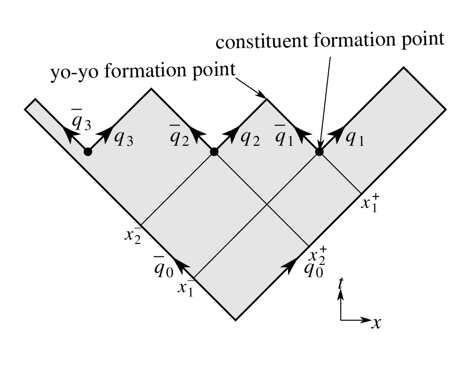
In the Lund string model, space-time coordinates and energy-momentum coordinates for the quarks are directly related via the string tension [169, 170]. Let us consider one-dimensional massless $q\bar{q}$ string in the c.m. frame. If $x_{i}^{\pm}=t_{i}\pm x_{zi}$ denote the light-cone coordinates of the $i$ -th production point, then the light cone momenta $p_{i}^{\pm}=E_{n}\pm p_{zi}$ of the $i$ -th rank hadron which is produced by the energy-momentum fraction $z_{i}$ from ( $i-1$ )-th string $p^{+}_{i}=z_{i}p^{+}_{i-1}$ are fixed by

p_{i}^{+}=\kappa(x_{i-1}^{+}-x_{i}^{+}),\quad p_{i}^{-}=\kappa(x_{i}^{-}-x_{i-1}^{-}),

(122)

with initial value for quark $q_{0}$ moving to the right

x^{+}_{0}={W\over\kappa},\qquad x^{-}_{0}=0,

(123)

where $W$ corresponds to the string initial invariant mass. The probability distribution for the momentum fraction $z_{i}$ is given by the Lund symmetric fragmentation function

f(z)\propto\frac{(1-z)^{a}}{z}\exp\left(-b\frac{(m^{2}+\bm{p}_{\perp}^{2})}{z}\right)\ ,

(124)

where $a$ and $b$ are parameters which have to be fitted to experimental data, and $m$ and $\bm{p}_{\perp}$ denote the mass and transverse momentum of the produced hadron, respectively. This form can be obtained by the condition of the left-right symmetry for the decay of string.

Using the relation $p_{i}^{+}p_{i}^{-}=m_{i\perp}^{2}$ with $m_{i\perp}$ being transverse mass of the $i$ -th hadron, we have the recursion formulae [169]

x_{i}^{+}=(1-z_{i})x^{+}_{i-1},\quad x_{i}^{-}=x^{-}_{i-1}+\left({m_{i\perp}\over\kappa}\right)^{2}{1-z_{i}\over z_{i}}{1\over x^{+}_{i}}.

(125)

Yo-yo formation points where the two $q\bar{q}$ meet for the first time are obtained as

x_{i}^{\mathrm{yo-yo}}=(x_{i-1}^{+},x_{i}^{-}),

(126)

and constituent formation points where $q\bar{q}$ is created

x_{i}^{\mathrm{const}}=(x_{i}^{+},x_{i}^{-}).

(127)

In RQMD [131], the formation points of hadrons are calculated as the average of the two $q\bar{q}$ production point as

x_{i}^{\mathrm{RQMD}}=\left({x_{i}^{+}+x_{i-1}^{+}\over 2},{x_{i}^{-}+x_{i-1}^{-}\over 2}\right).

(128)

Clearly, one can see that

x_{i}^{\mathrm{const}}<x_{i}^{\mathrm{RQMD}}<x_{i}^{\mathrm{yo-yo}}~.

(129)

It is assumed in UrQMD and JAM that the yo-yo formation point is assigned to the space-time point for produced hadrons. The produced hadrons which have the original constituent quarks are allowed to scatter with reduced cross section according to the number of constituent quarks. For example, if baryon has one original constituent quark, cross section during the formation time would be reduced by the factor one-third.

6 Non-Abelian plasmas

Understanding the dynamics of the non-equilibrium system and the process toward the thermalization is a very important outstanding question in high energy heavy ion collisions. In Ref. \citenBMSS, “Bottom-up thermalization” was proposed based on the Boltzmann equation with inelastic processess. Later, full numerical simulations of the Boltzmann equation [146] show that inelastic gluon scatterings are very important processes for thermalization of gluonic systems. It was, however, pointed out that the soft classical color fields may play an important role in the dynamics of thermalization. Specifically, Weibel-like QCD plasma instabilities may develop due to anisotropic distribution of hard plasma particles (partons) [13, 15, 14]. First numerical simulation was done within the hard-loop approximation by solving linearized Vlasov equation in one-dimension [172]. In this analysis, exponential growth of gauge fields due to Abelianization of the field was found. In full 3-dimensional simulations [173, 174], it was found that instabilities grow linearly once the field strength becomes large and non-Abelian self-interactions among gluon fields become nonperturbative in the case of moderate anisotropic momentum distribution. In this case, non-Abelian interactions develop a cascade of energy from soft modes to hards modes [175]. However, in the case of extreme anisotropy [177, 176], energy coming from plasma particles due to Weibel-like instability does not go to the soft mode, instead go back to the hard scale very rapidly which is called “ultraviolet avalanche” in non-Abelian plasmas.

Instabilities of the gluon fields have been also investigated by employing pure classical Yang-Mills equation [178, 179, 180, 181]. It was pointed out [180] that instabilities in the classical Yang-Mills field are the Nielsen-Olsen type instability. Numerical analysis was performed in Ref. \citenBerges:2011sb. In Nielsen-Olsen instability, unstable mode exists at zero momentum, while zero momentum mode is stable in Weibel instability. This is one of the crucial differences between Weibel and Nielsen-Olsen instabilities.

In this section, we review how to solve Wong-Yang-Mills equation based on the technique developed in Ref. \citenDumitru:2006pz below.

6.1 Simulation of non-Abelian plasma

We present numerical method of the classical Vlasov transport equation for gluons with non-Abelian color charge $q^{a}$

p^{\mu}[\partial_{\mu}+gq^{a}F^{a}_{\mu\nu}\partial^{\nu}_{p}+gf_{abc}A^{b}_{\mu}q^{c}\partial_{q^{a}}]f(x,p,q)=0

(130)

where $f(\bm{x},\bm{p},q)$ denotes the single-particle distribution function and $g$ is the gauge coupling. The Vlasov equation is coupled self-consistently to the Yang-Mills equation

D_{\mu}F^{\mu\nu}=J^{\nu}=g\int\frac{d^{3}p}{(2\pi)^{3}}dqqv^{\nu}f(t,\bm{x},\bm{p},q),

(131)

with $v^{\nu}=(1,\bm{p}/p)$ , $D_{\mu}=\partial_{\mu}+igA_{\mu}$ $F_{\mu\nu}=\partial_{\mu}A_{\nu}-\partial_{\nu}A_{\mu}+ig[A_{\mu},A_{\nu}]$ , and $J^{\nu}$ denotes the current generated by plasma particles. This set of equations reproduces the “hard thermal loop” effective theory [183] near equilibrium.

The Vlasov equation can be solved by replacing the one-particle distribution function with many “test particles”:

f(\bm{x},\bm{p},q)=\frac{(2\pi)^{3}}{N_{\mathrm{test}}}\sum_{i}\delta(\bm{x}-\bm{x}_{i}(t))\delta(\bm{p}-\bm{p}_{i}(t))\delta(q-q_{i}(t)),

(132)

where $N_{\mathrm{test}}$ is the number of test particles, and $\bm{x}_{i}(t)$ , $\bm{p}_{i}(t)$ and $q_{i}(t)$ are the coordinate, momentum and the color charge of the test particle. From this assumption, one gets the Wong equation [184] for the $i$ -th “test particle”

\frac{d\bm{x}_{i}}{dt}=\bm{v}_{i},\quad\frac{d\bm{p}_{i}}{dt}=g\,q_{i}^{a}\,\left(\bm{E}^{a}+\bm{v}_{i}\times\bm{B}^{a}\right),\quad\frac{dq_{i}}{dt}=-ig\,v^{\mu}_{i}\,[A_{\mu},q_{i}]

(133)

The time evolution of the Yang-Mills field can be followed by the Hamiltonian method [185] in the temporal gauge. The Hamilton equation of motion for gauge field $A_{i}=A_{i}^{a}t^{a}$ and the color electric field $E_{i}=E_{i}^{a}t^{a}$ under the temporal gauge $A^{0}=0$ is

\frac{dA_{i}}{dt}=E^{i},\qquad\frac{dE^{i}}{dt}=\sum_{j}D_{j}F_{ji}-J^{i},\quad(i,j=x,y,z)

(134)

One may descritize the equation on the lattice size $a$ by introducing the link variable $U_{i}(x)=\exp(iagA_{i}(x))$

	$\displaystyle\dot{U}_{i}(x)$	$\displaystyle=$	$\displaystyle iagE^{i}(x)U_{i}(x),$		(135)
	$\displaystyle\dot{E}^{i}_{a}(x)$	$\displaystyle=$	$\displaystyle\frac{-i}{2a^{3}g}\sum_{j}\mbox{${\rm Tr}$}\left\{t^{a}[U_{ji}(x)-U_{j}^{\dagger}(x-j)U_{ji}(x-j)U_{j}(x-j)]\right\}-J^{i}_{a}$		(136)

where, the plaquette is defined as $U_{\Box}=U_{ij}(x)=U_{i}(x)U_{j}(x+i)U^{\dagger}_{i}(x+j)U^{\dagger}_{j}(x)$ , and $t^{a}=\sigma^{a}$ is the Pauli matrix for SU(2) case. This equation is covariant under the lattice gauge transformation

U_{i}(x)\to V(x)U_{i}(x)V^{\dagger}(x+i),\qquad E^{i}(x)\to V(x)E^{i}(x)V^{\dagger}(x),\qquad

(137)

Typically one uses the time step size of $\Delta t\approx 0.05a$ to ensure energy conservation

H=\sum_{i,x}{a^{3}\over 2}E^{2}_{i}(x)+\sum_{\Box}{1\over 2g^{2}a}(N_{c}-\mbox{${\rm Re}$}\mbox{${\rm Tr}$}U_{\Box})+\frac{1}{N_{\text{test}}}\sum_{j}|\bm{p}_{j}|

(138)

and Gauss law

\sum_{i}\left(E_{i}(x)-U_{i}^{\dagger}(x-i)E_{i}(x-i)U_{i}(x-i)\right)=\rho(x)

(139)

Numerical method has been developed to solve the equations (133) in Ref. \citenHuMullerMoore which is the non-Abelian extension of the nearest-grid-point (NGP) method. In the NGP method, the charge density is obtained by counting the number of particles within a cell. A current $J(x)=Q\delta(t-t_{\text{cross}})/N_{\text{test}}$ is generated only when a particle with the color charge $Q$ crosses a cell boundary from $x$ to $x+i$ at the time $t_{\text{cross}}$ . In order to satisfy the requirement of the lattice covariant continuity equation

\dot{\rho}(x)=\sum_{i}U_{i}^{\dagger}(x-i)J_{i}(x-i)U_{i}(x-i)-J_{i}(x)\ ,

(140)

the color charge must be parallel transported

Q(x+i)=U_{i}^{\dagger}(x)Q(x)U_{i}(x)\ .

(141)

At each time step, an effect of magnetic field, which causes a rotation of momentum and does not change the energy of the particle, on the particle is taken into account. But the magnitude of the momentum can change when it crosses a cell boundary. The final momentum $|\bm{p}_{\mathrm{fin}}|$ after crossing the cell can be fixed by the energy conservation

|\bm{p}_{\mathrm{ini}}|+\frac{N_{\mathrm{test}}}{2}\bm{E}_{\mathrm{ini}}^{2}=|\bm{p}_{\mathrm{fin}}|+\frac{N_{\mathrm{test}}}{2}(\bm{E}_{\mathrm{ini}}-J)^{2}~.

(142)

Substituting $J={Q}/{N_{\mathrm{test}}}$ and when a particle crosses the cell boundary in $x$ -direction, one obtains for new momentum in the $x$ -direction

p_{x}=\sqrt{|\bm{p}_{\mathrm{ini}}|-E_{x,\mathrm{ini}}Q+Q^{2}/(2N_{\mathrm{test}})-p_{\perp}^{2}}~,

(143)

where $|\bm{p}_{\mathrm{fin}}|=\sqrt{p_{x}^{2}+p_{\perp}^{2}}$ is used. As we explained above, because of the current discontinuities introduced in NGP method, large amounts of noise are generated. In order to eliminate this noise, we need a large number of test particle. NGP method was applied in [187, 188, 189] for one-dimensional case in which gauge field is assumed to depend only on one-direction: $\bm{A}(x,y,z)=\bm{A}(z)$ . We call this approximation as 1d-3v simulation because particle velocity has three direction. In 1d-3v case, we can take a very large number of test particle to obtain sufficiently smooth current. However, for full 3d-3v simulation, computational cost may be very expensive due to the larger number of test particle required, and we need improved algorithms.

6.1.1 Particle-in-Cell (PIC) simulations

In Abelian plasmas, particle-in-cell (PIC) method is widely used in which smoothed currents are employed [190, 191, 192] in order to suppress numerical noise. The $m$ -th order shape function (b-spline) $S_{m}$ can be obtained by the convolution of $S_{m-1}$ with the nearest-grid-point weighting function $S_{0}$

S_{m}(x)=\int^{\infty}_{-\infty}S_{0}(x^{\prime})S_{m-1}(x-x^{\prime})dx^{\prime}

(144)

where zero-th-order function is the flat-top function

S_{0}(x)=\left\{\begin{array}[]{ll}1&\mathrm{for}\,|x|\leq\dfrac{1}{2},\\ 0&\mathrm{otherwise}\end{array}\right.

(145)

Commonly used is the first-order function $S_{1}$ which corresponds to linear interpolation

S_{1}(x)=\left\{\begin{array}[]{ll}1-|x|&\mathrm{for}\,|x|\leq 1,\\ 0&\mathrm{otherwise}\end{array}\right.

(146)

The charge density at each lattice site is given by the superposition of a particle,

\rho(i,j,k)=\sum_{\text{particle}}\frac{q}{\Delta x\Delta y\Delta z}S_{m}\left(\frac{x-i}{\Delta x}\right)S_{m}\left(\frac{y-i}{\Delta y}\right)S_{m}\left(\frac{z-i}{\Delta z}\right),

(147)

where $(x,y,z)$ is the coordinate of particle, and $\Delta x$ , $\Delta y$ and $\Delta z$ are the lattice spacing in the $x$ , $y$ and $z$ directions, respectively. However, discrete continuity equation would not necessarily be satisfied on the lattice. One may need to solve Poisson equation to recover Gauss law. More efficient numerical methods that satisfy exactly the lattice continuity equation have been developed [193, 194, 195]. In PIC simulation, the total amount of charge is distributed over its surface, and each charge contributes to the charge density in several cells (8 cells for first order in 3-dimension). In NGP method, current is generated only when a particle crosses the cell boundary, but in PIC, current will be continuously generated in a given time interval which is the amount of charge crossing a cell boundary.

Let us try to construct a current which satisfies the lattice continuity equation. Difference of charge density within a time step $\Delta t$ at a lattice site $(i,j)$ in 2-dimensional case is

		$\displaystyle\rho^{t+\Delta t}(i,j)-\rho^{t}(i,j)$
		$\displaystyle=\sum_{\text{particle}}\frac{q}{\Delta x\Delta y}\left\{S^{m}_{i}(x(t+\Delta t))S^{m}_{i}(y(t+\Delta t))-S^{m}_{i}(x(t))S^{m}_{i}(y(t))\right\}$
		$\displaystyle=\sum_{\text{particle}}\int_{t}^{t+\Delta t}\frac{d}{dt}\left(qS_{i}^{m}(x(t))S_{i}^{m}(y(t))\right)dt\ ,$		(148)

where $S_{i}^{m}(x)=\frac{1}{\Delta x}S_{m}\left(\frac{x-i}{\Delta x}\right)$ . By using the identity for the derivative of $S_{m}$

\frac{dS_{m}(x/\Delta x)}{dx}=\frac{1}{\Delta x}[S_{m-1}(x+\Delta x/2)-S_{m-1}(x-\Delta x/2)]

(149)

which follows from the Eq. (144), one finds that the current defined as

J_{\alpha}(i,j,k)=\frac{1}{\Delta x\Delta y\Delta z}\sum_{\text{particle}}qv_{\alpha}S_{m-1}\left(\frac{x-i-\Delta x/2}{\Delta x}\right)W_{m}\left(\frac{y-j}{\Delta y}\right)W_{m}\left(\frac{z-k}{\Delta z}\right)

(150)

satisfies the lattice continuity equation, where

W_{m}(x)=\int^{t+\Delta t}_{t}S_{m}(x)dt\ .

(151)

We consider a particle moving from $(x_{1},y_{1})$ to $(x_{2},y_{2})$ during a time step $\Delta t$ , i.e., $x_{2}=x_{1}+v_{x}\Delta t,\quad y_{2}=y_{1}+v_{y}\Delta t$ . We also restrict ourselves to the case in which $(x_{2},y_{2})$ belongs to the same lattice site $(i,j)$ . In this case, The explicit form for the first shape-factor corresponding linear smearing case is given by

$\displaystyle\rho(i,j)$	$\displaystyle=$	$\displaystyle\frac{1}{\Delta x\Delta y}(1-x)(1-y),\quad\rho(i,j+1)=\frac{1}{\Delta x\Delta y}x(1-y)~,$
$\displaystyle\rho(i,j)$	$\displaystyle=$	$\displaystyle\frac{1}{\Delta x\Delta y}(1-x)y,\qquad\rho_{y}(i+1,j+1)=\frac{1}{\Delta x\Delta y}xy,$	(152)
$\displaystyle J_{x}(i,j)$	$\displaystyle=$	$\displaystyle\frac{1}{\Delta x\Delta y}F_{x}(1-W_{y}),\qquad J_{x}(i,j+1)=\frac{1}{\Delta x\Delta y}F_{x}W_{y}~,$
$\displaystyle J_{y}(i,j)$	$\displaystyle=$	$\displaystyle\frac{1}{\Delta x\Delta y}F_{y}(1-W_{x}),\qquad J_{y}(i+1,j)=\frac{1}{\Delta x\Delta y}F_{y}W_{x}~,$	(153)

where $x=(x_{1}-i)/\Delta x$ , $y=(y_{1}-j)/\Delta y$ , and $(F_{x},F_{y})\equiv\bm{F}$ represents the charge flux

F_{x}=q\frac{x_{2}-x_{1}}{\Delta t}~,\qquad F_{y}=q\frac{y_{2}-y_{1}}{\Delta t}~.

(154)

$W_{x/y}$ is defined at the midpoint between the starting point $(x_{1},y_{1})$ and the end point $(x_{2},y_{2})$

W_{x}=\frac{x_{1}+x_{2}}{2}-i~,\qquad W_{y}=\frac{y_{1}+y_{2}}{2}-j~.

(155)

We use the ‘Zigzag scheme’ developed in Ref. \citenUmeda in case particle crosses the cell boundary within a time step.

Finally, we note that the electromagnetic forces should be smeared in a similar way when a particle momentum is updated [193]. Consider the time derivative of the total energy:

\frac{dE_{\text{tot}}}{dt}=-\sum_{\text{lattice}}\bm{E}\cdot\bm{J}+\sum_{\text{particles}}q_{i}\,\bm{E}(\bm{x}_{i}(t))\cdot\bm{v}_{i}.

(156)

It is clear that the interpolation function for $\bm{E}$ should be the same as that for $\bm{J}$ in order to achieve good energy conservation in the simulation. The electric field $\bm{E}(\bm{x})$ at the particle position $\bm{x}$ is then obtained from

E_{\alpha}(\bm{x})=\sum_{\text{lattice}}S^{0}_{\alpha}S^{1}_{\beta}S^{1}_{\gamma}E_{\alpha}(i,j,k)~,

(157)

while the magnetic field is given by

B_{\alpha}(\bm{x})=\sum_{\text{lattice}}S^{1}_{\alpha}S^{0}_{\beta}S^{0}_{\gamma}B_{\alpha}(i,j,k)~.

(158)

This is motivated by the relations $\bm{E}=-\nabla A^{0}-\dot{\bm{A}}$ and $\bm{B}=\nabla\times\bm{A}$ .

Next we consider the discretization of the equation Eq. (133) for momentum update. The difference form of the equation is

\frac{\bm{p}(t+\Delta t/2)-\bm{p}(t-\Delta t/2)}{\Delta t}=gq^{a}\left(\bm{E}^{a}(t)+\frac{\bm{p}(t+\Delta t/2)+\bm{p}(t-\Delta t/2)}{2}\times\frac{\bm{B}^{a}(t)}{e(t)}\right)~.

(159)

Equation (159) can be solved by the Buneman-Boris method [191, 190] as follows:

$\displaystyle\bm{p}(t)$	$\displaystyle=$	$\displaystyle\bm{p}(t-\Delta t/2)+\frac{\Delta t}{2}\bm{E}(t),$	(160)
$\displaystyle e(t)$	$\displaystyle=$	$\displaystyle\|\bm{p}(t)\|,$	(161)
$\displaystyle\bm{p}^{\prime}(t)$	$\displaystyle=$	$\displaystyle\bm{p}(t)+\frac{\Delta t}{2}\bm{p}(t)\times\frac{\bm{B}(t)}{e(t)},$	(162)
$\displaystyle\bm{p}_{2}(t)$	$\displaystyle=$	$\displaystyle\bm{p}(t)+\frac{2}{1+(\bm{B}/e(t)\Delta t/2)^{2}}\frac{\Delta t}{2}\bm{p}^{\prime}(t)\times\frac{\bm{B}(t)}{e(t)},$	(163)
$\displaystyle\bm{p}(t+\Delta t/2)$	$\displaystyle=$	$\displaystyle\bm{p}_{2}(t)+\frac{\Delta t}{2}\bm{E}(t),$	(164)

where $\bm{E}\equiv gq^{a}\bm{E}^{a}$ and $\bm{B}\equiv gq^{a}\bm{B}^{a}$ . This scheme is time reversible and the overall momentum integration is accurate to second-order in the time step.

6.2 PIC simulations in non-Abelian gauge theories (CPIC)

An extension of the charge conserved method to the smearing method in the non-Abelian case has been proposed in Ref. \citenDumitru:2006pz in which the current is defined as

	$\displaystyle J_{x}(i,j)$	$\displaystyle=$	$\displaystyle Q\frac{x_{2}-x_{1}}{\Delta t}(1-W_{y}),\qquad J_{x}(i,j+1)=Q_{y}\frac{x_{2}-x_{1}}{\Delta t}W_{y}~,$		(165)
	$\displaystyle J_{y}(i,j)$	$\displaystyle=$	$\displaystyle Q\frac{y_{2}-y_{1}}{\Delta t}(1-W_{x}),\qquad J_{y}(i+1,j)=Q_{x}\frac{y_{2}-y_{1}}{\Delta t}W_{x}~,$		(166)

where we define the parallel transport of the charge in two dimension as

Q_{x}\equiv U_{x}^{\dagger}(i,j)QU_{x}(i,j),\qquad Q_{y}\equiv U_{y}^{\dagger}(i,j)QU_{y}(i,j)~.

(167)

One can easily check that this satisfies the lattice covariant continuity equation,

\dot{\rho}(i,j)=\sum_{x}U^{\dagger}_{x}(i-x)J_{x}(i-x)U_{x}(i-x)-J_{x}(i,j),

(168)

for sites $(i,j),(i+1,j),(i,j+1)$ :

$\displaystyle\dot{\rho}(i,j)$	$\displaystyle=$	$\displaystyle J_{x}(i,j)+J_{y}(i,j),$	(169)
$\displaystyle\dot{\rho}(i+1,j)$	$\displaystyle=$	$\displaystyle U^{\dagger}_{x}(i,j)J_{x}(i,j)U_{x}(i,j)-J_{y}(i+1,j),$	(170)
$\displaystyle\dot{\rho}(i,j+1)$	$\displaystyle=$	$\displaystyle U^{\dagger}_{y}(i,j)J_{y}(i,j)U_{y}(i,j)-J_{x}(i,j+1),$	(171)

Equations (169), (170) and (171) are consistent with the following definitions of the charge densities:

$\displaystyle\rho(i,j)$	$\displaystyle=$	$\displaystyle Q(1-x)(1-y)~,$	(172)
$\displaystyle\rho(i,j+1)$	$\displaystyle=$	$\displaystyle Q_{y}(1-x)y~,$	(173)
$\displaystyle\rho(i+1,j)$	$\displaystyle=$	$\displaystyle Q_{x}x(1-y)~.$	(174)

However, since a particle’s color charge depends on its path, so does $\rho(i+1,j+1)$ and we are not able to calculate it from the charge distribution itself. Rather, we directly employ covariant current conservation to determine the increment of charge at site $(i+1,j+1)$ within the time-step. In this way, we can satisfy Gauss’s law in the non-Abelian case.

Finally, we have to check that $\mbox{${\rm Tr}$}(Q^{2})$ is conserved by this smearing method. This is true when the lattice spacing $a$ is small, as the total charge of a particle is given by

Q_{0}=Q(1-x)(1-y)+Q_{x}x(1-y)+Q_{y}(1-x)y+[a_{p}Q_{xy}+(1-a_{p})Q_{yx}]xy~,

(175)

where the $a_{p}$ depend on the path of a particle and $Q_{xy}=U^{\dagger}_{x}(i,j+1)Q_{y}U_{x}(i,j+1)$ , $Q_{yx}=U^{\dagger}_{y}(i+1,j)Q_{x}U_{y}(i+1,j)$ . If we require that $\mbox{${\rm Tr}$}(Q_{0}^{2})$ be constant, then the cross terms, for example $\mbox{${\rm Tr}$}(QQ_{x})$ , have to vanish. This is true when $a$ is small, because $\mbox{${\rm Tr}$}(Q[A,Q])=0$ :

\mbox{${\rm Tr}$}(QQ_{x})=\mbox{${\rm Tr}$}(Q(Q+iga[A_{x},Q]+{\cal O}(a^{2})))=\mbox{${\rm Tr}$}(Q^{2})+{\cal O}(a^{2}).

(176)

Therefore, the magnitude of the color charges is conserved for small lattice size $a$ in our method.

7 Summary

We have reviewed recent progress on the development of dynamical models in heavy ion collisions. Our emphasis was put on the technical aspects of the models. Initial particle production processes are obtained by the CGC framework based on the $k_{T}$ factrization formula. Vlasov simulation of non-Abelian plasma can be followed by the non-Abelian extension of particle-in-cell method. In the locally thermailzed stage, relativistic hydrodynamics can be used to describe space-time evolution of matter. Energy loss of energetic partons in the expanding fluid elements is necessary for the consistent description of the jet quenching as well as two-particle correlations. Finally, effects of final state interactions during the hadronic gas state are also important for the realistic simulation of heavy ion collisions.

Recently there have been made significant progresses for theoretical approaches. Viscous hydrodynamic simulations have been performed by many groups [196] to extract transport coefficients such as a ratio of shear viscosity to entropy density.

Numerical solutions of the classical Yang-Mills equations are first employed for the initial condition of event-by-event hydrodynamical simulations [75]. JIMWLK renormalization group evolution equation was used as initial conditions for the classical Yang-Mills equation [197] in order to incorporate the rapidity evolution of the probability distribution for Wilson lines. This approach may give an important initial condition for hydrodynamic simulations. SU(2) plasma simulations of Boltzmann-Vlasov equation including both collision term for hard particles and soft interaction by classical Yang-Mills fields are performed in Refs. \citenDumitru:2007rp,Schenke:2008gg,Schenke:2008pm,Schenke:2009jy. It was demonstrated that results are independent of the choice of separation scale between hard and soft modes. Inclusion of inelastic process is important for the jet energy loss in the early stages of heavy ion collision before thermalization.

One of the outstanding problems in high energy collisions at RHIC and LHC is the missing understanding of non-equilibrium dynamics in the early stages. Recent progress on the investigations how non-Abelian plasmas or Glasma approach equilibrium state in heavy ion collisions can be found, e.g., in Refs. \citenGelis:2007pw,Dusling:2010rm,Kurkela:2011ti,Hatta:2011ky. Non-equilibrium simulations for these approaches will provide insight into the mechanism of thermalization in heavy ion collisions.

Acknowledgments

The authors acknowledges the fruitful collaboration with A. Dumitru, H.-J. Drescher, P. Huovinen, and M. Strickland. The work was partly supported by Grant-in-Aid for Scientific Research Nos. 22740151 and 22340052. The work of Y.N. was supported by Grant-in-Aid for Scientific Research No. 20540276.

References

[1] K. Yagi, T. Hatsuda and Y. Miake, Quark-gluon plasma: From big bang to little bang, (Cambridge, 2005).
[2] M. Gyulassy, arXiv:nucl-th/0403032.
[3] T. D. Lee, Nucl. Phys. A 750 (2005), 1; M. Gyulassy, L. McLerran, Nucl. Phys. A 750 (2005), 30; E. V. Shuryak, Nucl. Phys. A 750 (2005), 64.
[4] E. Iancu, A. Leonidov and L. McLerran, arXiv:hep-ph/0202270; E. Iancu and R. Venugopalan, Quark Gluon Plasma 3 (QGP3):249-363,2004. Eds. R.C. Hwa and X.N.Wang, World Scientific (2004), arXiv:hep-ph/0303204; F. Gelis, E. Iancu, J. Jalilian-Marian and R. Venugopalan, Ann. Rev. Nucl. Part. Sci. 60 (2010), 463.
[5] G. Gatoff, A. K. Kerman and T. Matsui, Phys. Rev. D 36 (1987), 114.
[6] T. Lappi and L. McLerran, Nucl. Phys. A 772 (2006), 200.
[7] A. Dumitru, F. Gelis, L. McLerran and R. Venugopalan, Nucl. Phys. A 810 (2008), 91.
[8] K. Dusling, F. Gelis, T. Lappi and R. Venugopalan, Nucl. Phys. A 836 (2010), 159.
[9] A. Dumitru, K. Dusling, F. Gelis, J. Jalilian-Marian, T. Lappi and R. Venugopalan, Phys. Lett. B 697 (2011), 21.
[10] B. I. Abelev et al. [STAR Collaboration], Phys. Rev. C 80 (2009), 064912.
[11] B. Alver et al. [PHOBOS Collaboration], Phys. Rev. Lett. 104 (2010), 062301.
[12] V. Khachatryan et al. [CMS Collaboration], JHEP 1009 (2010), 091.
[13] S. Mrowczynski, Phys. Lett. B 214 (1988), 587; Phys. Lett. B 314 (1993), 118; Phys. Rev. C 49 (1994), 2191.
[14] P. Romatschke and M. Strickland, Phys. Rev. D 68 (2003), 036004; Phys. Rev. D 70 (2004), 116006; S. Mrowczynski, A. Rebhan and M. Strickland, Phys. Rev. D 70 (2004), 025004.
[15] P. Arnold, J. Lenaghan, and G. D. Moore, JHEP 0308 (2003), 002; P. B. Arnold and J. Lenaghan, Phys. Rev. D 70 (2004), 114007; P. B. Arnold, J. Lenaghan, G. D. Moore and L. G. Yaffe, Phys. Rev. Lett. 94 (2005), 072302.
[16] F. Gelis, A. M. Stasto and R. Venugopalan, Eur. Phys. J. C 48 (2006), 489.
[17] J. L. Albacete, Phys. Rev. Lett. 99 (2007), 262301.
[18] E. Levin and A. H. Rezaeian, Phys. Rev. D 82 (2010), 014022; Phys. Rev. D 82 (2010), 054003; Phys. Rev. D 83 (2011), 114001.
[19] P. Tribedy and R. Venugopalan, Nucl. Phys. A 850 (2011), 136 [Erratum-ibid. A 859 (2011), 185]; arXiv:1112.2445 [hep-ph].
[20] D. Kharzeev and M. Nardi, Phys. Lett. B507 (2001), 121; D. Kharzeev and E. Levin, ibid. B523 (2001), 79; D. Kharzeev, E. Levin, and M. Nardi, Phys. Rev. C 71 (2005), 054903; Nucl. Phys. A730 (2004), 448.
[21] A. Adil, H. J. Drescher, A. Dumitru, A. Hayashigaki, and Y. Nara, Phys. Rev. C 74 (2006), 044905.
[22] H. J. Drescher and Y. Nara, Phys. Rev. C 75 (2007), 034905; 76 (2007), 041903(R).
[23] A. Dumitru, D. E. Kharzeev, E. M. Levin and Y. Nara, arXiv:1111.3031 [hep-ph].
[24] J. L. Albacete and A. Dumitru, 1011.5161[hep-ph]; http://physics.baruch.cuny.edu/node/people/adumitru/res_cgc
[25] A. Krasnitz and R. Venugopalan, Nucl. Phys. B 557 (1999), 237; Phys. Rev. Lett. 84 (2000), 4309; ibid. 86 (2001), 1717; A. Krasnitz, Y. Nara, and R. Venugopalan, Phys. Rev. Lett. 87 (2001), 192302; Nucl. Phys. A 717 (2003), 268.
[26] T. Lappi, Phys. Rev. C 67 (2003), 054903; Phys. Rev. C 70 (2004), 054905.
[27] A. Krasnitz, Y. Nara, and R. Venugopalan, Nucl. Phys. A 727 (2003), 427.
[28] A. Krasnitz, Y. Nara, and R. Venugopalan, Phys. Lett. B 554 (2003), 21.
[29] P. F. Kolb, P. Huovinen, U. W. Heinz and H. Heiselberg, Phys. Lett. B 500 (2001), 232.
[30] P. Huovinen, P. F. Kolb, U. W. Heinz, P. V. Ruuskanen and S. A. Voloshin, Phys. Lett. B 503 (2001), 58.
[31] D. Teaney, J. Lauret and E. V. Shuryak, Phys. Rev. Lett. 86 (2001), 4783; arXiv:nucl-th/0110037.
[32] T. Hirano, Phys. Rev. C 65 (2002), 011901.
[33] T. Hirano, K. Tsuda, Phys. Rev. C 66 (2002), 054905.
[34] J. Y. Ollitrault, Phys. Rev. D 46 (1992), 229.
[35] C. Adler et al. [STAR Collaboration], Phys. Rev. Lett. 87 (2001), 182301; Phys. Rev. C 66 (2002), 034904; J. Adams et al. [STAR Collaboration], Phys. Rev. Lett. 92 (2001), 052302; Phys. Rev. C 72 (2005), 014904; B. I. Abelev et al. [STAR Collaboration], Phys. Rev. C 77 (2008), 054901.
[36] K. Adcox et al. [PHENIX Collaboration], Phys. Rev. Lett. 89 (2002), 212301; S.S. Adler et al. [PHENIX Collaboration] Phys. Rev. Lett. 91 (2003), 182301; Phys. Rev. Lett. 94 (2005), 232302; A. Adare et al. [PHENIX Collaboration], Phys. Rev. Lett. 98 (2007), 162301.
[37] B. B. Back et al. [PHOBOS Collaboration], Phys. Rev. Lett. 89 (2002), 222301; Phys. Rev. Lett. 94 (2005), 122303; B. Alver et al. [PHOBOS Collaboration], Phys. Rev. Lett. 98 (2007), 242302.
[38] KAamodt et al. [The ALICE Collaboration], Phys. Rev. Lett. 105 (2010), 252302.
[39] G. Aad et al. [ATLAS Collaboration], Phys. Lett. B 707 (2012), 330.
[40] J. Velkovska [CMS Collaboration], J. Phys. G 38 (2011), 124011.
[41] http://www.bnl.gov/bnlweb/pubaf/pr/PR_display.asp?prID=05-38
[42] T. Hirano and M. Gyulassy, Nucl. Phys. A 769 (2006), 71.
[43] S. A. Bass, A. Dumitru, M. Bleicher, L. Bravina, E. Zabrodin, H. Stoecker and W. Greiner, Phys. Rev. C 60 (1999), 021902; S. A. Bass and A. Dumitru, Phys. Rev. C 61 (2000), 064909.
[44] T. Hirano, U. W. Heinz, D. Kharzeev, R. Lacey, Y. Nara, Phys. Lett. B 636 (2006), 299.
[45] C. Nonaka and S. A. Bass, Phys. Rev. C 75 (2007), 014902.
[46] K. Werner, I. .Karpenko, T. Pierog, M. Bleicher and K. Mikhailov, Phys. Rev. C 82 (2010), 044904.
[47] R. J. Fries, V. Greco and P. Sorensen, Ann. Rev. Nucl. Part. Sci. 58 (2008), 177.
[48] U. A. Wiedemann, arXiv:0908.2306 [hep-ph].
[49] D. d’Enterria, arXiv:0902.2011 [nucl-ex].
[50] A. Majumder and M. Van Leeuwen, Prog. Part. Nucl. Phys. A 66 (2011), 41.
[51] R. J. Fries and C. Nonaka, Prog. Part. Nucl. Phys. 66 (2011), 607.
[52] K. Adcox et al. [PHENIX Collaboration], Phys. Rev. Lett. 88 (2002), 022301; S. S. Adler et al. [PHENIX Collaboration], Phys. Rev. Lett. 91 (2003), 072301.
[53] C. Adler et al. [STAR Collaboration], Phys. Rev. Lett. 89 (2002), 202301; J. Adams et al. [STAR Collaboration], Phys. Rev. Lett. 91 (2003), 172302.
[54] K. Aamodt et al. [ALICE Collaboration], Phys. Lett. B 696 (2011), 30; G. Aad et al. [ATLAS Collaboration], Phys. Rev. Lett. 105 (2010), 252303; S. Chatrchyan et al. [CMS Collaboration], Phys. Rev. C 84 (2011), 024906.
[55] C. Adler et al. [STAR Collaboration], Phys. Rev. Lett. 90 (2003), 082302.
[56] B. B. Back et al. [PHOBOS Collaboration] Phys. Rev. Lett. 91 (2003), 072302; S. S. Adler et al. [PHENIX Collaboration], Phys. Rev. Lett. 91 (2003), 072303; J. Adams et al. [STAR Collaboration] Phys. Rev. Lett. 91 (2003), 072304; I. Arsene et al. [BRAHMS Collaboration], Phys. Rev. Lett. 91 (2003), 072305.
[57] T. Hirano and Y. Nara, Phys. Rev. C 66 (2002), 041901; Phys. Rev. C 69 (2004), 034908.
[58] T. Hirano and Y. Nara, Phys. Rev. Lett. 91 (2003), 082301.
[59] T. Renk, J. Ruppert, C. Nonaka and S. A. Bass, Phys. Rev. C 75 (2007), 031902.
[60] S. A. Bass, C. Gale, A. Majumder, C. Nonaka, G. Y. Qin, T. Renk and J. Ruppert, Phys. Rev. C 79 (2009), 024901.
[61] B. Schenke, C. Gale and S. Jeon, Phys. Rev. C 80 (2009), 054913.
[62] A. Adare et al. [PHENIX Collaboration], Phys. Rev. Lett. 107 (2011), 252301.
[63] C. A. Loizides et al. [ALICE Collaboration], Phys. Rev. Lett. 107 (2011), 032301.
[64] G. Aad et al. [ATLAS Collaboration], arXiv:1203.3087 [hep-ex].
[65] B. Alver and G. Roland, Phys. Rev. C 81 (2010), 054905 [Erratum-ibid. C 82 (2010), 039903].
[66] R. Andrade, F. Grassi, Y. Hama, T. Kodama and O. Socolowski, Jr., Phys. Rev. Lett. 97 (2006), 202302.
[67] B. H. Alver, C. Gombeaud, M. Luzum and J. Y. Ollitrault, Phys. Rev. C 82 (2010), 034913.
[68] H. Petersen, G. Y. Qin, S. A. Bass and B. Muller, Phys. Rev. C 82 (2010), 041901.
[69] G. -Y. Qin, H. Petersen, S. A. Bass, B. Muller, Phys. Rev. C82 (2010), 064903.
[70] B. Schenke, S. Jeon and C. Gale, Phys. Rev. Lett. 106 (2011), 042301.
[71] Z. Qiu, U. W. Heinz, Phys. Rev. C84 (2011), 024911.
[72] F. Gelis, T. Lappi and L. McLerran, Nucl. Phys. A 828 (2009), 149.
[73] A. Dumitru and Y. Nara, arXiv:1201.6382 [nucl-th].
[74] C. Flensburg, arXiv:1108.4862 [nucl-th].
[75] B. Schenke, P. Tribedy and R. Venugopalan, arXiv:1202.6646 [nucl-th].
[76] M. Alvioli, H. J. Drescher and M. Strikman, Phys. Lett. B 680 (2009), 225.
[77] M. Alvioli, H. Holopainen, K. J. Eskola and M. Strikman, Phys. Rev. C 85 (2012), 034902.
[78] T. Hirano, Y. Nara, Nucl. Phys. A743 (2004), 305.
[79] M. Cheng et al., Phys. Rev. D 77 (2008), 014511.
[80] A. Bazavov et al., Phys. Rev. D 80 (2009), 014504.
[81] S. Borsanyi, G. Endrodi, Z. Fodor, A. Jakovac, S. D. Katz, S. Krieg, C. Ratti and K. K. Szabo, JHEP 1011 (2010), 077.
[82] T. Umeda et al. [WHOT-QCD Collaboration], arXiv:1202.4719 [hep-lat].
[83] P. Huovinen, P. Petreczky, Nucl. Phys. A 837 (2010), 26.
[84] https://wiki.bnl.gov/hhic/index.php/Lattice_calculatons_of_Equation_of_State and https://wiki.bnl.gov/TECHQM/index.php/QCD_Equation_of_State
[85] F. Cooper, G. Frye, Phys. Rev. D10 (1974), 186.
[86] L. Levkova, arXiv:1201.1516 [hep-lat].
[87] D. Teaney, nucl-th/0204023.
[88] P. F. Kolb and R. Rapp, Phys. Rev. C 67 (2003), 044903.
[89] P. Huovinen, Eur. Phys. J. A 37 (2008), 121.
[90] W. -L. Qian, R. Andrade, F. Grassi, Y. Hama and T. Kodama, arXiv:0709.0845 [nucl-th].
[91] P. Colella and P. R. Woodward, J. Comput. Phys. 54 (1984), 174.
[92] T. Hirano, Phys. Rev. Lett. 86 (2001), 2754; T. Hirano, K. Tsuda and K. Kajimoto, nucl-th/0011087.
[93] V. Schneider, U. Katscher, D. H. Rischke, B. Waldhauser, J. A. Maruhn and C. D. Munz, J. Comput. Phys. 105 (1993), 92; D. H. Rischke, S. Bernard and J. A. Maruhn, Nucl. Phys. A 595 (1995), 346; D. H. Rischke, Y. Pursun and J. A. Maruhn, Nucl. Phys. A 595 (1995), 383 [Erratum-ibid. A 596 (1996), 717].
[94] M. L. Miller, K. Reygers, S. J. Sanders and P. Steinberg, Ann. Rev. Nucl. Part. Sci. 57 (2007), 205.
[95] W. Broniowski, M. Rybczynski and P. Bozek, Comput. Phys. Commun. 180 (2009), 69.
[96] B. Alver, M. Baker, C. Loizides and P. Steinberg, arXiv:0805.4411 [nucl-ex].
[97] R. M. Barnett et al., Phys. Rev. D 54 (1996), 1.
[98] G. A. Schuler and T. Sjostrand, Nucl. Phys. B 407 (1993), 539; Phys. Rev. D 49 (1994), 2257.
[99] T. Sjostrand, S. Mrenna and P. Z. Skands, JHEP 0605 (2006), 026.
[100] H. De Vries, C. W. De Jager, and C. De Vries, Atom. Data Nucl. Data Tabl. 36 (1987), 495.
[101] T. Hirano and Y. Nara, Phys. Rev. C 79 (2009), 064904.
[102] B.B. Back et al. [PHOBOS Collaboration], Phys. Rev. C 65 (2002), 061901.
[103] T. Hirano, P. Huovinen and Y. Nara, Phys. Rev. C 84 (2011), 011901.
[104] K. Aamodt et al. [ALICE Collaboration], Phys. Rev. Lett. 106 (2011), 032301; Phys. Rev. Lett. 106 (2011), 032301.
[105] K. Aamodt et al. [ALICE Collaboration], Eur. Phys. J. C 68 (2010), 89.
[106] K. Golec-Biernat and M. Wusthoff, Phys. Rev. D 59 (1999), 014017; 60 (1999), 114023.
[107] J. L. Albacete and Y. V. Kovchegov, Phys. Rev. D 75 (2007), 125021.
[108] J. L. Albacete, N. Armesto, J. G. Milhano, and C. A. Salgado, Phys. Rev. D 80 (2009), 034031.
[109] J. L. Albacete, N. Armesto, J. G. Milhano, P. Quiroga Arias and C. A. Salgado, arXiv:1012.4408 [hep-ph].
[110] J. L. Albacete and C. Marquet, Phys. Lett. B 687 (2010), 174; Phys. Rev. Lett. 105 (2010), 162301.
[111] J. Jalilian-Marian and A. H. Rezaeian, Phys. Rev. D 85 (2012), 014017.
[112] J. L. Albacete, A. Dumitru and Y. Nara, J. Phys. Conf. Ser. 316 (2011), 012011.
[113] Y. Nara, arXiv:1110.2847 [nucl-th].
[114] U. Heinz and J. S. Moreland, Phys. Rev. C 84 (2011), 054905.
[115] R. Baier, Y. L. Dokshitzer, A. H. Mueller, S. Peigne and D. Schiff, Nucl. Phys. B 483 (1997), 291; R. Baier, Y. L. Dokshitzer, A. H. Mueller and D. Schiff, Nucl. Phys. B 531 (1998), 403; B. G. Zakharov, JETP Lett. 65 (1997), 615.
[116] M. Gyulassy, P. Levai and I. Vitev, Nucl. Phys. B 571 (2000), 197; Phys. Rev. Lett. 85 (2000), 5535; Nucl. Phys. B 594 (2001), 371.
[117] U. A. Wiedemann, Nucl. Phys. B 588 (2000), 303; C. A. Salgado and U. A. Wiedemann, Phys. Rev. D 68 (2003), 014008; N. Armesto, C. A. Salgado and U. A. Wiedemann, Phys. Rev. D 69 (2004), 114003.
[118] X. -f. Guo and X. -N. Wang, Phys. Rev. Lett. 85 (2000), 3591; X. -N. Wang and X. -f. Guo, Nucl. Phys. A 696 (2001), 788; A. Majumder, Phys. Rev. D 85 (2012), 014023.
[119] P. B. Arnold, G. D. Moore and L. G. Yaffe, JHEP 0112 (2001), 009; JHEP 0112 (2001), 009.
[120] N. Armesto, B. Cole, C. Gale, W. A. Horowitz, P. Jacobs, S. Jeon, M. van Leeuwen and A. Majumder et al., arXiv:1106.1106 [hep-ph].
[121] M. Gyulassy, I. Vitev, X. -N. Wang and P. Huovinen, Phys. Lett. B 526 (2002), 301.
[122] T. Sjöstrand, Comp. Phys. Comm. 82 (1994), 74;
http://www.thep.lu.se/tf2/staff/torbjorn/Pythia.html.
[123] T. Hirano and Y. Nara, Phys. Rev. Lett. 91 (2003), 082301; Phys. Rev. C 69 (2004), 034908; Phys. Rev. C 68 (2003), 064902.
[124] R. Baier, Nucl. Phys. A 715 (2003), 209.
[125] A. Majumder, arXiv:1202.5295 [nucl-th].
[126] J. Cugnon, Phys. Rev. C 22 (1980), 1885.
[127] J. Cugnon, T. Mizutani and J. Vandermeulen, Nucl. Phys. A 352 (1981), 505.
[128] T. Kodama, S. B. Duarte, K. C. Chung, R. Donangelo and R. A. M. Nazareth, Phys. Rev. C 29 (1984), 2146.
[129] G. F. Bertsch and S. Das Gupta, Phys. Rept. 160 (1988), 189.
[130] H. Sorge, H. Stöcker and W. Greiner, Annals Phys. 192, 266, (1989); H. Sorge, A. von Keitz, R. Mattiello, H. Stöcker and W. Greiner, Z. Phys. C 47 (1990), 629; H. Sorge, R. Mattiello, A. Jahns, H. Stoecker and W. Greiner, Phys. Lett. B 271 (1991), 37; H. Sorge, L. Winckelmann, H. Stöcker and W. Greiner, Z. Phys. C 59 (1993), 85.
[131] H. Sorge, Phys. Rev. C 52 (1995), 3291.
[132] N. S. Amelin and L. V. Bravina, Sov. J. Nucl. Phys. 51 (1990), 133 [Yad. Fiz. 51 (1990), 211]; N. S. Amelin, K. K. Gudima and V. D. Toneev, Sov. J. Nucl. Phys. 51 (1990), 1093 [Yad. Fiz. 51 (1990), 1730]; L. Bravina, L.P. Csernai, P. Levai, and D. Strottman, Phys. Rev. C 51 (1994), 2161.
[133] Y. Pang, T. J. Schlagel and S. H. Kahana, Phys. Rev. Lett. 68 (1992), 2743.
[134] B. A. Li and C. M. Ko, Phys. Rev. C 52 (1995), 2037.
[135] L.A. Winckelmann, et al. Nucl. Phys. A610 (1996), 116c; S.A. Bass, et al. Prog. Part. Nucl. Phys. 41 (1998), 225; M Bleicher, et al. J. Phys. G25 (1999), 1859.
[136] Y. Nara, N. Otuka, A. Ohnishi, K. Niita, S. Chiba, Phys. Rev. C 61 (2000), 024901; http://quark.phy.bnl.gov/~ynara/jam/
[137] M. Isse, A. Ohnishi, N. Otuka, P. K. Sahu and Y. Nara, Phys. Rev. C 72 (2005), 064908.
[138] W. Cassing and E. L. Bratkovskaya, Phys. Rept. 308 (1999), 65.
[139] O. Buss, T. Gaitanos, K. Gallmeister, H. van Hees, M. Kaskulov, O. Lalakulich, A. B. Larionov and T. Leitner et al., Phys. Rept. 512 (2012), 1.
[140] K. Geiger and B. Müller,Nucl. Phys. B 369 (1992), 600; K. Geiger, Phys. Rep. 258 (1995), 238; Comp. Phys. Comm. 104 (1997), 70.
[141] T. Renk, S. A. Bass and D. K. Srivastava, Phys. Lett. B 632 (2006), 632.
[142] S. A. Bass, B. Muller and D. K. Srivastava, Phys. Lett. B 551 (2003), 277.
[143] B. Zhang, Comput. Phys. Commun. 109 (1998), 193.
[144] D. Molnar and M. Gyulassy, Phys. Rev. C 62 (2000), 054907.
[145] S. Cheng et al., Phys. Rev. C 65 (2002), 024901.
[146] Z. Xu and C. Greiner, Phys. Rev. C 71 (2005), 064901.
[147] D. Molnar and M. Gyulassy, Nucl. Phys. A 697 (2002), 495 [Erratum-ibid. A 703 (2002), 893].
[148] E. Shuryak and L. Xiong, Phys. Rev. C49 (1994), 2241; T. S. Biro, E. van Doorn, B. Müller, M. H. Thoma and X.-N. Wang, Phys. Rev. C 48 (1993), 1275; S. M. Wong, Nucl. Phys. A 607 (1996), 442; R. Baier, A. H. Mueller, D. Schiff and D. T. Son, Phys. Lett. B 502 (2001), 51.
[149] S. M. Wong, Phys. Rev. C 54 (1996), 2588.
[150] Y. Nara, S. E. Vance and P. Csizmadia, Phys. Lett. B 531 (2002), 209.
[151] Z. W. Lin, C. M. Ko, B. A. Li, B. Zhang and S. Pal, Phys. Rev. C 72 (2005), 064901.
[152] W. Cassing and E. L. Bratkovskaya, Nucl. Phys. A 831 (2009), 215; E. L. Bratkovskaya, W. Cassing, V. P. Konchakovski and O. Linnyk, Nucl. Phys. A 856 (2011), 162.
[153] B. Zhang and Y. Pang, Phys. Rev. C 56 (1997), 2185.
[154] G. Wolf, G. Batko, W. Cassing, U. Mosel, K. Niita and M. Schaefer, Nucl. Phys. A 517 (1990), 615.
[155] G. Kortemeyer, W. Bauer, K. Haglin, J. Murray and S. Pratt, Phys. Rev. C 52 (1995), 2714.
[156] G. Welke, R. Malfliet, C. Gregoire, M. Prakash and E. Suraud, Phys. Rev. C 40 (1989), 2611.
[157] A. Lang, H. Babovsky, W. Cassing, U. Mosel, H-G. Reusch, and K. Weber, J. Comp. Phys. 106 (1993), 391.
[158] P. Danielewicz and G. F. Bertsch, Nucl. Phys. A 533 (1991), 712.
[159] A. Bialas, M. Gyulassy, Nucl. Phys. A 291 (1987), 793.
[160] S. Teis, W. Cassing, M. Effenberger, A. Hombach, U. Mosel and G. Wolf, Z. Phys. A 356 (1997), 421.
[161] Gy.Wolf, W.Cassing, U.Mosel, Nucl. Phys. A 552 (1993), 549.
[162] Bao-An Li, Nucl. Phys. A 552 (1993), 605.
[163] G. E. Brown, C. M. Ko, Z. G. Wu and L. H. Xia, Phys. Rev. C 43 (1991), 1881.
[164] T. Hirano, U. W. Heinz, D. Kharzeev, R. Lacey, Y. Nara, Phys. Rev. C77 (2008), 044909.
[165] X. N. Wang and M. Gyulassy, Phys. Rev. D 44 (1991), 3501; X. N. Wang, Phys. Rep. 280 (1997), 287; X. N. Wang and M. Gyulassy, Comp. Phys. Comm. 83 (1994), 307; http://www-nsdth.lbl.gov/~xnwang/hijing/.
[166] B. Andersson, G. Gustafson and H. Pi, Z. Phys. C 57 (1993), 485; H. Pi, Comp. Phys. Comm. 71 (1992), 173.
[167] A. Capella, U. Sukhatme, C.-I. Tan and J. Tran Thanh Van, Phys. Rep. 236 (1994), 225.
[168] K. Werner, Z. Phys. C 42 (1989), 85; Phys. Rep. 232 (1993), 87.
[169] B. Andersson, G. Gustafson, G. Ingelman and T. Sjöstrand, Phys. Pep. 97 (1983), 31; B. Andersson, The Lund Model, (Cambridge, 2005).
[170] T. Sjöstrand, Nucl. Phys. B 248 (1984), 469.
[171] R. Baier, A. H. Mueller, D. Schiff, and D. T. Son, Phys. Lett. B 502 (2001), 51.
[172] A. Rebhan, P. Romatschke and M. Strickland, Phys. Rev. Lett. 94 (2005), 102303.
[173] P. Arnold, G. D. Moore and L. G. Yaffe, Phys. Rev. D 72 (2005), 054003; A. Rebhan, P. Romatschke and M. Strickland, JHEP 0509 (2005), 041.
[174] A. Rebhan, P. Romatschke and M. Strickland, JHEP 0509 (2005), 041.
[175] P. Arnold and G. D. Moore, Phys. Rev. D 73 (2006), 025006; Phys. Rev. D 76 (2007), 045009.
[176] D. Bodeker and K. Rummukainen, JHEP 0707 (2007), 022.
[177] A. Dumitru, Y. Nara and M. Strickland, Phys. Rev. D 75 (2007), 025016.
[178] P. Romatschke and R. Venugopalan, Phys. Rev. Lett. 96 (2006), 062302; Phys. Rev. D 74 (2006), 045011.
[179] K. Fukushima, F. Gelis and L. McLerran, Nucl. Phys. A 786 (2007), 107; K. Fukushima, Phys. Rev. C 76 (2007), 021902 [Elrratum-ibid. C 77 (2007), 029901]; K. Fukushima and F. Gelis, Nucl. Phys. A 874 (2012), 108.
[180] A. Iwazaki, Phys. Rev. C 77 (2008), 034907; H. Fujii and K. Itakura, Nucl. Phys. A 809 (2008), 88; H. Fujii, K. Itakura and A. Iwazaki, Nucl. Phys. A 828 (2009), 178.
[181] J. Berges, S. Scheffler and D. Sexty, Phys. Rev. D 77 (2008), 034504.
[182] J. Berges, S. Scheffler, S. Schlichting and D. Sexty, Phys. Rev. D 85 (2012) 034507.
[183] P. F. Kelly, Q. Liu, C. Lucchesi and C. Manuel, Phys. Rev. Lett. 72 (1994), 3461; Phys. Rev. D 50 (1994), 4209; J. P. Blaizot and E. Iancu, Nucl. Phys. B 557 (1999), 183; Phys. Rept. 359 (2002), 355.
[184] S. K. Wong, Nuovo Cim. A 65 (1970), 689; H. T. Elze and U. W. Heinz, Phys. Rept. 183 (1989), 81; D. F. Litim and C. Manuel, Phys. Rept. 364 (2002), 451.
[185] J. Ambjørn, T. Askgaard, H. Porter, and M. E. Shaposhnikov, Nucl. Phys. B 353 (1991), 346.
[186] C. R. Hu and B. Müller, Phys. Lett. B 409 (1997), 377; G. D. Moore, C. R. Hu and B. Müller, Phys. Rev. D 58 (1998), 045001.
[187] A. Dumitru and Y. Nara, Phys. Lett. B 621 (2005), 89.
[188] A. Dumitru and Y. Nara, Eur. Phys. J. A 29 (2006), 65.
[189] Y. Nara, Nucl. Phys. A 774 (2006), 783.
[190] C. K. Birdsall and A. Langdon, Plasma Physics via Computer Simulation (McGraw-Hill, New York, 1985).
[191] R. W. Hockney and J. W. Eastwood, Computer Simulation Using Particles (McGraw-Hill, New York, 1988).
[192] Computer Space Plasma Physics: Simulation Techniques and Software, Edited by H. Matsumoto and Y. Omura, http://www.terrapub.co.jp/e-library/cspp/index.html
[193] J. W. Eastwood, Comput. Phys. Commun. 64 (1991), 252; J. W. Eastwood, W. Arter, N. J. Brealey, and R. Hockney, Comput. Phys. Commun. 87 (1995), 155.
[194] O. Buneman and J. Villasenor, Comput. Phys. Commun. 69 (1992), 306; T. Z. Esirkepov, Comput. Phys. Commun. 135 (2001), 144.
[195] T. Umeda, Y. Omura, T. Tominaga, and H. Matsumoto, Comput. Phys. Commun. 156 (2003), 73.
[196] A. Muronga, Phys. Rev. Lett. 88 (2003), 062302 [Erratum-ibid. 89 (2002), 159901]; Phys. Rev. C 69 (2004), 034903; Phys. Rev. C 76 (2007), 014909; Phys. Rev. C 76 (2007), 014910; U. W. Heinz, H. Song and A. K. Chaudhuri, Phys. Rev. C 73 (2006), 034904; H. Song and U. W. Heinz, Phys. Lett. B 658 (2008), 279; Phys. Rev. C 77 (2008), 064901; Phys. Rev. C 78 (2008), 024902; A. K. Chaudhuri, arXiv:0704.0134 [nucl-th]; arXiv:0708.1252 [nucl-th]; arXiv:0801.3180 [nucl-th]; Phys. Lett. B 672 (2009), 126; R. Baier, P. Romatschke and U. A. Wiedemann, Phys. Rev. C 73 (2006), 064903; Nucl. Phys. A 782 (2007), 313; R. Baier and P. Romatschke, Eur. Phys. J. C 51 (2007), 677; P. Romatschke and U. Romatschke, Phys. Rev. Lett. 99 (2007), 172301; M. Luzum and P. Romatschke, Phys. Rev. C 78 (2008), 034915; arXiv:0901.4588 [nucl-th]; K. Dusling and D. Teaney, Phys. Rev. C 77 (2008), 034905; P. Huovinen and D. Molnar, Phys. Rev. C 79 (2009), 014906; K. Paech and S. Pratt, Phys. Rev. C 74 (2006), 014901; T. Koide, G. S. Denicol, Ph. Mota, and T. Kodama, Phys. Rev. C 75 (2007), 034909; G. S. Denicol, T. Kodama, T. Koide, and Ph. Mota, C 78 (2008), 034901; arXiv:0903.3595 [hep-ph]; G. Torrieri and I. Mishustin, Phys. Rev. C 78 (2008), 021901; R. J. Fries, B. Muller, and A. Schafer, Phys. Rev. C 78 (2008), 034913; A. Monnai and T. Hirano, Phys. Lett. B 703 (2011), 583.
[197] T. Lappi, Phys. Lett. B 703 (2011), 325.
[198] A. Dumitru, Y. Nara, B. Schenke and M. Strickland, Phys. Rev. C 78 (2008), 024909.
[199] B. Schenke, M. Strickland, A. Dumitru, Y. Nara and C. Greiner, Phys. Rev. C 79 (2009), 034903.
[200] B. Schenke, A. Dumitru, Y. Nara and M. Strickland, J. Phys. G 35 (2008), 104109.
[201] B. Schenke, Nucl. Phys. A 830 (2009), 689c.
[202] F. Gelis, S. Jeon and R. Venugopalan, Nucl. Phys. A 817 (2009), 61.
[203] K. Dusling, T. Epelbaum, F. Gelis and R. Venugopalan, Nucl. Phys. A 850 (2011), 69; K. Dusling, F. Gelis and R. Venugopalan, Nucl. Phys. A 872 (2011), 161.
[204] A. Kurkela and G. D. Moore, JHEP 1112 (2011), 044; JHEP 1111 (2011), 120.
[205] Y. Hatta and A. Nishiyama, Nucl. Phys. A 873 (2012), 47.

	$\displaystyle\bm{x}^{}_{1}(t^{})$	$\displaystyle=\bm{x}^{}_{1}(t^{}_{1})+\bm{v}_{1}^{}(t^{}-t^{*}_{1}),$
	$\displaystyle\bm{x}^{}_{2}(t^{})$	$\displaystyle=\bm{x}^{}_{2}(t^{}_{2})+\bm{v}_{2}^{}(t^{}-t^{*}_{2}),$		(90)

	$\displaystyle t^{}_{c}-t^{}_{1}$	$\displaystyle=-\frac{\bm{v}^{}\cdot(\bm{x}^{}-\bm{v}_{2}^{}(t_{1}^{}-t_{2}^{}))}{\bm{v}^{2}}=-\frac{\bm{v}^{}\cdot(\bm{x}_{1}^{}(t^{}_{1})-\bm{x}_{2}^{}(t^{}_{1}))}{\bm{v}^{2}},$		(91)
	$\displaystyle t^{}_{c}-t^{}_{2}$	$\displaystyle=-\frac{\bm{v}^{}\cdot(\bm{x}^{}+\bm{v}_{1}^{}(t_{2}^{}-t_{1}^{}))}{\bm{v}^{2}}=-\frac{\bm{v}^{}\cdot(\bm{x}_{1}^{}(t^{}_{2})-\bm{x}_{2}^{}(t^{}_{2}))}{\bm{v}^{2}},$		(92)