Heterogeneous freezing in a geometrically frustrated spin model without disorder: spontaneous generation of two time-scales
Abstract
By considering the constrained motion of classical spins in a geometrically frustrated magnet, we find a dynamical freezing temperature below which the system gets trapped in metastable states with a “frozen” moment and dynamical heterogeneities. The residual collective degrees of freedom are strongly correlated, and by spontaneously forming aggregates, they are unable to reorganize the system. The phase space is then fragmented in a macroscopic number of disconnected sectors (broken ergodicity), resulting in self-induced disorder and “thermodynamic” anomalies, measured by the loss of a finite configurational entropy. We discuss these results in the view of experimental results on the kagome compounds, SrCr9pGa12-9pO19, (H30)Fe3(SO4)2(OH)6, Cu3V2O7(OH)2.2H2O and Cu3BaV2O8(OH)2.
pacs
PACS numbers:pacs
75.10.Jm,75.40.Mg,75.50.Eepacs
75.40.Mgpacs
75.50.EeI Introduction
Certain magnetic compounds lack conventional magnetic long-range order but develop static order below a temperature , with locally “frozen” spins. Well-known examples are spin-glasses but there are now examples of geometrically frustrated compounds with somewhat different microscopic properties. They are dense (one spin per site on a periodic lattice), but have a rather small “frozen” moment.
The physical origin of such glassy-like phases is an interesting issue. It may be a spin-glass phase associated with weak quenched disorder[1, 2, 3] or it may be more intrinsic to the pure compound and its geometrical frustration. For example, structural glasses do lack quenched disorder but are out-of-equilibrium with a relaxation time longer than the observation time of the experiment. It is a general idea that the frustration, by suppressing long-range order, may lead to glassy-like phases.[4, 5] In the present paper, we study the relaxation to equilibrium of the dynamics of a simple spin model, in the presence of geometrical frustration. We find that the spin relaxation is nonexponential and develops spontaneously two time-scales below a crossover temperature . The system does not slow down uniformly in space; instead, it develops some fast-moving and slow-moving regions characterized by an emergent length-scale (called “dynamical heterogeneities” in the context of structural glasses[4]). Below a second crossover temperature , the slow-moving spins may appear “frozen” on the experimental time-scale, i.e. the system has fallen out-of-equilibrium. In this case, the system is found to be trapped into one of an exponential number of metastable states and some local disorder is self-induced.
Competing local spin interactions resulting e.g. from the geometrical frustration of the lattice tend to suppress the magnetic long-range order. At low temperatures, some local correlations appear and the system is in a collective paramagnetic regime. The spin dynamics is different from that of a high-temperature paramagnet: the system still has a macroscopic number of accessible states but these states are locally constrained. The spin dynamics is hindered by these local constraints: single spin flips become suppressed if they violate local arrangements and the degrees of freedom acquire a more collective nature, which, in the present context, are loops (or “strings”) of spins. The issue is whether these cooperative excitations are efficient enough to reorganize the system as in the liquid state (here the paramagnetic state) or if the system is “jammed”. Such excitations are rather ubiquitous and appear in different contexts, e.g. ice and ferroelectrics.[6] Stringlike excitations have been also identified in molecular dynamics simulations of structural glasses[7] and were argued to indeed play a role in the glass transition problem.[8] Here we study how these excitations self-organize in a simple degenerate spin model on a lattice, and how they permit or not, depending on temperature, the relaxation to equilibrium. We find that, while the motion of long loops is very efficient at high temperatures, it is too slow at low temperatures and the residual “rapid” degrees of freedom do not lead to thermodynamic equilibrium.
The magnetic materials we have in mind are highly frustrated systems with spins on the sites of the two-dimensional kagome lattice, but some spin-ice systems on the three-dimensional pyrochlore lattice have a rather similar phenomenology,[9, 10] and sustain similar loop excitations.[11] The kagome systems have a spin freezing transition at but the “frozen” moment is rather small and the system retains some dynamics below . This is the case of the rather dense kagome bilayer SrCr9pGa12-9pO19 (SCGO),[12] which was argued originally to be an unconventional spin-glass because (i) the specific heat is in ,[13, 14] (ii) is weakly sensitive to the chemical content ,[15, 16] (iii) the “frozen” moment is small and most of the system remains dynamical.[17, 18, 19, 20, 21] In the kagome hydronium jarosite,[22] (H30)Fe3(SO4)2(OH)6, the does not depend much on the Fe coverage and compounds with 100 of Fe (as the chemical formula suggests), were synthesized.[23] Chemical disorder is certainly not absent, though, with possible proton disorder.[23] Nonetheless, temperature cycles below , were qualitatively different from that of conventional spin-glasses, and may point to a different nature of the phase transition.[24, 25] More recently, two other kagome compounds were found: the volborthite[26] [Cu3V2O7(OH)2.2H2O] and the vesignieite[27] [Cu3BaV2O8(OH)2]. Both have a spin freezing transition[28, 29, 30] with small frozen moments.[28, 30, 32] NMR revealed a heterogeneous state below : the NMR relaxation time appears to depend on the nucleus in volborthite, with “slow” and “fast” sites found in the lineshape.[28, 31] In vesignieite, a partial “loss” of some nuclei (partial “wipeout” of the intensity) is also possibly indicative of sites with slower magnetic environments.[32] These experiments may suggest the presence of dynamical heterogeneities.[33] These are two-dimensional systems but a freezing transition also occurs in the hyper-kagome gadolinium gallium garnet, Gd3Ga5O12, a three-dimensional version of the kagome lattice.[34] However, not all kagome antiferromagnets have a spin freezing transition. Some have antiferromagnetic long-range order, such as those of the jarosite family[22] (other than the hydronium jarosite) or the oxalates.[35] Others may be quantum spin liquids, such as the herbertsmithite ZnCu3(OH)6Cl2 that has no phase transition[36] and a dynamics down to the lowest temperatures with no clear energy scale in neutron inelastic scattering.[37, 38, 39] Such a broad response has some similarities with that of SCGO[17, 18, 19, 20] or the hydronium jarosite above the freezing temperature.[40] This points to competitions between different states and while it is possible to model some antiferromagnetic phases by appropriate interactions, e.g. further-neighbor interactions,[41] or Dzyaloshinskii-Moriya interactions,[42, 43] the issue of the spin freezing is delicate.
Many theoretical studies of spin freezing phenomena in the context of the kagome antiferromagnet have been undertaken, mainly from classical or semi-classical approaches. The role of the local collective degrees of freedom (also called “weathervane” modes) was put forward, leading to the conjecture of a spin freezing for the Heisenberg kagome antiferromagnet.[44, 45] It was later argued that distortions may help in stabilizing a “frozen” state, e.g. a trimerized kagome antiferromagnet has slow dynamics on time-scales of single spin-flips,[46] (short compared with the time-scales probed in the present study, as we shall see) or distorted kagome lattices.[47] It is in discrete spin models that a “jamming” transition was found, in the presence of additional interactions that favor an ordered state: the dynamics becomes very slow as a consequence of a special coarsening of the domains of the ordered phase.[48, 49] Here we shall consider similar discrete spins, with a different classical dynamics (not induced by additional interactions -the equilibrium state remains paramagnetic), but resulting from activated motion within discrete degenerate states.
The paper is organized as follows: in section II, we introduce a simple degenerate spin model and the associated dynamics within the degenerate ground states. Section III gives a heuristic motivation based on a microscopic model more appropriate to real kagome compounds. In section IV, we present the results of Monte Carlo simulations of the dynamics of the degenerate model. In section V, we study how the phase space gets fragmented in many metastable states and compute the configurational entropy from finite-size scaling. We compare with experiments on kagome compounds in section VI and conclude in section VII.
II Model
We consider a classical three-coloring model[50] with spin variables A, B, C (three possible colors, or spins at 120o) defined on a lattice. are the bonds of the two-dimensional hexagonal lattice, or the sites of the kagome lattice (Fig. 1). There is a strict local constraint which forces neighboring sites to be in different colors, and each state that satisfies the constraint has energy,
| (1) |
by definition. The number of degenerate states is macroscopic (extensive entropy) and was calculated exactly in the thermodynamic limit.[50] As a consequence of Eq. 1, the temperature has no effect on the thermodynamics of the model: at equilibrium, each state has the same probability. Yet the spin-spin correlations averaged over the uniform ensemble are nontrivial because of the local constraint and decay algebraically (“critical” state).[51] However, the model has no dynamics and one has to specify a particular model to study dynamical properties.
Here we consider the simplest dynamics within the degenerate states, i.e. compatible with the constraint. While the constraint forbids single color changes, the simplest motion consists of exchanging two colors along a closed loop of sites (Fig. 1). We assume an activation process over a barrier of energy (where depends on microscopic details), with a time-scale,
| (2) |
where is the temperature and a microscopic time. The exact form (Eq. 2) is unessential, the important point being that longer loops take longer time (local dynamics). Since the system is known to have a power-law distribution of loop lengths[44, 48, 52] (reflecting the criticality of the thermodynamical state), we have therefore a broad distribution of time-scales in the problem. However, the loops are strongly correlated and the spin dynamics is nontrivial.
It has been argued that such constrained problems can be described at large scales by effective gauge theories. Such examples are spin-ice systems or hard-core dimers which can be viewed as artificial Coulomb phases.[11, 53] The local constraint is solved by an auxiliary (divergence-free) gauge field and a long-wavelength free-energy is postulated. It describes, as in standard electrostatics, algebraic correlations at long distance. The hydrodynamic parameters are then extracted from the comparison with exact results (in the present case,[51] the Baxter solution[50]) or numerics. Furthermore, it also allows one to predict a relaxational dynamics (e.g. Langevin) and the slowest spin-spin correlations are expected to decay as a power-law, as in dimer models.[54]

However, we also find a different “short-time” regime, resulting from the microscopic model we are considering. Indeed, the motion of a loop reorganizes its immediate vicinity and can facilitate the motion of a so far frozen neighbor (see Fig. 1). In this sense, this resembles kinetically constrained models where the motion of a local variable needs a specific configuration of its neighbors,[55, 56, 4] but the kinetic constraints here result directly from the local correlations. Although the system is fully packed with loops (each site belongs to two loops), the issue is how the loops (and especially the small loops) self-organize.
III Microscopic origin of the model
We give some heuristic justifications for the model of section II, based on microscopic considerations. The model can indeed be viewed as an effective model within the ground state manifold of some more general Hamiltonian, at where is defined below. We consider first a Heisenberg model,
| (3) |
where is a quantum spin operator on site of the kagome lattice, and an antiferromagnetic coupling between nearest neighbor spins. We will discuss the semi-classical treatment for which the classical states are the important starting point.
III.1 Degenerate three-color states
The minimization of the classical energy associated with [Eq. 3] leads to many degenerate states where spins point at 120o apart on each triangle. These states are not necessarily coplanar; however, the coplanar states have the lowest free-energy at low , a form of (partial) order-by-disorder to a “nematic” state.[57, 58, 59] Similarly, for quantum fluctuations at order in spin-wave theory, the zero-point energy is minimized by the coplanar states.[41, 44] However, all coplanar states remain degenerate at the harmonic level. The spins pointing at 120o in the common plane are represented by three colors A, B, C and the three-color states therefore form the ground state manifold of the model [Eq. 3].
It is a rather difficult issue to calculate the lifting of the degeneracy due to anharmonic fluctuations. In this respect, the long-range ordered Néel state with a unit-cell plays a special role. It was indeed argued that small-amplitude fluctuations (albeit anharmonic, i.e. at the next order in spin-wave theory) favor this state,[60, 61, 62] This is similar to the result of Schwinger-boson mean-field theory,[63] although this is true only at (small) finite .[64] From high- series expansion, the degeneracy is indeed lifted but is a small effect.[41]
By Eq. 1, we assume that the lifting of the degeneracy is small compared with both the temperature and the energy barriers.
III.2 Activation energy, quantum tunneling
The generation of an energy barrier by fluctuations is typical of order-by-disorder.[65, 66] A canonical example is the model on the square lattice. While two sublattice Néel order-parameters can point in any direction at the classical level, the fluctuations select the collinear arrangements.[66] The rotation of one sublattice order-parameter with respect to the other costs a (fluctuation-induced) macroscopic energy. There remains only two degenerate states separated by an energy barrier of , the number of sites (broken symmetry). In systems with a macroscopic number of degenerate states, the situation is different because local modes connect different degenerate states. The states are separated by barriers of O(1) and the associated dynamics which consists of large-amplitude motion of collective spins Eq. 2 may be relevant.[44, 67, 68] There are two different processes: the small fluctuations about a given state of the manifold, and the large-amplitude motion within the manifold. For continuous spins, the large-amplitude motion consists of rotating collectively the spins of a loop, out-of-plane, by an angle in a cone at 120o, thus preserving the constraint. The corresponding fluctuation-induced barriers were calculated numerically and appear not to be a pure function of the loop length as assumed in Eq. 2, but also depend on the configuration.[68] However, for small loops at the lowest (when the fluctuation energy is dominated by the quantum zero-point motion), (),[68] and Eq. 2 is justified.
At very low temperatures, quantum tunneling through the barrier may take place[67] and the time-scales of Eq. 2 saturate.[69] The time-scales then depend on the barrier shapes and the model considered.[68]
In real systems, symmetry-breaking fields of spin-orbit origin may be present and provide also some energy barriers. Consider for example,
| (4) |
which is chosen to be compatible with the 3-coloring states: is an easy-plane (xy) anisotropy and the three vectors are directed at 120o in the kagome plane.[70] In the limit of strong , is analogous to the 6-state clock model,[71] except for the degeneracy of the classical ground states. We note that in the opposite limit of Ising-like XXZ anisotropy, although the system orders ferromagnetically, there is a slow persistent dynamics of creation of loops.[72] We will restrict the discussion to and in the following.
When the anisotropy is small (which is generally the case of intermetallic magnetic ions), rotating the spins of a loop continuously by , defines a classical energy barrier, with .
When the anisotropy is strong (possibly more appropriate to rare-earth compounds), it is too costly to rotate all components out-of-plane. The lowest-energy excitations consist of violating the constraint by nucleating defects. The simplest effective process for the spins to move in the constrained manifold is to create two defects along a loop. This costs twice the exchange energy but the defects are then free to move along the loop (deconfinement) and leave behind them a string of exchanged colors.[49] When the defects annihilate, the loop has flipped. The time-scale of this process is given by Eq. 2, with .[49] This is the important effective process in spin-ice systems in general, and the nonequilibrium dynamics of defects has been directly studied recently.[73, 74]
Note that by using the discrete model, we intend to describe only the slow collective degrees of freedom. The rapid motion about the “equilibrium” state (spin-waves) is present in the continuous spin model but is integrated out in the discrete model (in the barrier), at the first order of spin-wave theory.[68]
IV Stochastic spin dynamics
The system evolves in the classical degenerate manifold by the motion of closed loops, described by a local stochastic activated process given by Eq. 2.
We have studied the spin (color) dynamics by classical Monte Carlo simulations. Such Monte Carlo simulations have been used to study the equilibrium state of constrained or loop models,[75, 76, 77] and also in the present context.[51, 48, 49] In these simulations, the updates were accepted following the Metropolis algorithm, and irrespective of the length of the loop. Here, the aim is not to probe the equilibrium state (which is known) but to study how the spin dynamics slows down when longer loops have to pass higher energy barriers, which take more time. The issue is rather to study the relaxation to equilibrium.
The algorithm is similar to that used earlier: (a) we choose a single site at random, (b) we choose a neighbor of this site at random (this defines two colors, hence one of the three types of loop A-B, A-C, or B-C) (c) we search among its four neighbors the site with the same color as the original site (but distinct from it) and we iterate until a closed loop is formed (this is guaranteed by the periodic boundary conditions). Contrary to previous studies, however, the colors are exchanged along the two-color loop (the loop is “flipped”) according to the probability to cross the barrier, . This amounts to choose in the Metropolis acceptation rate a microscopic rate which depends on the degree of freedom that moves. The cluster sizes are , is the linear size (up to ) and a Monte Carlo sweep (MCS) corresponds to attempted updates.
We have computed the autocorrelation function
| (5) |
where is an average over initial states (103 in Fig. 2, and up to 104 for better statistics). Here, because we have a three-color model, for parallel spins (same color) and for spins at 120o (different colors). By definition, and if the state at time is decorrelated from that at , each spin is in one of the three possible colors with probability and ( measures how long the system keeps memory of its initial state). To accelerate the simulations, we rescale Eq. 2 by so that the shortest loops (hexagons) flip at each attempt. In the following, the MCS are in units of and in units of . The Fourier transform of , , is the local spin susceptibility, as measured by experimental probes, for instance neutron inelastic scattering (cross-section integrated over all wave-vectors), NMR or SR on different time-scales.
IV.1 Summary of the results
The autocorrelation is given in Fig. 2 for different temperatures. The relaxation of the system occurs on a time-scale and follows a power-law decay, (inset of Fig. 2), which is well described by a long wavelength field theory, as we shall see.
Below a crossover temperature , the spin dynamics develops two distinct time-scales, and ( and are the notations in supercooled liquids for the long and short relaxation times): the autocorrelation decreases first into a plateau (quasi-stationary state) and then relaxes to equilibrium. At short times , the relaxation is approximately a stretched exponential (). While the dynamics is spatially homogeneous above , it becomes heterogeneous below with slow and fast regions.


IV.2 Long-time relaxation
We define the relaxation time of the system, , by e.g. (the value chosen has no consequence as long as it is small enough). In Fig. 3, we give as a function of temperature. This ratio becomes much larger than one in the limit of low-, so that is controlled by the second shortest loops (of length 10). For comparison, the time that characterizes the initial decay of , defined by , is of order (Fig. 3), i.e. controlled by the shortest loops. Such definitions and spontaneous generations of two time-scales appeared in a different spin model where the frustration is played by long-range interactions which fragment the system into domains.[78]
By rescaling all the curves by , we find that the decay at long times is a power-law,
| (6) |
with (see the inset of Fig. 2). Since , the integrated relaxation time diverges, and, at small frequencies, the Fourier transform diverges like (we do not discuss here some natural cutoffs provided by e.g. defects at finite temperatures).
The long-time regime reflects the criticality of the equilibrium state and is well described by a free vector-field model. The model is obtained by a mapping of the color variables onto an auxiliary two-component height field defined at the centers of the hexagons.[51, 79, 80] The construction is as follows: the height vector picks up a vector each time it crosses a A,B,C color with the condition . In such a way, the local constraint is automatically satisfied. One assumes that the free-energy (of purely entropic origin) reads
| (7) |
where is the coarse-grained height field. The stiffness is chosen such as to reproduce the exact critical exponent of the spin-spin algebraic correlations, .[51, 79, 80] Eq. (7) describes a classical[81] interface in two spatial dimensions. Similarly to dimer models,[54] the classical fluctuations of the interface can be described by Langevin equations,
| (8) |
where is a two-dimensional white noise, . Eq. 8 describes a simple diffusion of the height of the interface. The mapping to the slowest spin fluctuations, , ,[51, 79, 80] gives the spin correlations at long times and long distance,
| (9) |
with , (from Eq. 8) and . We therefore obtain , in good agreement with the found numerically (see inset of Fig. 2). The approach also explains that the exponent does not vary with because the underlying critical phase is independent of , by definition.
IV.3 Short-time and plateau below
Below a crossover temperature , a shoulder develops in and the relaxation time starts to differ from which characterizes the initial decay. develops a plateau which becomes more and more stable when is further lowered. The limiting value of the plateau is (see Fig. 2),
| (10) |
It gives the averaged frozen moment on time-scales shorter than , which we note . On these time-scales, only the hexagons have dynamics: all other loops are blocked until at which a loop of length 10 may flip, and the system leaves the plateau and returns to equilibrium.
When the relaxation time of the system becomes longer than the experimental time, , the system is out-of-equilibrium. This occurs at the glassy-like crossover temperature, (which depends on the typical time-scale of the experiment). From the estimation of , we have for s and s. For the system is trapped into the plateau. Once all fast processes have occurred (i.e. after ) the system is in a quasi-stationary state with frozen moment squared (we reserve the term “Edwards-Anderson order-parameter” to true equilibrium phase transition).
We can furthermore calculate as a function of . It is related to the susceptibility by
| (11) |
The frozen fraction depends logarithmically on time below (see Fig. 4), so that has a cusp at between a high- paramagnetic susceptibility and a low- time-dependent susceptibility.

The existence of a frozen moment on average is both the consequence of frozen regions (which are purely static) and dynamical regions with a finite moment on average (because of a recurrent behavior). In Fig. 5, we show the autocorrelation on each site, at intermediate times in the quasi-stationary state ( is white, is black if it has never moved between 0 and or gray otherwise). While most sites have dynamics (white and gray), there is a fraction of frozen sites (in black). The averaged fraction of frozen sites is , and the probability distribution function is found to be gaussian (as a consequence, Fig. 5 is typical of what happens at low ). The existence of 12.1 of frozen sites explains only part of the averaged frozen moment, . In addition, other (dynamical) sites contribute. This is because the frozen clusters provide boundary conditions for the neighboring sites and the constraint propagates between clusters. For instance, the spins on the outer side of the cluster boundary can take only two of the three possible states, the third possibility being frozen inside the cluster. They have hence stronger probabilities to return to the original value. In Fig. 5, we indeed see, extending between the frozen clusters, large dynamical regions where the spins are in their original state (gray). These constrained regions contribute to almost two thirds of the averaged frozen moment.


Furthermore, it is seen in Fig. 5 that frozen sites form clusters randomly distributed over the system. The number of spins in a cluster is distributed according to Fig. 6. The average is sites (and is size independent for , see inset of Fig. 6), thus defining an emergent length scale intersite spacings. The picture of the frozen phase is that of “jammed” clusters of nanoscopic scale occupying 12.1 of the sites.
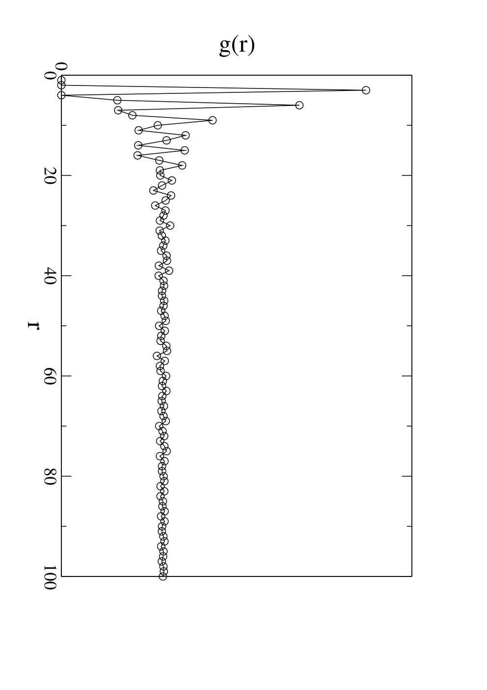
What is the origin of the “jamming”? First, “jammed” clusters do not contain flippable hexagons (by definition) but are, of course, criss-crossed by longer loops which are blocked at the temperatures considered. This implies that a typical three-coloring state must have a low-enough density of flippable hexagons. On the kagome lattice the density of flippable hexagons (averaged over the uniform ensemble) is 0.22, so that forming a large cluster of 42 sites on average is unlikely in absence of correlations. In Fig. 7, we give the correlations (radial distribution function) in the positions of the flippable hexagons of the same type.[82] We find indeed a strong attraction: the neighboring hexagons cannot be occupied by the same type of loop (it is incompatible with the constraint) but the second neighbor positions are highly favored (attraction). There is a high probability to have a flippable hexagon if the (second) neighbor is a flippable hexagon. This attraction creates aggregates and voids, opening the way to regions free of flippable hexagons. The system can therefore be viewed as a microscopic phase separation of active and inactive regions, the active regions having flippable hexagons, the inactive regions having longer loops. Recall that the degenerate model can be seen as being at the boundary of a phase transition in parameter space,[50] in particular between active and inactive phases, having respectively short and long loops.[83] This is a necessary but not a sufficient condition for the region to be “jammed” because the number of flippable hexagons is not conserved by the dynamics and they “move” on the lattice (see Fig. 1). The frozen clusters correspond to special configurations and regions inaccessible to flippable hexagons. For example, a frozen cluster of 12 sites is shown in Fig. 8: each hexagon on the border has the three possible colors A, B, C, thus making it impossible to create a flippable configuration. One can have clusters of arbitrary size (see Fig. 5) or walls that prevent flippable hexagons to diffuse in different regions of the sample.

However, a loop of length 10 (shown by a dashed line in Fig. 8) will unjam the configuration, and the cluster shown will be annihilated. The way the relaxation takes place at longer times is via the dynamics of creation and annihilation of “frozen” clusters on time-scale . For , there is a separation of time-scales between the “rapid” hexagon motion and the longer creation/annihilation of frozen clusters .
IV.4 Dynamical heterogeneities
We now consider some dynamical local quantities. Following studies of standard glasses,[4] we define a local mobility field which measures how many times the site has changed color during the time interval between 0 and . It is linear in for large so that one can define a local frequency . Frozen sites have while dynamical sites have .


The real space picture of at a given time is given in Fig. 9 from black (frozen sites) to white (fast sites): we see the variations of the local dynamics across the system and some clusters of slow frequencies, i.e. a form of dynamical heterogeneity. We plot the corresponding histogram of frequencies in Fig. 10 at various temperatures. At high temperature, the distribution is homogeneous (gaussian). At lower temperatures, the dynamics slows down, and the distribution broadens and becomes asymmetric (non zero third moment or skewness). Eventually at , a frozen fraction appears and the distribution becomes continuous between two typical peaks,
| (12) |
where is a smooth broad function. One can describe this evolution as a crossover between a homogeneous high-temperature phase with a single type of dynamical site and a low-temperature phase with many inequivalent dynamical sites. It can be described in terms of large-deviation functions and a “free-energy” can be defined.[89]
V Fragmentation of the phase-space
We show that the phase space is fragmented into a number of sectors for , separated by barriers of . For this, we directly enumerate all the states of small clusters and analyze how the system evolves in the phase-space as a function of temperature. This allows us to describe the landscape of energy barriers separating states and basins, i.e. a hierarchical organization of the states (nonfractal here).
Let be the probability of the system to be in a configuration , the total number of states which we have numerically enumerated on small clusters with periodic boundary conditions (). We have found (dashed line in Fig. 11), slightly smaller than the exact result in the thermodynamic limit .[50]
The master equation governing the dynamical evolution of ,
| (13) |
involves a matrix which contains the transition rates from a configuration to . The only allowed transitions are single flips of loops of length , where is given by Eq. 2. Here from detailed balance, we have ( for all states) and ensures the conservation of the probability, . All states satisfying
| (14) |
are stationary, such as, in particular, the equilibrium uniform distribution . may have more than one zero eigenvalue and the additional stationary states prevent the system from exploring the phase space (broken ergodicity). Examples are systems with a broken-symmetry, the phase space of which has a finite number of disconnected sectors in the thermodynamic limit. In each sector the Gibbs distribution is stationary assuring as many zero eigenvalues as the number of sectors or broken symmetries. By contrast, in a glassy-like phase, the number of eigenvalues satisfying ( is the experimental observation time) scales like : there is a finite configurational entropy . In other words, a macroscopic number of states, thus differing at the microscopic scale, never relax on the observation time-scale.
In the present model, has a finite hierarchical structure. Here it is a consequence of a microscopic model and is not assumed from the beginning as in hierarchically constrained models.[55, 84, 85] Contrary to these examples (or spin glasses[86]), however, we find only four levels of hierarchy: the phase space is split into a few “Kempe” classes,[87, 68] which are split into topological sectors and then in trapping sectors (see Fig. 11 for a graphical illustration of this hierarchy in the phase space).
V.1 Infinite barriers
The dynamics of loops of all sizes is known to be nonergodic on the kagome lattice.[51, 87] It means that moving all loops is not sufficient to go from a given state to any other state in the phase space. split in “Kempe” classes,[87, 68] the number of which is in general unknown.[87]
Since it is therefore impossible to enumerate all states by moving loops iteratively, we have allowed to introduce defects that violate the 3-colored constraint. To control the density of defects, we have introduced an energy penalty, i.e. the antiferromagnetic three-state Potts model. By cooling the system at low temperatures in a Monte Carlo simulation, one generates three-coloring ground states that are in different “Kempe” sectors (and the sectors themselves by switching on the loop dynamics). For , we find four sectors, a large one with of all states and three smaller ones, all separated by infinite barriers for the loop model.
Within each Kempe sector, the three-coloring states can be characterized by topological numbers. They are defined by counting the number of colors along nonlocal horizontal and vertical cuts.[88] There are six such numbers (), which may take any integer value from 0 to with the constraint , so four of them are independent. This gives at most sectors, but since some combinations are not allowed, the number is of order (Fig. 11). The dynamics of local loops conserves these numbers so that each Kempe sector is divided into topological sectors. Only winding loops of length or (the longest loop takes all two color sites and has length ) may change them. In fact, the averaged length of the winding loops scales like .[52, 48] The topological sectors are therefore separated by barriers growing with the system size like , defining infinite barriers in the thermodynamic limit and broken ergodicity sectors. This is analogous to the “jamming” transition induced by additional forces: the favored ordered state needs rearrangements of infinite loops in order to equilibrate.[48, 49] Here we recall that the phase space is in general broken into sectors (which we have explicitly constructed), labelled by quantities conserved by the local dynamics.[88]

V.2 Fragmentation in sectors
For , the dynamical matrix split further into new smaller sectors which we have constructed for different system sizes. We find that the phase space is split into 1.085N independent trapping sectors (Fig. 11). The spin dynamics has a fast equilibration within a sector characterized by the motion of 6-loops on time-scale and the motion between sectors occurs on time-scale, , which is frozen below by definition. Above , the system equilibrates within a topological sector.
The number of sectors defines a finite averaged configurational entropy per site , which is approximately two thirds of the full entropy . Upon reducing the temperature, the system goes from an equilibrated state with the full entropy (the number of topological sectors is sub-extensive) to a metastable state below where it looses the configurational entropy:
| (15) |
The configurational entropy reflects in phase space the entropy of the microscopic arrangements of the frozen clusters (section IV). A crude comparison consists of distributing disks on the lattice ( is the number of frozen clusters of average size , we note the density), with entropy (). This is too small though by an order of magnitude compared with .
For , one can define coarse-grained states by eliminating the fast dynamics into an entropy. While, on average, each sector contains states (thus defining the averaged entropy ), we find a broad distribution of sector sizes from (a single state) to a large sector . However, we believe that this is a finite-size effect. Indeed the probability to fall into a sector of size is found to be roughly constant at small and increases for larger sectors. In contrast, for a Monte Carlo sampling of states as done in section IV, the frozen fraction distribution is homogeneous (gaussian) for , while for , a large portion of states has no frozen fraction at all. As a consequence, the distribution of entropies is certainly more homogeneous for large system size.
In summary, we find that the phase space has hierarchical levels: it has sectors characterized by conserved quantities and separated by infinite barriers (broken ergodicity) and sectors or traps separated by finite barriers. The number of topologicals sectors is of order (nonextensive entropy), and there is no essential difference between them at the microscopic or mesoscopic scale: a local measurement cannot distinguish between two different sectors. On the other hand, the number of traps is of order (finite configurational entropy). Therefore the system looses a finite entropy at and a local disorder is self-induced: a local measurement can distinguish between two metastable states (for instance, if there is or not a frozen cluster). In this sense, can be called a glassy crossover temperature. By opposition, the jamming transition found in Refs. 48, 49 corresponds to broken ergodicity associated with a sub-extensive entropy (no self-induced disorder).
VI Discussion of experiments
We now discuss the kagome compounds that have a freezing transition. We argue that the freezing temperature is governed by the energy scale of the barriers and when possible, we identify the possible mechanisms we have discussed in section III: the barriers are either dynamically generated by the rapid spin-wave motion or generated by anisotropies, depending on specific materials. We also compare the strength of the “frozen” moment to the experiments available and the dynamics of the system. Note that the present dynamics of loops is classical (if a quantum coherence is maintained, the system was predicted to order[68]). Some quantum fluctuations are therefore neglected here, but may turn out to be important, especially for the copper oxides discussed below (), if the anisotropy is small enough.[43]
VI.1 SrCr9pGa12-9pO19 (SCGO)
In SCGO, a phase transition occurs at K, depending weakly on the Cr3+ () coverage .[13, 14, 15, 16] depends also on the experiment: K by squid, K by neutron scattering for the same compound.[20]
What could be the appropriate microscopic model? The Cr3+ ions have no orbital moment () and the spin anisotropy is expected to be small. From EPR indeed, K.[90] By constrast, the measurements of the spin susceptibility on single crystals showed a large anisotropy disappearing when increasing the temperature.[91] This was therefore attributed to the spontaneous breaking of the rotation symmetry by a nematic order (coplanarity), and not a real anisotropy of the model.[91] Similarly, the 8K barrier obtained by SR for which was originally interpreted as a large single-ion anisotropy,[92] is in fact absent if one uses a different fit of the data.[93] On the other hand, for , energy barriers of 30K were obtained.[92, 93] Since they are two orders of magnitude larger than the spin anisotropy, they are more likely to be induced by the fluctuations. With K and , we have K. On the other hand, if we use (section III) and K from the spin susceptibility, we find K. Both estimates are in fair agreement with the experimental result. The model does not predict, however, a thermodynamic transition while, experimentally, this has been a disputed point, especially regarding the sharpness of the nonlinear susceptibility .[13, 94] We also note that the “thermodynamic” anomalies we have mentionned at are not only rounded but also the entropy change is small compared with the full entropy of continuous spins. Yet this makes a definite prediction for the entropy change.
Furthermore, the frozen moment measured in neutron elastic scattering is small, of the maximum moment (depending on the Cr coverage) and most of the signal is in the inelastic channel.[17, 18, 20] In the experimental setup of Ref. 17, the inelastic channel starts above the neutron energy resolution of 0.2 meV, giving in that case a lifetime of the frozen moment longer than ps. Neutron spin-echo showed that the moment is still frozen on the nanosecond time-scale at 1.5 K.[21] However, no static moment was originally observed in SR,[95] but a weak static component may not be excluded.[93] Similarly, in Ga NMR, the wipeout of the signal shows a dynamics that has slowed down but is still persistent.[96] However, in both cases the muon or the Ga nuclei probe many sites and may see primarily the dynamical sites.
In the model developed above, the system remains dynamical below . The system has flippable hexagons on time-scale but also spin-waves on a more rapid time-scale, which we have not described. The latter should contribute to the specific heat as in normal two-dimensional antiferromagnets and give in particular a specific heat as observed experimentally.[13] This is the consequence of the two Goldstone modes associated with the selection of a common plane (nematic broken symmetry).[44]
We can make different assumptions regarding the time-scale of the activated dynamics with respect to the observation time-scale. If , the system is trapped into a typical 3-coloring on the experimental time-scale. Still the averaged moment is different from because of the rapid zero-point fluctuations of the spin-waves. One can estimate that the effect of the two Goldstone modes is to reduce the moment to .[97] For Cr3+ (), the correction is small and cannot explain the small moment measured.
Suppose now that the hexagons still have a dynamics, as indeed predicted for . We found in this case that the frozen moment is (Fig. 2). Applying the same zero-point motion reduction as above, we find which is close to the experimental frozen moment. The model therefore gives a fair account of the measured frozen moment. The small static moment is not due to strong quantum fluctuations but rather to the loop (hexagon) fluctuations.

To characterize the dynamics, we have computed the local dynamical response at different (Fig. 12). These are the Fourier transforms of the autocorrelation functions given in Fig. 2. At , and low frequencies, we have as the consequence of the universality of the height model. However, this is valid over a limited range of frequencies: in Fig. 12, the dashed lines give examples of power-laws with exponents 0.33 and 0.7, for comparison (note that all the curves are shifted horizontally by ). It is also in fairly good agreement with the observed power law behavior in neutron inelastic scattering on powders, above the transition.[17, 18, 19] When is lowered, the quasi-elastic peak corresponding to the frozen moment develops. Note that the sum-rule ensures that the apparent loss of intensity at low temperatures in Fig. 12 corresponds to a transfer into the elastic peak. Although the approach is different, we note that the exponent is not far from that obtained by dynamical mean-field theory, .[98]
In summary, the model describes a dynamical freezing crossover into a partially frozen phase and a small frozen moment in overall agreement with the experiments. The broad neutron response is interpreted as the motion of loops above . In the frozen phase, only the hexagons are predicted to move (in addition to spin waves). They could possibly be characterized by special magnetic form factors, as in ZnCr2O4.[99]
VI.2 Volborthite Cu3V2O7(OH)2.2H2O
In volborthite,[26] a freezing transition occurs at K, with a finite static moment observed by NMR[28, 29] but no long-range correlations in neutron scattering.[100] Volborthite is a slightly distorted kagome lattice and there is some current debate as to whether the main magnetic couplings are kagome like or more one-dimensional.[101] We will assume below that it can be viewed as a kagome antiferromagnet and that the distortion is a small effect.
Below the transition, NMR revealed that the phase is heterogeneous with a time-dependent lineshape, leading to distinguish between “fast” and “slow” (static) sites, either at small fields[28] or in a dinstinct phase,[29] at larger fields.[31]
These results resemble the dynamical heterogeneities found in the model below . We can make a more detailed comparison by computing the distribution of fields. NMR was performed on vanadium nuclei which seat at the centers of the hexagons.[28, 29] The nuclei see effective fields averaged over the six sites of a hexagon (assuming for simplicity the same hyperfine coupling ),
| (16) |
which depend on the hexagon (inhomogeneous broadening). An average over the NMR time scale is taken. In principle is much larger s than the microscopic time-scales ps, and can be taken to . In systems with slow dynamics, NMR probes local trajectories averaged over . The lineshape depends on , thus providing information on the presence of dynamical heterogeneities. The lineshape is related to the distribution function of field strengths , which we have calculated in the present case.


We expect different regimes, according to whether the NMR time-scale is shorter or longer than the characteristic time-scales of the dynamics, and . Note that since these describe activated processes, they may become much longer than the ps microscopic time at low temperatures.
- •
. The system equilibrates on NMR time-scales, e.g. at high-. Every site has dynamics and summing random vectors (at 120o though) gives a gaussian distribution of fields (dashed line in Fig. 13). For , summing local fields corresponds to a random walk and the typical strength since we have no external field.
- •
. The system is completely frozen in a typical three-coloring state. Each nucleus sees a well defined static field. For a 3-coloring, there are only three possible field strengths at the center of the hexagon, (see the configurations shown in Fig. 13, top). Averaging over the uniform ensemble, we find three peaks with weight 18, 60, 22 (22 is the fraction of flippable hexagons). For comparison, the antiferromagnetic state would have a single peak at with 100 of the hexagons and the state a single peak at .
- •
. The system is out-of-equilibrium below , by definition. The dynamical sites provide a time-dependent averaged field (broad part of the lineshape in Fig. 13). The frozen sites inside the clusters provide a static field: we find two peaks at and and no peak at which corresponds to the flippable hexagons. Although the local field does not change when they flip, the probability that they remain in a flippable configuration is small. Instead they move on the lattice and there are very few isolated flippable hexagons inside frozen clusters. We further note that the static fields inside the frozen clusters show a ratio much larger than that of a typical state (Fig. 13). This means that the frozen clusters resemble locally to the state, the state with long linear winding loops, precisely those which do not flip.
Experimentally, in volborthite, the NMR lineshape consists of two dynamically heterogeneous contributions at .[31] A slow “rectangular” shape was assigned to a static field (the “rectangular” shape arising from the powder convolution) and a fast gaussian contribution to dynamical sites.[31] Similar results were obtained at low fields on lower-quality samples.[28]
The low-field results can be compared with Fig. 13 (up to a powder convolution). For we find two contributions: (i) a static contribution coming from the frozen clusters and represented by two peaks at and , the latter giving rise to a rectangular shape in a powder sample. (ii) a dynamical part resulting from the dynamical regions and giving rise to a broad response. Here we do not have a single dynamical site but this is not necessarily incompatible with the experiments because of the difficulty of resolving different sites. We also note that the respective contribution of both is smaller than the 50-50 observed experimentally,[31] but this depends on the time-scale.
Assuming that the system had a character and that the static field was therefore due to the types of hexagons, a small frozen moment of 0.41 per site was extracted.[28] In the present model, a peak at is not compatible with the existence of dynamical sites. Instead we assign the experimental peak to the frozen field. In this case, instead of ,[28] the static moment is (as also proposed in Ref. 47 for different reasons), which is more compatible with conventional on-site zero-point fluctuations, . Moreover, if we now calculate the total frozen moment averaged over all sites as measured by neutrons (while NMR sees the full local frozen moment), we would predict .
We conclude that the present study gives a model for the phase transition and the heterogeneous state observed in volborthite. Similarly to SCGO, it gives an interpretation for the small moment observed for : the fluctuations of small loops reduce the averaged moment. The model suggests a more precise picture of frozen clusters with an emergent length scale, that can be further tested experimentally.
VI.3 Vesignieite Cu3BaV2O8(OH)2
For vesignieite,[27] K, and the ground state is also heterogeneous: approximately 50 of the sites (muon sites and nucleus sites) experience a static field.[32, 30] The loss of 50 of the total intensity in NMR is due to the nuclei which have a time-scale that cannot be detected, and therefore reflects some dynamical heterogeneities in the local environment. It would be inaccurate to consider that the 50 of the observed intensity is due to the spins in the frozen clusters and the missing 50 due to the fast moving spins. It may well be that some dynamical sites of Fig. 13 are detected (this is in fact what we assumed for the volborthite where 100 of the nuclei were detected). The fact that the fraction does not match the number of frozen sites of 12 is not therefore a serious drawback. Alternatively the fraction of frozen sites certainly depends on the interactions. For Dzyaloshinskii-Moriya interactions which are present and may be rather strong,[32] the frozen fraction will certainly increase because it favors the state with long loops.
VI.4 Hydronium jarosite, (H3O)Fe3(SO4)2(OH)6
A freezing transition occurs at 15K.[22] By varying sample preparations, 12K-18K and it appears to be weakly sensitive to the Fe coverage in the range 92-100.[23] Neutron elastic scattering has found short-range correlations of the type, but no long-range order.[102, 103, 40] The Heisenberg coupling is K (),[40] so that which in terms of a classical Heisenberg model means that the system should be in the collective paramagnetic regime.[57] One clearly needs some additional ingredients to explain the freezing transition.
Spin anisotropy is known to be present in a similar jarosite compound, KFe3(SO4)2(OH)6, both single-ion easy-plane anisotropy K and a Dzyaloshinskii-Moriya interaction K explaining the excitation spectrum.[104, 105] X-ray dichroism of the Fe3+ ion also found a single-ion anisotropy in good agreement with the above figure.[106] In addition, in ordered jarosite compounds, a second transition corresponding to the in-plane locking of the spins occurs at K.[107] With these large values in mind, we assume that the energy barriers of the model originate in the anisotropy. In this case, we can predict and compare with that obtained from ac-susceptibility measurements.[24] Since, in the model, we have for s (Hz), and K, we find K. Similarly, for ms (80Hz), we find K. These estimates are a little smaller than the experimental figures and depends more strongly on the measurement frequency (the same distinction occurs in structural glasses between “fragile” and “strong” glasses).[24] Moreover, by varying synthesis conditions, was found to be correlated with the distortion of the FeO6 octahedra: the stronger the distortion the larger the .[108] Since the octahedron distortion implies a linear change in the crystal field splitting, hence in the single-ion anisotropy , we expect indeed linear changes in , as observed experimentally.[108]
For , an estimate of the frozen moment has been obtained by SR and amounts to 3.4 compared with 5.92 of the Fe3+ ion,[109] so that . It is not far from the present estimate . However, it is surprising that similar values were obtained in ordered jarosites.[109]
For , neutron inelastic scattering has been performed and showed that the local response, .[40] At very low frequency, we have found but at larger frequencies it could be fitted by a larger exponent (the second dashed line in Fig. 12 corresponds to ). The agreement is therefore qualitative with a broad increasing response by lowering the frequency (to be contrasted with the flat response of a conventional two-dimensional antiferromagnet) but a single exponent is not found.
To conclude, the present study suggests that in (H3O)Fe3(SO4)2(OH)6 is related to a dynamical freezing into a heterogeneous state. The relevant energy scale here, contrary to SCGO, is the anisotropy, as experimentally claimed.[108] Below , we expect a small frozen moment on average and a persistent dynamics of the hexagons, which distinguishes the present transition from a complete dynamical arrest. More studies of the low-temperature phase would be interesting.
VI.5 Other kagome compounds, competitions
It is well known that not all kagome compounds have a freezing transition and we briefly discuss some other compounds. Some have magnetic long-range order, which is often accounted by additional spin interactions. Others, such as the herbertsmithite compounds ZnCu3(OH)6Cl2[111] and MgCu3(OH)6Cl2,[112] have no freezing transition (unless an external field is applied[113]) and no long-range order.[110] The neutron inelastic response has no clear energy scale in ZnCu3(OH)6Cl2[38] and is fitted by a broad power law at low enough energy,[37, 39] with some similarity with that of SCGO and the hydronium jarosite above . In the present model, one would interpret this result as being in the phase above , and the neutron inelastic response agrees qualitatively with Fig. 12. However, the reason why would be smaller than the lowest temperatures reached experimentally, say 50 mK, is not clear. We have argued that is controlled by the anisotropy (dynamically-generated or not), and the anisotropy is present in ZnCu3(OH)6Cl2.[114, 115] Two important effects are missing: it is known that antisite disorder is present,[116] and that compounds have strong quantum effects with currently debated quantum spin liquid phases if the anisotropy is sufficiently weak (such a coupling may discriminate between different phases in compounds[43]). It is therefore clear that competitions are important to account for all these phases.
VII Conclusion
We have described a simple spin model which has a dynamical glassy-like freezing at a crossover temperature , in absence of any quenched disorder.
The system evolves from a dynamically homogeneous phase with a single time-scale () to a dynamically heterogeneous phase with two time-scales (). The first time-scale corresponds to the “rapid” degrees of freedom, the shortest loops. The second time-scale is associated with the rearrangement of the “frozen” clusters. The frozen clusters have a microscopic length-scale (they typically contain a few tens of sites) but their rearrangement time is not controlled by the their size but by the size of the second shortest loops, . When becomes longer than the experimental time-scale for , the system is out-of-equilibrium and glassy-like. The clusters contain spins that are frozen on the experimental time-scale and realize a microscopic-scale disorder. In this case, the system has a finite (small) averaged frozen moment but no true long-range order. We have explained that the frozen moment is due, partly to the frozen clusters themselves and, partly to dynamical regions where the spins are strongly constrained by the frozen regions.
The phase space of the system appears to be organized in a partially hierarchical manner with conserved quantities defining basins separated by infinite barriers (broken ergodicity). Each basin was shown to further split into sectors separated by finite barriers which trap the system in a metastable state below . This macroscopic fragmentation of the phase space corresponds to the local disorder induced by the “frozen” clusters. At , the system has therefore some “thermodynamic” anomalies characterized by the loss of the configurational entropy which we have calculated by finite-size scaling, per site.
The system undergoes a glassy-like transition at because the residual “rapid” degrees of freedom (the shortest loops) only partially reorganize the system. In a typical state, the density of the shortest loops is not very small, but, by effectively attracting each other, they form aggregates and voids (micro phase separation), the latter regions being, hence, frozen. Some details, as to what their density is, or how they precisely interact, certainly depend on the system and the model, but the mechanism we have presented here is rather clear: the strong local correlations generate slow extended degrees of freedom which, since they are correlated and attract each other, “phase-separate” in dense active regions and void inactive regions.
Several aspects of the degenerate model are simply assumed. We have assumed the absence of long-range order by considering degenerate states (Eq. 1), and an activated relaxation time (Eq. 2); hence, not surprisingly, the dynamics is slow. We have discussed in section III why both assumptions may be approximately realized in microscopic models with continuous degrees of freedom. We argued that the origin of the energy barriers is the partial order-by-disorder, i.e. the barriers are dynamically generated by the rapid spin-waves, or by an explicit anisotropy arising from the spin-orbit coupling. The degeneracy (Eq. 1) is in general not exact and lifting it favors a “crystal” state in the energy landscape without modifying -if it remains sufficiently small- the dynamical aspects we have described.
We have compared the results with the experiments on the kagome compounds. The present study gives a model for the spin freezing observed at and provides an interpretation for the nature of the low-temperature phase. The picture of the “frozen” phase that emerges is that of an heterogeneous state with dynamical and frozen regions. The weak measured frozen moment is interpreted as the consequence of the remaining dynamics of the shortest loops and its strength is close to what is measured in the experiments. While in magnets in general, the on-site moment is reduced by the small oscillations around the ordered state (spin-waves), here the main effect is argued to be the large-amplitude motion of the shortest loops. The short loop fluctuations do not fully destroy the moment for but their presence is in agreement with the persistent fluctuations observed by different experimental techniques (neutrons, SR, NMR). In particular, the observation in NMR of nuclei with different time-scales is consistent with the heterogeneous picture of the dynamics proposed here. In conventional magnets, the thermal excitations of the spin-waves destroy the on-site magnetization. Here, one needs longer loops, that are thermally excited only for . These fluctuations give a spectral response that obeys a power-law in the small energy limit, very different from that of conventional magnets (flat response in two dimensions). A broad power-law response is indeed observed experimentally in neutron inelastic scattering. Although the exponent seems to be underestimated, the experiments may not have had access to the low-energy limit or the exponent may be inacurately predicted because of the interaction between the spin-waves and the discrete modes. In the paramagnetic phase, the model has algebraic spatial correlations at equilibrium (), a feature that is not observed in elastic neutron scattering. We believe that this is not redhibitory, for the spin freezing we have described is not related to the long-distance behavior. In two spatial dimensions, the correlation length is always finite at finite temperatures.[117] Furthermore, the chemical disorder is present to an amount which is difficult to quantify and which has been completely neglected here.
The energy scale that governs the freezing temperature is argued to be in the small anisotropy limit (dynamically generated barriers), and it crosses over to in the strong anisotropy limit, typically if . This led us to a tentative classification, where SCGO is in the small anisotropy limit and (H3O)Fe3(SO4)2(OH)6 in the strong anisotropy limit. This is clearly a different interpretation from that of chemical disorder, where is governed by the amount of disorder.[3]
In order to disentangle intrinsic effects from the effects of chemical disorder, one can test the present theory, in particular by characterizing experimentally the active magnetic degrees of freedom, for instance by neutron form factors,[99] or by inferring the nanoscopic size of the frozen clusters.
Acknowledgements.
O. C. would like to thank J.-C. Anglès d’Auriac, F. Bert, L. Cugliandolo, B. Douçot, B. Fåk, D. Levis, C. Lhuillier, P. Mendels, H. Mutka, G. Oshanin, and J. Villain for discussions and especially A. Ralko for continuing collaboration. B. C. would like to thank M. Taillefumier, J. Robert, C. Henley and R. Moessner for discussions and collaboration on related projects. O. C. was partly supported by the ANR-09-JCJC-0093-01 grant.References
- [1] J. Villain, Z. Physik B 33, 31 (1979).
- [2] L. Bellier-Castella, M. J. P. Gingras, P. C. W. Holdsworth, and R. Moessner, Can. J. Phys. 79, 1365 (2001).
- [3] T. E. Saunders and J. T. Chalker, Phys. Rev. Lett. 98, 157201 (2007).
- [4] Dynamical heterogeneities in glasses, colloids and granular materials, Eds. L. Berthier, G. Biroli, J.-P. Bouchaud, L. Cipelletti, W. van Saarloos (Oxford University Press, Oxford, 2011).
- [5] D. Kivelson, S. A. Kivelson, X. Zhao, Z. Nussinov, G. Tarjus, Physica A, 219, 27 (1995).
- [6] J. Villain and S. Aubry, phys. stat. sol. 33, 337 (1969).
- [7] C. Donati, J. F. Douglas, W. Kob, S. J. Plimpton, P. H. Poole, and S. C. Glotzer, Phys. Rev. Lett. 80, 2338 (1998).
- [8] J. S. Langer, Phys. Rev. E 73, 041504 (2006).
- [9] J. S. Gardner, B. D. Gaulin, S.-H. Lee, C. Broholm, N. P. Raju, and J. E. Greedan, Phys. Rev. Lett. 83, 211 (1999).
- [10] J. Snyder, J. S. Slusky, R. J. Cava, and P. Schiffer, Nature 413, 48 (2001).
- [11] For a review, see the chapters by M. J. P. Gingras, R. Moessner and K. S. Raman, in Highly Frustrated Magnetism, edited by C. Lacroix, P. Mendels, F. Mila (Springer Verlag, Berlin, 2010).
- [12] X. Obradors, A. Labarta, A. Isalgué, J. Tejada, J. Rodriguez, M. Pernet, Solid State comm. 65, 189 (1988).
- [13] A. P. Ramirez, G. P. Espinosa, and A. S. Cooper, Phys. Rev. Lett. 64, 2070 (1990).
- [14] A. P. Ramirez, G. P. Espinosa, and A. S. Cooper, Phys. Rev. B 45, 2505 (1992).
- [15] B. Martínez, F. Sandiumenge, A. Rouco, A. Labarta, J. Rodríguez-Carvajal, M. Tovar, M. T. Causa, S. Galí, and X. Obradors, Phys. Rev. B 46, 10786 (1992).
- [16] A. P. Ramirez, Annu. Rev. Mater. Sci. 24, 453 (1994).
- [17] C. Broholm, G. Aeppli, G. P. Espinosa, and A. S. Cooper, Phys. Rev. Lett. 65, 3173 (1990).
- [18] S.-H. Lee, C. Broholm, G. Aeppli, A. P. Ramirez, T. .G. Perring, C. .J. Carlile, M. Adams, T. J. L. Jones, and B. Hessen, EPL 35 (2), 127 (1996).
- [19] C. Mondelli, H. Mutka, C. Payen, B. Frick, K. H. Andersen, Physica B, 284, 1371 (2000).
- [20] C. Mondelli, H. Mutka, and C. Payen, Can. J. Phys. 79, 1401 (2001).
- [21] H. Mutka, G. Ehlers, C. Payen, D. Bono, J. R. Stewart, P. Fouquet, P. Mendels, J. Y. Mevellec, N. Blanchard, and G. Collin, Phys. Rev. Lett. 97, 047203 (2006).
- [22] A. S. Wills, A. Harrison, C. Ritter, and R. I. Smith, Phys. Rev. B 61, 6156 (2000).
- [23] A. S. Wills and W. G. Bisson, J. Phys.: Condens. Matter 23, 164206 (2011).
- [24] A. S. Wills, V. Dupuis, E. Vincent, J. Hammann, and R. Calemczuk, Phys. Rev. B 62, 9264(R) (2000).
- [25] F. Ladieu, F. Bert, V. Dupuis, E. Vincent, and J. Hammann, J. Phys.: Condens. Matter 16, S735 (2004).
- [26] Z. Hiroi, M. Hanawa, N. Kobayashi, M. Nohara, H. Takagi, Y. Kato and M. Takigawa, J. Phys. Soc. Jpn. 70, 3377 (2001).
- [27] Y. Okamoto, H. Yoshida, Z. Hiroi, J. Phys. Soc. Jpn. 78, 033701 (2009).
- [28] F. Bert, D. Bono, P. Mendels, F. Ladieu, F. Duc, J.-C. Trombe, and P. Millet, Phys. Rev. Lett. 95, 087203 (2005).
- [29] M. Yoshida, M. Takigawa, H. Yoshida, Y. Okamoto, and Z. Hiroi, Phys. Rev. Lett. 103, 077207 (2009).
- [30] R. H. Colman, F. Bert, D. Boldrin, A. D. Hillier, P. Manuel, P. Mendels, and A. S. Wills, Phys. Rev. B 83, 180416(R) (2011).
- [31] M. Yoshida, M. Takigawa, H. Yoshida, Y. Okamoto, and Z. Hiroi, Phys. Rev. B 84, 020410(R)(2011).
- [32] J. A. Quilliam, F. Bert, R. H. Colman, D. Boldrin, A. S. Wills, and P. Mendels, Phys. Rev. B 84, 180401(R) (2011).
- [33] Note that “dynamical heterogeneity” is used in a sense slightly different from that used in structural glasses,[4] since dynamical correlations are not probed in NMR. What it literally means is that there are sites with different dynamics.
- [34] P. Schiffer, A. P. Ramirez, D. A. Huse, P. L. Gammel, U. Yaron, D. J. Bishop, and A. J. Valentino, Phys. Rev. Lett. 74, 2379 (1995).
- [35] E. Lhotel, V. Simonet, J. Ortloff, B. Canals, C. Paulsen, E. Suard, T. Hansen, D. J. Price, P. T. Wood, A. K. Powell, and R. Ballou, Phys. Rev. Lett. 107, 257205 (2011).
- [36] P. Mendels, F. Bert, M. A. de Vries, A. Olariu, A. Harrison, F. Duc, J. C. Trombe, J. S. Lord, A. Amato, and C. Baines, Phys. Rev. Lett. 98, 077204 (2007).
- [37] J. S. Helton, K. Matan, M. P. Shores, E. A. Nytko, B. M. Bartlett, Y. Yoshida, Y. Takano, A. Suslov, Y. Qiu, J.-H. Chung, D. G. Nocera, and Y. S. Lee, Phys. Rev. Lett. 98, 107204 (2007).
- [38] M. A. de Vries, J. R. Stewart, P. P. Deen, J. O. Piatek, G. J. Nilsen, H. M. Rønnow, and A. Harrison, Phys. Rev. Lett. 103, 237201 (2009).
- [39] J. S. Helton, K. Matan, M. P. Shores, E. A. Nytko, B. M. Bartlett, Y. Qiu, D. G. Nocera, and Y. S. Lee, Phys. Rev. Lett., 104, 147201 (2010).
- [40] B. Fåk, F. C. Coomer, A. Harrison, D. Visser, and M. E. Zhitomirsky, EPL 81, 17006 (2008).
- [41] A. B. Harris, C. Kallin, and A. J. Berlinsky, Phys. Rev. B 45, 2899 (1992).
- [42] M. Elhajal, B. Canals, and C. Lacroix, Phys. Rev. B 66, 014422 (2002).
- [43] O. Cépas, C. M. Fong, P.W. Leung, and C. Lhuillier, Phys. Rev. B 78, 140405(R) (2008).
- [44] I. Ritchey, P. Chandra, and P. Coleman, Phys. Rev. B 47, 15342 (1993); P. Chandra, P. Coleman, I. Ritchey, J. Phys. I France 3, 591 (1993).
- [45] G. Aeppli and P. Chandra, Science 275, 177 (1997).
- [46] M. Ferrero, F. Becca, and F. Mila, Phys. Rev. B 68, 214431 (2003).
- [47] F. Wang, A. Vishwanath, and Y. B. Kim, Phys. Rev. B 76, 094421 (2007).
- [48] B. Chakraborty, D. Das, and J. Kondev, Eur. Phys. J. E 9, 227 (2002).
- [49] C. Castelnovo, P. Pujol, and C. Chamon, Phys. Rev. B 69, 104529 (2004).
- [50] R. J. Baxter, J. Math. Phys. 11, 784 (1970).
- [51] D. A. Huse, and A. D. Rutenberg, Phys. Rev. B 45, 7536 (1992).
- [52] J. Kondev and C. L. Henley, Phys. Rev. Lett. 74, 4580 (1995).
- [53] C. L. Henley, Ann. Rev. Cond. Matt. 1, 179 (2010).
- [54] C. L. Henley, J. Stat. Phys. 89, 483 (1997).
- [55] R. G. Palmer, D. L. Stein, E. Abrahams, and P. W. Anderson, Phys. Rev. Lett. 53, 958 (1984).
- [56] G. H. Fredrickson and H. C. Andersen, Phys. Rev. Lett. 53, 1244 (1984).
- [57] J. T. Chalker, P. C. W. Holdsworth, and E. .F. Shender, Phys. Rev. Lett. 68, 855 (1992).
- [58] J. N. Reimers and A. J. Berlinsky, Phys. Rev. B 48, 9539 (1993).
- [59] M. E. Zhitomirsky, Phys. Rev. B 78, 094423 (2008).
- [60] A. V. Chubukov, Phys. Rev. Lett. 69, 832 (1992).
- [61] C. L. Henley and E. P. Chan, J. Magn. Magn. Mat. 140-144, 1693 (1995).
- [62] C. L. Henley, Phys. Rev. B 80, 180401 (2009).
- [63] S. Sachdev, Phys. Rev. B 45, 12377 (1992).
- [64] L. Messio, B. Bernu, and C. Lhuillier, arXiv:1110.5440.
- [65] J. Villain, R. Bidaux, J. P. Carton and R. Conte, J. Phys. (Paris) 41, 1263 (1980).
- [66] C. L. Henley, Phys. Rev. Lett. 62, 2056 (1989).
- [67] J. von Delft and C. L. Henley, Phys. Rev. B 48, 965 (1993).
- [68] O. Cépas and A. Ralko, Phys. Rev. B 84, 020413 (2011).
- [69] U. Weiss, Quantum dissipative systems, World Scientific Publishing, Singapore 2008.
- [70] Such axis result from crystal fields and must be compatible with the local symmetry (e.g. the axis pointing towards the center of the hexagon is in general different from the other two, ).
- [71] J. V. José, L. P. Kadanoff, S. Kirkpatrick, and D. R. Nelson, Phys. Rev. B 16, 1217 (1977).
- [72] S. Tanaka and S. Miyashita, J. Phys. Soc. Jpn. 76, 103001 (2007).
- [73] C. Castelnovo, R. Moessner, S. L. Sondhi, Phys. Rev. Lett. 104, 107201 (2010).
- [74] D. Levis, L. F. Cugliandolo, EPL 97, (3), 30002 (2012).
- [75] A. Rahman and F. H. Stillinger, J. Chem. Phys. 57, 4009 (1972).
- [76] R. G. Melko, B. C. den Hertog, M. J. P. Gingras, Phys. Rev. Lett. 87, 067203 (2001); R. G. Melko, M. Enjalran, B. C. den Hertog, M. J. P. Gingras, J. Phys.: Condens. Matter 16, R1277 (2004).
- [77] L. D. C. Jaubert, M. Haque, and R. Moessner, Phys. Rev. Lett. 107, 177202 (2011).
- [78] M. Grousson, G. Tarjus, and P. Viot, Phys. Rev. E 65, 065103(R) (2002).
- [79] N. Read, proceedings of the kagome workshop, Jan. 1992 (unpublished). We thank C. Henley for communicating this to us.
- [80] J. Kondev and C. L. Henley, Nucl. Phys. B 464, 540 (1996).
- [81] The equivalent quantum model at can be written down in 2+1 dimensions; the locking potential (Coulomb charges) is relevant in the renormalisation group sense and the system was conjectured to order in the ground state,[79] which was recently confirmed numerically by using a microscopic model.[68] Dimensional reduction leads to Eq. 7 above a deconfinement crossover temperature.[68]
- [82] We would like to thank G. Oshanin for suggesting this.
- [83] In terms of spin structures indeed (see Ref. 41 for the definitions of the structures) the state is the one which maximizes the number of flippable hexagons (staggered chiralities), while the state (all triangles in the same ABC state with uniform chiralities) has infinite loops scaling with the linear size of the system. The first (resp. second) is favored by a ferromagnetic (resp. antiferromagnetic) second-neighbor interaction (here ).
- [84] G. Paladin, M. Mézard, and C. de Dominicis, J. Physique Lett. 46 L-985 (1984); A. T. Ogielski and D. L. Stein, Phys. Rev. Lett. 55, 1634 (1985).
- [85] R. Mélin, J.-C. Anglès d’Auriac, P. Chandra, and B. Douçot, J. Phys. A, 29, 5773 (1996).
- [86] M. Mézard, G. Parisi, N. Sourlas, G. Toulouse, and M. Virasoro, Phys. Rev. Lett. 52, 1156 (1984).
- [87] B. Mohar and J. Salas, J. Stat. Mech. P05016 (2010).
- [88] C. Castelnovo, C. Chamon, C. Mudry, and P. Pujol, Phys. Rev. B 72, 104405 (2005).
- [89] J. P. Garrahan, R. L. Jack, V. Lecomte, E. Pitard, K. van Duijvendijk, and F. van Wijland, Phys. Rev. Lett. 98, 195702 (2007).
- [90] H. Ohta, M. Sumikawa, M. Motokawa, H. Kikuchi and H. Nagasawa, J. Phys. Soc. Jpn. 65, 848 (1996).
- [91] P. Schiffer, A. P. Ramirez, K. N. Franklin, and S-W. Cheong, Phys. Rev. Lett. 77, 2085 (1996).
- [92] A. Keren, Y. J. Uemura, G. Luke, P. Mendels, M. Mekata, and T. Asano, Phys. Rev. Lett. 84, 3450 (2000).
- [93] D. Bono, P. Mendels, G. Collin, N. Blanchard, F. Bert, A. Amato, C. Baines, and A. D. Hillier, Phys. Rev. Lett. 93, 187201 (2004).
- [94] B. Martínez, A. Labarta, R. Rodrìguez-Solá, and X. Obradors, Phys. Rev. B 50, 15779 (1994).
- [95] Y. J. Uemura, A. Keren, K. Kojima, L. P. Le, G. M. Luke, W. D. Wu, Y. Ajiro, T. Asano, Y. Kuriyama, M. Mekata, H. Kikuchi, and K. Kakurai, Phys. Rev. Lett. 73, 3306 (1994).
- [96] L. Limot, P. Mendels, G. Collin, C. Mondelli, B. Ouladdiaf, H. Mutka, N. Blanchard, and M. Mekata, Phys. Rev. B 65, 144447 (2002).
- [97] O. Cépas and A. Ralko, unpublished.
- [98] A. Georges, R. Siddharthan, and S. Florens, Phys. Rev. Lett. 87, 277203 (2001).
- [99] S.-H. Lee, C. Broholm, W. Ratcliff, G. Gasparovic, Q. Huang, T.H. Kim, S.-W. Cheong, Nature 418, 856 (2002).
- [100] G. J. Nilsen, F. C. Coomer, M. A. de Vries, J. R. Stewart, P. P. Deen, A. Harrison, and H. M. Rønnow, Phys. Rev. B 84, 172401 (2011).
- [101] O. Janson, J. Richter, P. Sindzingre, and H. Rosner, Phys. Rev. B 82, 104434 (2010).
- [102] A. S. Wills, A. Harrison, S. A. M. Mentink, T. E. Mason and Z. Tun, Europhys. Lett. 42, 325 (1998).
- [103] A. S. Wills, G. S. Oakley, D. Visser, J. Frunzke, A. Harrison, and K. H. Andersen, Phys. Rev. B 64, 094436 (2001).
- [104] K. Matan, D. Grohol, D. G. Nocera, T. Yildirim, A. B. Harris, S. H. Lee, S. E. Nagler, and Y. S. Lee, Phys. Rev. Lett. 96, 247201 (2006).
- [105] T. Yildirim and A. B. Harris, Phys. Rev. B 73, 214446 (2006).
- [106] M. A. de Vries, T. K. Johal, A. Mirone, J. S. Claydon, G. J. Nilsen, H. M. Rønnow, G. van der Laan, and A. Harrison, Phys. Rev. B 79, 045102 (2009) .
- [107] J. Frunzke, T. Hansen, A. Harrison, J. S. Lord, G. S. Oakley, D. Visser and A. S. Wills, J. Mater. Chem., 11, 179 (2001).
- [108] W. G. Bisson and A. S. Wills, J. Phys.: Condens. Matter 20, 452204 (2008).
- [109] A. Harrison, K. M. Kojima, A. S. Wills, Y. Fudamato, M. I. Larkin, G. M. Luke, B. Nachumi, Y. J. Uemura, D. Visser, J.S. Lord, Physica B: Condensed Matter, 289, 217 (2000).
- [110] For a review, see P. Mendels and F. Bert, J. Phys. Soc. Jpn. 79, 011001 (2010).
- [111] M. P. Shores, E. A. Nytko, B. M. Bartlett, and D. G. Nocera, J. Am. Chem. Soc. 127, 13462 (2005).
- [112] E. Kermarrec, P. Mendels, F. Bert, R. H. Colman, A. S. Wills, P. Strobel, P. Bonville, A. Hillier, and A. Amato, Phys. Rev. B 84, 100401 (2011).
- [113] M. Jeong, F. Bert, P. Mendels, F. Duc, J. C. Trombe, M. A. de Vries, and A. Harrison, Phys. Rev. Lett. 107, 237201 (2011).
- [114] A. Zorko, S. Nellutla, J. van Tol, L. C. Brunel, F. Bert, F. Duc, J. C. Trombe, M. A. de Vries, A. Harrison, and P. Mendels, Phys. Rev. Lett. 101, 026405 (2008).
- [115] S. El Shawish, O. Cépas, and S. Miyashita, Phys. Rev. B 81, 224421 (2010).
- [116] A. Olariu, P. Mendels, F. Bert, F. Duc, J. C. Trombe, M. A. de Vries, and A. Harrison, Phys. Rev. Lett. 100, 087202 (2008).
- [117] For continuous spins, following [S. Chakravarty, B. I. Halperin, and D. R. Nelson, Phys. Rev. B 39, 2344 (1989)] in the small anisotropy limit, at , is rather large. Similarly, defects violating the local constraint introduce a finite correlation length.