Periodic Cosmological Evolutions of Equation of State for Dark Energy
Abstract
We demonstrate two periodic or quasi-periodic generalizations of the Chaplygin gas (CG) type models to explain the origins of dark energy as well as dark matter by using the Weierstrass , and functions with two periods being infinite. If the universe can evolve periodically, a non-singular universe can be realized. Furthermore, we examine the cosmological evolution and nature of the equation of state (EoS) of dark energy in the Friedmann-Lemaître-Robertson-Walker cosmology. It is explicitly illustrated that there exist three type models in which the universe always stays in the non-phantom (quintessence) phase, whereas it always evolves in the phantom phase, or the crossing of the phantom divide can be realized. The scalar fields and the corresponding potentials are also analyzed for different types of models.
pacs
95.36.+x, 98.80.-kI Introduction
Inflation in the early universe has been confirmed by the recent observations of cosmic microwave background (CMB) radiation [1, 2, 3, 4]. In addition, the accelerated expansion of the current universe has also been suggested by recent observations, e.g., Type Ia Supernovae [5, 6], CMB radiation [1, 2, 3, 4], the large scale structure LSS [7, 8], baryon acoustic oscillations (BAO) [9], and weak lensing [10]. To explain such a cosmic acceleration, one provides the existence of so-called dark energy in the framework of general relativity (for reviews, see, e.g., [11, 12, 13, 14, 15, 16, 17, 18]), or one supposes that gravity is modified on the large scale (for reviews, see, e.g., [19, 20, 21, 22, 23, 24, 25, 26]).
In the expansion history of the universe, there exist two singularities. One is a Big Bang singularity. The other is the finite-time future singularities [27, 28, 29, 30, 31, 32, 33, 34, 35, 36, 37, 38, 39, 40, 41, 42, 43, 44, 45, 46, 47, 48, 49, 50, 51, 52, 53, 54, 55, 56, 57, 58, 59, 60, 61, 62, 63, 64, 65, 66, 67, 68, 69, 70, 71, 72, 73, 74], which occurs at the last stage of the universe filled with dark energy, or a Big Crunch singularity. To avoid these singularities, various cosmological scenarios have been proposed, e.g., the cyclic universe [75, 76, 77, 78, 79, 80, 81, 82, 83, 84, 85] (for a reference in a different context, see [86]), the ekpyrotic scenario [87, 88, 89, 77], and the bouncing universe [90, 91, 92, 93, 94, 95, 96, 97, 98, 99, 100, 101]. Furthermore, related to the cyclic universe, the (trefoil and figure-eight) knot universe has been investigated in Ref. [102, 103, 104, 105]. In addition, motivated by the studies on the role of applying the Weierstrass , and -functions and the Jacobian elliptic functions to astrophysics and cosmology [106, 107, 108, 109, 110], the equation of state (EoS) for the cyclic universes in the homogeneous and isotropic Friedmann-Lemaître-Robertson-Walker (FLRW) spacetime has been reconstructed by using the Weierstrass and Jacobian elliptic functions in Ref. [111].
In this paper, based on the reconstruction method in Refs. [19, 20, 71, 55, 61], with the Weierstrass -function, we examine the cosmological evolution of the EoS for dark energy in FLRW cosmology. In particular, it is shown that two periodic generalized Chaplygin gas (GCG) type models for dark energy can be reconstructed. To account for the origins of dark energy as well as dark matter with a fluid, the original CG [112], GCG [113] and the modified CG (MGC) [114, 116] have been explored. We mention that the reconstruction of periodic cosmologies have widely been studied. Especially, the reconstruction of periodic EoS has been investigated, e.g., in Ref. [115]. In this reference, with an inhomogeneous EoS for dark energy fluid, it has been demonstrated that an oscillating universe can occur. Also, the Hubble parameter with a periodic behavior can realize both inflation in the early universe and the late-time cosmic acceleration under the same mechanism in a unified manner. In addition, it has been verified that a coupling between dark energy fluid, which has a homogeneous and constant EoS, and matter, can present a periodic behavior of the universe. Furthermore, as several theoretical issues in the universe with its oscillatory behavior, the phantom phase and finite-time future singularities have been investigated. A scalar-tensor description of the oscillating universe has also been explored. As stated, there exist various theoretical subjects in the periodic cosmological evolution of the universe. The essential property of the Weierstrass functions is to have two periods and . Hence, the periodical and quasiperiodical models which we show in Sec. 3 are periodical or quasiperiodical in terms of the energy density . In addition, these models with the periods and being infinite are reduced to the Chaplygin gas models (as is seen from the formulae in Eq. (6)). Thus, the reconstruction procedure of these models corresponds to two periodic or quasi periodical generalizations of the CG models. This justifies the use of the Weierstrass functions in cosmological models. Furthermore, the models given in Sec. 4 are periodic on the cosmic time (which is a dimensionless quantity in our analysis), although the models in Sec. 3 are periodic/quasiperiodic on . The periodicity of the cosmological evolution comes from the periodic nature of the Weierstrass functions. Also, the periodic/quasiperiodic models in Sec. 3 are singular at , whereas those in Sec. 4 are singular at . If the periodic evolution of the universe can be realized, various scenarios to avoid cosmological singularities can be constructed. This is the important cosmological motivation to obtain such periodical solutions. Moreover, we explicitly demonstrated that there exist three type models in which (i) the universe always stays in the non-phantom (quintessence) phase, (ii) it always evolves in the phantom phase, and (iii) the crossing of the phantom divide can be realized. It has recently been shown that these three cases have also been realized in non-local gravity [117]. It is also interesting to remark that according to the analysis of recent cosmological observational data, in the past the crossing of the phantom divide occurred [118, 119, 120, 121, 122]. We use the units of the gravitational constant with and being the gravitational constant and the seed of light.
The paper is organized as follows. In Sec. 2, we show the basic equations in the FLRW background and briefly give the Chaplygin gas type models. In Sec. 3, we study periodical and quasi-periodical GCG type models. In Sec. 4, we demonstrate other two periodical FLRW models. Finally, several conclusions are presented in Sec. 5.
II Brief review of the CG type models
In this section, we briefly explain the significant features of the CG type models for the spatially flat homogeneous and isotropic FLRW universe. The action describing general relativity and matter is given by , where is the scalar curvature and is the matter Lagrangian. We take the flat FLRW spacetime with the metric, . Here, is the scale factor and is the metric of 2-dimensional sphere with unit radius. We note that in this paper, time () is considered to be a dimensionless quantity. In the flat FLRW background, from the above action we obtain the gravitational field equations
| (1) | |||||
| (2) |
Here, the Hubble parameter is defined by and a dot denotes the time derivative of . By using these equations, we have the expressions of the energy density and pressure .
Next, we explore the CG type models [112, 113, 114, 116]. The GCG model has been constructed in order to account for both the origins of dark energy and dark matter with using a single fluid. The equation of state (EoS) of the GCG is given by [113]
| (3) |
where is a positive constant and is a constant. If we take , Eq. (3) describes the original CG model [112]. From Eq. (3) and the continuity equation , we obtain
| (4) |
where is a constant of integration. From Eq. (4), we find the asymptotic behaviors of that in the early universe , , whereas in the late universe , . Thus, in the early universe, the energy density behaves as , which is the same as non-relativistic matter such as dark matter. On the other hand, in the late universe the energy density becomes a constant as . This means that it can play a role of dark energy. As a consequence, the GCG model can explain the origin of dark energy as well as dark matter simultaneously.
III Periodical and quasi-periodical GCG type models
In this section, we examine the periodical and quasi-periodical GCG type models by using the Weierstrass functions, the so-called MG – models11 1 Note that the meaning of the so-called Myrzakulov Gas (MG) – ( = XII, XIII, XIV, XV, XVI, XVII, XVIII, XIX, XX, XXXIII, XXI, XXII, XXII, XXIII, XXVII) is the model of some gases/fluid, which is the notation used in Refs. [102, 103, 104, 105].. Properties of elliptic functions inform us that the MG – XXV, MG – XXVI and MG – XXIV models (as the MG – XXIII and MG – XXVI models) are some generalizations of the CG type models due to the following degenerate cases of some elliptic and related functions as and , where and are two periods [123]:
| (6) |
Here, and , where and are the Weierstrass invariants.
The physical motivation to examine the series of the MG – gas is as follows. These models can realize the cosmological evolution of the GCG type models with the periodical and quasi-periodical behaviors, which depends on the models. These models are expressed with the Weierstrass functions and hence various behaviors of the cosmic expansion history with periodicity and/or quasi-periodicity can be realized. Thus, these models can present novel cosmological scenarios without a Big Bang singularity in the early universe and the finite-time future singularities or a Big Crunch singularity, such as the cyclic universe, the ekpyrotic scenario and the bouncing universe.
III.1 Periodical generalizations
III.1.1 MG – XXI model
One of the most interesting examples of gases is the MG – XXI model which has the following EoS [102, 103, 104, 105]
| (7) |
where is a positive constant. By using the degenerate case of the function in (6), we can show that the well-known CG model [112] , which is equal to Eq. (4) with and , is particular case of the MG – XXI model in Eq. (7). The parameter of the EoS for our model is given by
| (8) |
III.1.2 MG – XXII model
III.1.3 MG – XXIII model
III.1.4 MG – XXIV model
We now give a more general form of two periodical generalizations of the MCG. Its EoS is described as
| (13) |
The parameter of the EoS for the model is written by
| (14) |
Again, by using the degenerate properties of the elliptic functions, we can demonstrate that this model is reduced to MCG.
III.2 Quasi-periodical generalizations
In the preceding subsection, we have considered two periodical generalizations of CG type models. In this subsection, we study quasi-periodical models.
III.2.1 MG – XXV model
One of the quasi-periodical models, the so-called MG – XXV model, is given by
| (15) |
where and are constants and is the Weierstrass -function. As the -function degenerates according to equations in (6), in this case Eq. (15) becomes the MCG in Eq. (5). The corresponding parameter of the EoS is expressed as
| (16) |
III.2.2 MG – XXVI model
Our next quasi-periodical model is given by
| (17) |
where is the Weierstrass -function. It is the MG – XXVI model. For the degenerate case in Eq. (6), this model is also reduced to the MCG. Its parameter of the EoS takes the form
| (18) |
III.2.3 MG – XXVII model
We explore the MG – XXVII model. For this model, the EoS reads
| (19) |
where is the Jacobi amplitude () function and is a constant. In case of the degeneration in Eq. (6), this model recovers the MCG. The parameter of the EoS is written by
| (20) |
It is significant to emphasize that (a) if we substitute in Eq. (6) into Eq. (15), (b) if we use in Eq. (6) and Eq. (17), (c) if we combine in Eq. (6) with Eq. (19), then we obtain the MGC in Eq. (5). As a result, in the limit of and , the MG – XXV, MG – XXVI and MG – XXIV models are reduced to the MCG [114, 116]. This point is the most important and novel observataion in this work.
In the limit of the small energy density as well as , the behaviors of the EoS for the universe in the MG – XXI, MG – XXIV, MG – XXV, MG – XXVI and MG – XXVII models asymptotically approach those in the CG model. On the other hand, in the middle regime of , since the EoS for the universe in the MG – XXI, MG – XXIV, MG – XXV, MG – XXVI and MG – XXVII models is described by using elliptic functions with a periodic or quasi-periodic property, the EoS for the universe expresses also periodic or quasi-periodic behaviors.
From the above considerations, the cosmological evolution of the universe is described as follows. First, the energy responsible for inflation would be released to radiation (i.e., relativistic matter) through a reheating process and the universe enter the radiation dominated stage. Here, the concrete mechanism for both inflation and the reheating stage is not specified. After that, as the universe expands, its temperature decreases with proportional to , and the matter (i.e., non-relativistic matter) dominated stage appears. This can be seen in our models in the limit of , namely asymptotically approaches zero, which corresponds to the EoS of the dust. Finally, the universe becomes the dark energy dominated stage. This can also be understood in the limit of , where . Thus, it is considered that the cosmological evolution of the universe can be realized in our models.
IV Other two periodical FLRW models
The EoS for dark energy is one of the most significant cosmological quantities. In this paper, we concentrate on the evolution of the EoS for dark energy. In the FLRW spacetime, the effective EoS for the universe is given by [19, 20] . Here, and can be considered to the total energy density and pressure of the universe, respectively. Since we examine the dark energy dominated stage, the energy density and pressure of dark energy can be regarded as and . As a result, we find .
In addition, we represent and as in Eq. (2) and in Eq. (1), respectively. In the non-phantom (quintessence) phase, and hence , which is the non-phantom (quintessence) phase, while in the phantom phase, and therefore . If , , which is the case that dark energy is the cosmological constant.
As a qualitative criterion to constrain the models, we examine the evolution of the EoS of a fluid corresponding to dark energy. If is always less than , the universe stays in the phantom phase in all the cosmic evolution history. This case is clearly inconsistent with the standard cosmological evolution and hence it can be ruled out. On the other hand, if is always larger than or it crosses the line of , these cases are not ruled out, namely these models may have the possibility to realize the standard evolution history of the universe.
In this section, we study new two periodical FLRW models. These models are expressed by using the Weierstrass -function, which as well known satisfies the following ordinary differential equations [123]
| (21) | |||||
| (22) | |||||
| (23) | |||||
| (24) |
where and so on. In what follows, by using the reconstruction method in Refs. [19, 20, 71, 55, 61], and the Weierstrass -function, for ten models [the MG – models ( = XII, XIII, XIV, XV, XVI, XVII, XVIII, XIX, XX, XXXIII)], we reconstruct the EoS for dark energy and explore its cosmological evolution in FLRW cosmology.
IV.1 MG – XII model
We suppose that the Hubble parameter is represented as
| (25) |
From this expression, the scale factor becomes
| (26) |
where is a positive constant and is the Weierstrass -function. Then, Eq. (25) and the gravitational field equations (1) and (2) lead to the parametric EoS
| (27) | |||||
| (28) |
By using Eqs. (27) and (28), we see that the EoS parameter is written as
| (29) |
In order to describe our models in terms of the scalar field theory, we introduce a scalar field and its self-interacting potential . The Lagrangian for the scalar field theory is given by (see, e.g., [19, 20])
| (30) |
Thus, this scalar is corresponding to a phantom one with , which can be seen in Eq. (29). The energy momentum tensor of the scalar field is identical to a fluid with the energy density and pressure given by
| (31) | |||||
| (32) |
By using these expressions, we find
| (33) | |||||
| (34) |
In addition, it follows from Eqs. (33) and (34) that the scalar field and self-interacting potential are written as
| (35) | |||||
| (36) |
In Fig. 1, we show the cosmological evolution of EoS as a function of for , i.e., the model parameters of the Weierstrass invariants of and . From Fig. 1, we see that the universe always stays in the phantom phase (). Hence, this model is ruled out. Furthermore, we find the two periodic oscillatory behavior of .

We remark a point in terms of the expression of . In the above procedure, first the form of the scale factor or the Hubble parameter is supposed. Next, from this form we obtain the pressure and the energy density . On the other hand, in the description of the scalar field theory, the scalar field and its potential are expressed with and . Accordingly, . This means that is written as a function of cosmic time . Thus, in principle, if , , and are inversely solved in terms of , can also be described by the expressions of , , and .
IV.2 MG – XIII model
We express the Hubble parameter as
| (37) |
From this expression, the scale factor is given by
| (38) |
By combining Eq. (37) with the gravitational field equations (1) and (2), we find that the parametric EoS is written as
| (39) | |||||
| (40) |
It follows from Eqs. (39) and (40) that the EoS parameter is given by
| (41) |
By using Eqs. (33) and (34), we obtain the expressions of the scalar field and self-interacting potential
| (42) | |||||
| (43) |
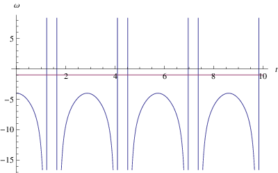
In Fig. 2, we depict the cosmological evolution of EoS as a function of for . From Fig. 2, we see that the universe always evolves within the phantom phase (). Consequently, this model is ruled out.
IV.3 MG – XIV model
We provide that the Hubble parameter is described as
| (44) |
so that the scale factor can read as
| (45) |
From Eq. (44) and the gravitational field equations (1) and (2), we have the parametric EoS
| (46) | |||||
| (47) |
Hence, the EoS parameter is written as
| (48) |
With Eqs. (33) and (34), we have
| (49) | |||||
| (50) |
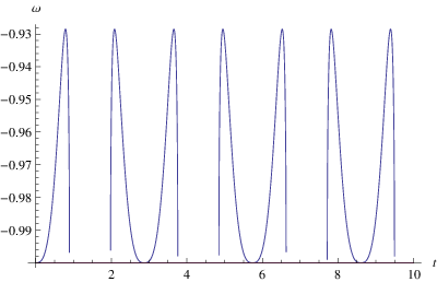
In Fig. 3, we illustrate the cosmological evolution of EoS as a function of for . From Fig. 3, we see that the universe always stays in the non-phantom (quintessence) phase ().
IV.4 MG – XV model
We take the form of the Hubble parameter as
| (51) |
From this form, the corresponding scale factor is given by
| (52) |
With Eq. (51) and the gravitational field equations (33) and (34), we obtain the parametric EoS
| (53) | |||||
| (54) |
It follows from Eqs. (53) and (54) that the parametric EoS is given by
| (55) |
By using the formulae in Eqs. (33) and (34), we acquire
| (56) | |||||
| (57) |
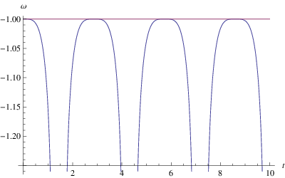
In Fig. 4, we display the cosmological evolution of EoS as a function of for . From Fig. 4, we understand that the universe always evolves within the phantom phase (). Thus, this model is ruled out.
IV.5 MG – XVI model
We assume that the Hubble parameter is written as
| (58) |
In this case, the scale factor becomes
| (59) |
Using Eq. (58) and the gravitational field equations (1) and (2) yields
| (60) | |||||
| (61) |
Hence, the parametric EoS is expressed as
| (62) |
From Eqs. (33) and (34), we acquire
| (63) | |||||
| (64) |
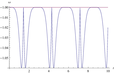
In Fig. 5, we plot the cosmological evolution of EoS as a function of for . From Fig. 5, we find that the universe always evolves within the phantom phase (). Therefore, this model is ruled out. In addition, we clearly see the two periodic oscillating evolution of .
IV.6 MG – XVII model
We take the scale factor as
| (65) |
From this expression, the Hubble parameter becomes
| (66) |
Equation (66) and the gravitational field equations (1) and (2) present the parametric EoS
| (67) | |||||
| (68) |
Furthermore, the EoS parameter is represented as
| (69) |
From Eqs. (33) and (34), we have
| (70) | |||||
| (71) |
In Fig. 6, we plot the cosmological evolution of EoS as a function of for . From Fig. 6, we see that the universe always stays in the phantom phase (). Accordingly, this model is ruled out.

IV.7 MG – XVIII model
We describe the scale factor as
| (72) |
It follows from this description that the Hubble parameter is given by
| (73) |
IV.8 MG – XIX model
We consider that the scale factor is given by
| (74) |
so that the Hubble parameter can read
| (75) |
IV.9 MG – XX model
We suppose the following form of the scale factor
| (76) |
From this representation, the Hubble parameter is written by
| (77) |
IV.10 MG – XXXIII model
We suppose that the scale factor takes the following form
| (78) |
It follows from this representation that the Hubble parameter is described by
| (79) |
It is important to mention that a quintom model (where there must exist both canonical and non-canonical scalar fields in order that the crossing of the phantom divide can occur) with single canonical scalar field cannot be reconstructed, in which the crossing of the phantom divide cannot occur [124]. Since in MG – XVIII, XIX, XX and XXXIII models explained in Sections 4.7, 4.8, 4.9 and 4.10, respectively, if we reconstruct the corresponding single scalar field model, the crossing of the phantom divide can be realized. Thus, this implies that for these models, such a reconstruction is not physical but just mathematical procedure.
The physical interpretation of our results is considered as follows. By reconstructing the expansion behavior of the universe, i.e., the Hubble parameter, with the Weierstrass -function, which has a periodic property, the periodic behavior of the EoS for the universe can be realized. Such a procedure can be applied to scenarios to avoid cosmological singularities and eventually a non-singular universe can be realized.
It is also remarkable to note that in terms of all the numerical calculations in Figs. 1–6, the qualitative results do not strongly depend on the initial conditions and the model parameters such as the Weierstrass -function.
Moreover, for all the models, the scale factor has to be positive and the Hubble parameter should be real. From Eqs. (26), (38), (45), (52) and (59), is always positive. Also, it follows from Eqs. (65), (72), (74), (76) and (78) that is written by or its time derivatives. By using the Laurent expansion of around as , we find , , , and . Thus, for the cases of in Eq. (72) and in Eq. (76), around , the expression of is not well defined because the value of would become negative around . In this sense, around , the MG – XVIII and MG – XX models cannot be used. On the other hand. since the argument of the Weierstrass functions used in this paper is the cosmic time , which is real, all the values of the Weierstrass functions are real. In all the models, is described by the Weierstrass functions and hence would be real.
Furthermore, we state that if the evolution of is displayed as a function of the redshift with the present value of , the direction of the cosmic time to go by becomes opposite to that for to be shown as a function of in Figs. 1–6. It would be considered that the main qualitative difference is only this point and hence other cosmological consequences do not change.
In addition, it is interesting to note that the models examined in this work may solve, not only the dark energy paradigm, but also the horizon and flatness problems. In other words, these models may produce a kind of inflationary epoch or perhaps a contraction phase as in the ekpyrotic scenario. In order for inflation or the ekpyrotic scenario to be realized realistically, it is necessary to consider the way of connect the inflationary stage and the dark energy dominated stage, i.e., the realization of the reheating stage. This is a crucial point for these models to be realistic inflation models or the ekpyrotic scenario.
Moreover, it should be cautioned that in Figs. 2–4, apparently it looks the EoS diverges. However, the reason is just a way of plotting and therefore there is no divergence in terms of the EoS in all of the figures.
Finally, we mention the issue of existence of a ghost, namely, the instability for the case of the crossing of the phantom divide. For a scalar field theory, it is known that if the crossing of the phantom divide happens in the FLRW universe, there would appear a ghost. In Sec. IV, we have presented the interpretations of our models in the framework of a scalar field theory. However, there still exists the possibility that our models could be regarded as a more complicated theory, e.g., which is described by the non-linear kinetic terms such as -essence models [125, 126, 127, 128, 129, 130] and the Galileon models [131, 132, 133, 134, 135]. These investigations might be one of the interesting future works in our approach to the periodic and quasi-periodic generalizations of the Chaplygin gas type models.
V Conclusions
In the present paper, we have reconstructed periodic and quasi-periodic generalizations of the Chaplygin gas type models by using the Weierstrass , and -elliptic functions. We have explored the cosmological evolution of the EoS for dark energy in FLRW spacetime. In particular, we have shown that by using the degenerate properties of the elliptic functions, the MCG models can be recovered. This is one of the most important cosmological ingredients obtained in this paper. This result implies that by plugging the reconstruction method of the expansion history of the universe with the Weierstrass elliptic functions, we can acquire the MCG models, which have a potential to reveal the properties of both dark energy and dark matter. In other words, the procedure demonstrated in this paper can lead to a preferable cosmological model by starting with the mathematical special functions.
It is meaningful to summarize the following significant points. (a) The Weierstrass functions have two periods and . This is their essential property. (b) Our periodic and quasi-periodic models given in Sec. III are periodic or quasi-periodic in terms of the energy density . (c) Furthermore, if the special values of the periods and are infinite, these models in Sec. III are transformed into or have limits of the Chaplygin gas models, which can be seen from the formulae in (3.1). Thus, in this sense to reconstruct these models is considered to be two periodic or quasi periodical generalizations of the CG models. This is the justification of application of the Weierstrass functions to cosmological models. (d) Our models presented in Sec. IV are periodic on the cosmic time (which is here dimensionless) contrast to the models in Sec. III which are periodic/quasiperiodic on . (e) Moreover, our periodic/quasiperiodic models in Sec. III are singular at and those in Sec. IV at .
It is also important to emphasize that the cosmological advantage to acquire the periodic evolution of the universe is to realize scenarios to avoid a Big Bang singularity, the finite-time future singularities and a Big Crunch singularity. By applying the obtained results and the discussed procedure to scenarios for the avoidance of singularities, e.g., the cyclic universe, the ekpyrotic scenario and the bouncing universe, we can find a non-singular cosmology.
Furthermore, it has explicitly been illustrated that there are three type models with realizing the cosmological evolution of the EoS for dark energy : (i) The universe always stays in the non-phantom (quintessence) phase (the MG – XIV model). (ii) The universe always evolves within the phantom phase (the MG – XII, MG – XIII, MG – XV, MG – XVI and MG – XVII models). (iii) The crossing of the phantom divide can be realized (the MG – XVIII, MG – XIX, MG – XX and MG – XXXIII models). If the universe always stays in the phantom phase, it is impossible to describe the whole evolution history of the universe, i.e., the decelerated phases such as the radiation and matter dominated stages. Thus, these models are ruled out. In addition, the corresponding description of a canonical scalar field model to the models in the above (iii) category is not physical but just mathematical because in the light of quintom model [124], it is impossible for a single canonical scalar field to realize the crossing of the phantom divide.
The scalar fields and the corresponding potentials have been analyzed for different types of MG models mentioned above. The EoS parameters have been derived and their natures have also been illustrated graphically during the evolution of the universe.
On the other hand, at the current stage the cosmological constant is consistent with the observational data [4], but there still exists the possibility of dynamical dark energy, which is, e.g., described by a scalar field or a fluid. Thus, when we acquire the results of data analysis of the more precise future experiments like by the PLANCK satellite [136], it is strongly expected that the investigations on the phase of the universe, i.e., the non-phantom or phantom phase, or the crossing of the phantom divide can become more meaningful. In the future work, it would be interesting that whether the above models may be suitable candidates for dark energy is tested by coming observational data fittings.
Acknowledgments
K.B. would like to sincerely acknowledge very kind and warm hospitality at Eurasian National University very much, where this work has been completed. In addition, he is grateful to National Center for Theoretical Sciences and National Tsing Hua University very much for the very kind and warm hospitality, where the revision of this work was executed.
References
- [1] D. N. Spergel et al. [WMAP Collaboration], Astrophys. J. Suppl. 148, 175 (2003) [arXiv:astro-ph/0302209].
- [2] D. N. Spergel et al. [WMAP Collaboration], Astrophys. J. Suppl. 170, 377 (2007) [arXiv:astro-ph/0603449].
- [3] E. Komatsu et al. [WMAP Collaboration], Astrophys. J. Suppl. 180, 330 (2009) [arXiv:0803.0547 [astro-ph]].
- [4] E. Komatsu et al. [WMAP Collaboration], Astrophys. J. Suppl. 192, 18 (2011) [arXiv:1001.4538 [astro-ph.CO]].
- [5] S. Perlmutter et al. [SNCP Collaboration], Astrophys. J. 517, 565 (1999) [arXiv:astro-ph/9812133].
- [6] A. G. Riess et al. [Supernova Search Team Collaboration], Astron. J. 116, 1009 (1998) [arXiv:astro-ph/9805201].
- [7] M. Tegmark et al. [SDSS Collaboration], Phys. Rev. D 69, 103501 (2004) [arXiv:astro-ph/0310723].
- [8] U. Seljak et al. [SDSS Collaboration], Phys. Rev. D 71, 103515 (2005) [arXiv:astro-ph/0407372].
- [9] D. J. Eisenstein et al. [SDSS Collaboration], Astrophys. J. 633, 560 (2005) [arXiv:astro-ph/0501171].
- [10] B. Jain and A. Taylor, Phys. Rev. Lett. 91, 141302 (2003) [arXiv:astro-ph/0306046].
- [11] E. J. Copeland, M. Sami and S. Tsujikawa, Int. J. Mod. Phys. D 15, 1753 (2006) [arXiv:hep-th/0603057].
- [12] R. Durrer and R. Maartens, Gen. Rel. Grav. 40, 301 (2008) [arXiv:0711.0077 [astro-ph]].
- [13] R. Durrer and R. Maartens, arXiv:0811.4132 [astro-ph].
- [14] Y. F. Cai, E. N. Saridakis, M. R. Setare and J. Q. Xia, Phys. Rept. 493, 1 (2010) [arXiv:0909.2776 [hep-th]].
- [15] S. Tsujikawa, arXiv:1004.1493 [astro-ph.CO].
- [16] L. Amendola and S. Tsujikawa, Dark Energy (Cambridge University press, 2010).
- [17] M. Li, X. D. Li, S. Wang and Y. Wang, Commun. Theor. Phys. 56, 525 (2011) [arXiv:1103.5870 [astro-ph.CO]].
- [18] K. Bamba, S. Capozziello, S. Nojiri and S. D. Odintsov, Astrophys. Space Sci. 342, 155 (2012) [arXiv:1205.3421 [gr-qc]].
- [19] S. Nojiri and S. D. Odintsov, Phys. Rept. 505, 59 (2011) [arXiv:1011.0544 [gr-qc]].
- [20] S. Nojiri and S. D. Odintsov, eConf C0602061, 06 (2006) [Int. J. Geom. Meth. Mod. Phys. 4, 115 (2007)] [arXiv:hep-th/0601213].
- [21] T. P. Sotiriou and V. Faraoni, Rev. Mod. Phys. 82, 451 (2010) [arXiv:0805.1726 [gr-qc]].
- [22] S. Capozziello and V. Faraoni, Beyond Einstein Gravity (Springer, 2010).
- [23] S. Capozziello and M. De Laurentis, Phys. Rept. 509, 167 (2011) [arXiv:1108.6266 [gr-qc]].
- [24] A. De Felice and S. Tsujikawa, Living Rev. Rel. 13, 3 (2010) [arXiv:1002.4928 [gr-qc]].
- [25] T. Clifton, P. G. Ferreira, A. Padilla and C. Skordis, Phys. Rept. 513, 1 (2012) [arXiv:1106.2476 [astro-ph.CO]].
- [26] S. Capozziello, M. De Laurentis and S. D. Odintsov, Eur. Phys. J. C 72, 2068 (2012) [arXiv:1206.4842 [gr-qc]].
- [27] R. R. Caldwell, M. Kamionkowski and N. N. Weinberg, Phys. Rev. Lett. 91, 071301 (2003) [arXiv:astro-ph/0302506].
- [28] B. McInnes, JHEP 0208 (2002) 029 [arXiv:hep-th/0112066].
- [29] S. Nojiri and S. D. Odintsov, Phys. Lett. B 562, 147 (2003) [arXiv:hep-th/0303117].
- [30] S. Nojiri and S. D. Odintsov, Phys. Lett. B 571, 1 (2003) [arXiv:hep-th/0306212].
- [31] V. Faraoni, Int. J. Mod. Phys. D 11, 471 (2002) [arXiv:astro-ph/0110067].
- [32] P. F. Gonzalez-Diaz, Phys. Lett. B 586, 1 (2004) [arXiv:astro-ph/0312579].
- [33] E. Elizalde, S. Nojiri and S. D. Odintsov, Phys. Rev. D 70, 043539 (2004) [arXiv:hep-th/0405034].
- [34] P. Singh, M. Sami and N. Dadhich, Phys. Rev. D 68, 023522 (2003) [arXiv:hep-th/0305110].
- [35] C. Csaki, N. Kaloper and J. Terning, Annals Phys. 317, 410 (2005) [arXiv:astro-ph/0409596].
- [36] P. X. Wu and H. W. Yu, Nucl. Phys. B 727, 355 (2005) [arXiv:astro-ph/0407424].
- [37] S. Nesseris and L. Perivolaropoulos, Phys. Rev. D 70, 123529 (2004) [arXiv:astro-ph/0410309].
- [38] M. Sami and A. Toporensky, Mod. Phys. Lett. A 19, 1509 (2004) [arXiv:gr-qc/0312009].
- [39] H. Stefancic, Phys. Lett. B 586, 5 (2004) [arXiv:astro-ph/0310904].
- [40] L. P. Chimento and R. Lazkoz, Phys. Rev. Lett. 91, 211301 (2003) [arXiv:gr-qc/0307111].
- [41] J. G. Hao and X. Z. Li, Phys. Lett. B 606, 7 (2005) [arXiv:astro-ph/0404154].
- [42] E. Elizalde, S. Nojiri, S. D. Odintsov and P. Wang, Phys. Rev. D 71, 103504 (2005) [arXiv:hep-th/0502082].
- [43] M. P. Dabrowski and T. Stachowiak, Annals Phys. 321, 771 (2006) [arXiv:hep-th/0411199].
- [44] F. S. N. Lobo, Phys. Rev. D 71, 084011 (2005) [arXiv:gr-qc/0502099].
- [45] R. G. Cai, H. S. Zhang and A. Wang, Commun. Theor. Phys. 44, 948 (2005) [arXiv:hep-th/0505186].
- [46] I. Y. Aref’eva, A. S. Koshelev and S. Y. Vernov, Phys. Rev. D 72, 064017 (2005) [arXiv:astro-ph/0507067].
- [47] H. Q. Lu, Z. G. Huang and W. Fang, arXiv:hep-th/0504038.
- [48] W. Godlowski and M. Szydlowski, Phys. Lett. B 623, 10 (2005) [arXiv:astro-ph/0507322].
- [49] J. Sola and H. Stefancic, Phys. Lett. B 624, 147 (2005) [arXiv:astro-ph/0505133].
- [50] B. Guberina, R. Horvat and H. Nikolic, Phys. Rev. D 72, 125011 (2005) [arXiv:astro-ph/0507666].
- [51] Y. Shtanov and V. Sahni, Class. Quant. Grav. 19, L101 (2002) [arXiv:gr-qc/0204040].
- [52] J. D. Barrow, Class. Quant. Grav. 21, L79 (2004) [arXiv:gr-qc/0403084].
- [53] S. Nojiri and S. D. Odintsov, Phys. Lett. B 595, 1 (2004) [arXiv:hep-th/0405078].
- [54] S. Nojiri and S. D. Odintsov, Phys. Rev. D 70, 103522 (2004) [arXiv:hep-th/0408170].
- [55] S. Nojiri and S. D. Odintsov, Phys. Rev. D 72, 023003 (2005) [arXiv:hep-th/0505215].
- [56] S. Cotsakis and I. Klaoudatou, J. Geom. Phys. 55, 306 (2005) [arXiv:gr-qc/0409022].
- [57] M. P. Dabrowski, Phys. Rev. D 71, 103505 (2005) [arXiv:gr-qc/0410033].
- [58] L. Fernandez-Jambrina and R. Lazkoz, Phys. Rev. D 70, 121503 (2004) [arXiv:gr-qc/0410124].
- [59] L. Fernandez-Jambrina and R. Lazkoz, Phys. Lett. B 670, 254 (2009) [arXiv:0805.2284 [gr-qc]].
- [60] J. D. Barrow and C. G. Tsagas, Class. Quant. Grav. 22, 1563 (2005) [arXiv:gr-qc/0411045].
- [61] H. Stefancic, Phys. Rev. D 71, 084024 (2005) [arXiv:astro-ph/0411630].
- [62] C. Cattoen and M. Visser, Class. Quant. Grav. 22, 4913 (2005) [arXiv:gr-qc/0508045].
- [63] P. Tretyakov, A. Toporensky, Y. Shtanov and V. Sahni, Class. Quant. Grav. 23, 3259 (2006) [arXiv:gr-qc/0510104].
- [64] A. Balcerzak and M. P. Dabrowski, Phys. Rev. D 73, 101301 (2006) [arXiv:hep-th/0604034].
- [65] M. Sami, P. Singh and S. Tsujikawa, Phys. Rev. D 74, 043514 (2006) [arXiv:gr-qc/0605113].
- [66] M. Bouhmadi-Lopez, P. F. Gonzalez-Diaz and P. Martin-Moruno, Phys. Lett. B 659, 1 (2008) [arXiv:gr-qc/0612135].
- [67] A. V. Yurov, A. V. Astashenok and P. F. Gonzalez-Diaz, Grav. Cosmol. 14, 205 (2008) [arXiv:0705.4108 [astro-ph]].
- [68] T. Koivisto, Phys. Rev. D 77, 123513 (2008) [arXiv:0803.3399 [gr-qc]].
- [69] J. D. Barrow and S. Z. W. Lip, Phys. Rev. D 80, 043518 (2009) [arXiv:0901.1626 [gr-qc]].
- [70] M. Bouhmadi-Lopez, Y. Tavakoli and P. V. Moniz, JCAP 1004, 016 (2010) [arXiv:0911.1428 [gr-qc]].
- [71] S. Nojiri, S. D. Odintsov and S. Tsujikawa, Phys. Rev. D 71 (2005) 063004 [arXiv:hep-th/0501025].
- [72] S. Nojiri and S. D. Odintsov, Phys. Rev. D 78, 046006 (2008) [arXiv:0804.3519 [hep-th]].
- [73] K. Bamba, S. Nojiri and S. D. Odintsov, JCAP 0810 (2008) 045 [arXiv:0807.2575 [hep-th]].
- [74] K. Bamba, S. D. Odintsov, L. Sebastiani and S. Zerbini, Eur. Phys. J. C 67 (2010) 295 [arXiv:0911.4390 [hep-th]].
- [75] P. J. Steinhardt and N. Turok, Phys. Rev. D 65, 126003 (2002) [arXiv:hep-th/0111098].
- [76] P. J. Steinhardt and N. Turok, [arXiv:hep-th/0111030].
- [77] J. Khoury, B. A. Ovrut, P. J. Steinhardt and N. Turok, Phys. Rev. D 66, 046005 (2002) [arXiv:hep-th/0109050].
- [78] P. J. Steinhardt and N. Turok, Nucl. Phys. Proc. Suppl. 124, 38 (2003) [arXiv:astro-ph/0204479].
- [79] P. J. Steinhardt and N. Turok, Science 296, 1436 (2002).
- [80] J. Khoury, P. J. Steinhardt and N. Turok, Phys. Rev. Lett. 92, 031302 (2004) [arXiv:hep-th/0307132].
- [81] P. J. Steinhardt and N. Turok, Science 312, 1180 (2006) [astro-ph/0605173].
- [82] K. Saaidi, H. Sheikhahmadi and A. H. Mohammadi, Astrophys. Space Sci. 338, 355 (2012) [arXiv:1201.0275 [gr-qc]].
- [83] S. Nojiri, S. D. Odintsov and D. Saez-Gomez, AIP Conf. Proc. 1458, 207 (2011) [arXiv:1108.0767 [hep-th]].
- [84] Y. F. Cai and E. N. Saridakis, J. Cosmol. 17, 7238 (2011) [arXiv:1108.6052 [gr-qc]].
- [85] V. Sahni and A. Toporensky, Phys. Rev. D 85, 123542 (2012) [arXiv:1203.0395 [gr-qc]].
- [86] D. Y. Chung, arXiv:physics/0105064.
- [87] J. Khoury, B. A. Ovrut, P. J. Steinhardt and N. Turok, Phys. Rev. D 64, 123522 (2001) [arXiv:hep-th/0103239].
- [88] J. Khoury, B. A. Ovrut, P. J. Steinhardt and N. Turok, arXiv:hep-th/0105212.
- [89] R. Y. Donagi, J. Khoury, B. A. Ovrut, P. J. Steinhardt and N. Turok, JHEP 0111, 041 (2001) [arXiv:hep-th/0105199].
- [90] D. N. Page, Class. Quant. Grav. 1, 417 (1984).
- [91] P. Peter and N. Pinto-Neto, Phys. Rev. D 65, 023513 (2001) [arXiv:gr-qc/0109038].
- [92] P. Peter and N. Pinto-Neto, Phys. Rev. D 66, 063509 (2002) [arXiv:hep-th/0203013].
- [93] Y. Shtanov and V. Sahni, Phys. Lett. B 557, 1 (2003) [arXiv:gr-qc/0208047].
- [94] T. Biswas, A. Mazumdar and W. Siegel, JCAP 0603, 009 (2006) [arXiv:hep-th/0508194].
- [95] Y. F. Cai, T. Qiu, Y. S. Piao, M. Li and X. Zhang, JHEP 0710, 071 (2007) [arXiv:0704.1090 [gr-qc]].
- [96] P. Creminelli and L. Senatore, JCAP 0711, 010 (2007) [arXiv:hep-th/0702165].
- [97] Y. S. Piao, Phys. Lett. B 677, 1 (2009) [arXiv:0901.2644 [gr-qc]].
- [98] J. Zhang, Z. G. Liu and Y. S. Piao, Phys. Rev. D 82, 123505 (2010) [arXiv:1007.2498 [hep-th]].
- [99] Y. S. Piao, Phys. Lett. B 691, 225 (2010) [arXiv:1001.0631 [hep-th]].
- [100] Z. G. Liu and Y. S. Piao, Phys. Rev. D 86, 083510 (2012) [arXiv:1201.1371 [gr-qc]].
- [101] M. Novello and S. E. P. Bergliaffa, Phys. Rept. 463, 127 (2008) [arXiv:0802.1634 [astro-ph]].
- [102] R. Myrzakulov, to appear in Gen. Rel. Grav. DOI: 10.1007/s10714-012-1439-z, arXiv:1008.4486 [physics.gen-ph].
- [103] R. Myrzakulov, Advances in High Energy Physics, 2012, 868203 (2012) [arXiv:1204.1093 [physics.gen-ph]].
- [104] K. Esmakhanova, Y. Myrzakulov, G. Nugmanova and R. Myrzakulov, Int. J. Theor. Phys. 51, 1204 (2012) [arXiv:1102.4456 [physics.gen-ph]].
- [105] K. R. Yesmakhanova, N. A. Myrzakulov, K. K. Yerzhanov, G. N. Nugmanova, N. S. Serikbayaev and R. Myrzakulov, arXiv:1201.4360 [physics.gen-ph].
- [106] G. W. Gibbons and M. Vyska, Class. Quant. Grav. 29, 065016 (2012) [arXiv:1110.6508 [gr-qc]].
- [107] I. Bochicchio, S. Capozziello and E. Laserra, Int. J. Geom. Meth. Mod. Phys. 8, 1653 (2011) [arXiv:1111.0819 [gr-qc]].
- [108] B. G. Dimitrov, J. Math. Phys. 44, 2542 (2003) [arXiv:hep-th/0107231].
- [109] J. D’Ambroise, arXiv:0908.2481 [gr-qc].
- [110] M. Bouhmadi-Lopez, L. J. Garay and P. F. Gonzalez-Diaz, Phys. Rev. D 66, 083504 (2002) [arXiv:gr-qc/0204072].
- [111] K. Bamba, K. Yesmakhanova, K. Yerzhanov and R. Myrzakulov, arXiv:1203.3401 [gr-qc].
- [112] A. Y. Kamenshchik, U. Moschella and V. Pasquier, Phys. Lett. B 511 (2001) 265 [arXiv:gr-qc/0103004].
- [113] M. C. Bento, O. Bertolami and A. A. Sen, Phys. Rev. D 66 (2002) 043507 [arXiv:gr-qc/0202064].
- [114] H. B. Benaoum, arXiv:hep-th/0205140.
- [115] D. Saez-Gomez, Grav. Cosmol. 15, 134 (2009) [arXiv:0804.4586 [hep-th]].
- [116] M. Sharif, K. Yesmakhanova, S. Rani and R. Myrzakulov, Eur. Phys. J. C 72, 2067 (2012) [arXiv:1204.2181 [physics.gen-ph]].
- [117] K. Bamba, S. Nojiri, S. D. Odintsov and M. Sasaki, Gen. Rel. Grav. 44, 1321 (2012) [arXiv:1104.2692 [hep-th]].
- [118] U. Alam, V. Sahni and A. A. Starobinsky, JCAP 0406, 008 (2004) [arXiv:astro-ph/0403687].
- [119] U. Alam, V. Sahni and A. A. Starobinsky, JCAP 0702, 011 (2007) [arXiv:astro-ph/0612381].
- [120] S. Nesseris and L. Perivolaropoulos, JCAP 0701, 018 (2007) [arXiv:astro-ph/0610092].
- [121] P. U. Wu and H. W. Yu, Phys. Lett. B 643, 315 (2006) [arXiv:astro-ph/0611507].
- [122] H. K. Jassal, J. S. Bagla and T. Padmanabhan, Mon. Not. Roy. Astron. Soc. 405, 2639 (2010) [arXiv:astro-ph/0601389].
- [123] Handbook of Mathematical Functions with Formulas, Graphs, and Mathematical Tables (1964), edited by M. Abramowitz and l. A. Stegun.
- [124] G. -B. Zhao, J. -Q. Xia, M. Li, B. Feng and X. Zhang, Phys. Rev. D 72, 123515 (2005) [astro-ph/0507482].
- [125] T. Chiba, T. Okabe and M. Yamaguchi, Phys. Rev. D 62, 023511 (2000) [arXiv:astro-ph/9912463].
- [126] C. Armendariz-Picon, T. Damour and V. F. Mukhanov, Phys. Lett. B 458, 209 (1999) [arXiv:hep-th/9904075].
- [127] J. Garriga and V. F. Mukhanov, Phys. Lett. B 458, 219 (1999) [arXiv:hep-th/9904176].
- [128] C. Armendariz-Picon, V. F. Mukhanov and P. J. Steinhardt, Phys. Rev. Lett. 85, 4438 (2000) [arXiv:astro-ph/0004134].
- [129] C. Armendariz-Picon, V. F. Mukhanov and P. J. Steinhardt, Phys. Rev. D 63, 103510 (2001) [arXiv:astro-ph/0006373].
- [130] R. de Putter and E. V. Linder, Astropart. Phys. 28, 263 (2007) [arXiv:0705.0400 [astro-ph]].
- [131] A. Nicolis, R. Rattazzi and E. Trincherini, Phys. Rev. D 79, 064036 (2009) [arXiv:0811.2197 [hep-th]].
- [132] C. Deffayet, G. Esposito-Farese and A. Vikman, Phys. Rev. D 79, 084003 (2009) [arXiv:0901.1314 [hep-th]].
- [133] C. Deffayet, S. Deser and G. Esposito-Farese, Phys. Rev. D 80, 064015 (2009) [arXiv:0906.1967 [gr-qc]].
- [134] C. Deffayet, S. Deser and G. Esposito-Farese, Phys. Rev. D 82, 061501 (2010) [arXiv:1007.5278 [gr-qc]].
- [135] N. Shirai, K. Bamba, S. Kumekawa, J. Matsumoto and S. Nojiri, Phys. Rev. D 86, 043006 (2012) [arXiv:1203.4962 [hep-th]].
- [136] http://www.sciops.esa.int/index.php?project=PLANCK.