Higgs Physics: Theory

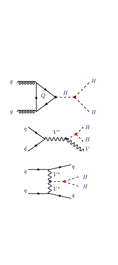
There are essentially four mechanisms for the single production of the SM Higgs boson at hadron colliders; some Feynman diagrams are shown in Fig. 1.

The total production cross sections, borrowed from Refs [19, 20] and obtained using adapted versions of the programs of Ref. [21], are displayed in Fig. 2 for the Tevatron with $\sqrt{s}=1.96$ TeV and the LHC with $\sqrt{s}=7$ TeV as a function of the Higgs mass; the top quark mass is set to $m_{t}=173.1$ GeV [6] and the MSTW [22] parton distributions functions (PDFs) have been adopted. The most important higher order QCD and electroweak corrections, summarized below for each production channel, have been implemented .

The gluon–gluon fusion process $gg\to H$ is by far the dominant production channel for SM–like Higgs particles at hadron colliders. The process, which proceeds through triangular heavy quark loops, has been proposed in the late 1970s in Ref. [23] where the $ggH$ vertex and the production cross section have been derived. In the SM, it is dominantly mediated by the top quark loop contribution, while the bottom quark contribution does not exceed the 10% level at leading order. This process is known to be subject to extremely large QCD radiative corrections that can be described by an associated $K$–factor defined as the ratio of the higher order (HO) to the lowest order (LO) cross sections, consistently evaluated with the value of the strong coupling $\alpha_{s}$ and the parton distribution functions taken at the considered perturbative order.

The next-to-leading-order (NLO) corrections in QCD have been calculated in the 1990s. They are known both for infinite [24] and finite [25, 26] loop quark masses and, at the $\sqrt{s}\!=\!7$ TeV LHC, lead to a $K$–factor $K_{\rm NLO}\sim 1.8$ in the low Higgs mass range, if the central scale of the cross section is chosen to be $M_{H}$. It has been shown in Ref. [26] that working in an effective field theory (EFT) approach in which the top quark mass is assumed to be infinite is a very good approximation for $M_{H}\raisebox{-3.69899pt}{~\shortstack{$<$ \\ [-0.07cm] $\sim$}}~2m_{t}$, provided that the leading order cross section contains the full $m_{t}$ and $m_{b}$ dependence. The challenging calculation of the next-to-next-to-leading-order (NNLO) contribution has been done [27] only in the EFT approach with $M_{H}\ll 2m_{t}$ and, at $\sqrt{s}=7$ TeV, it leads to a $\approx 25\%$ increase of the cross section, $K_{\rm NNLO}\sim 2.5$. The resummation of soft gluons is known up to next-to-next-to-leading-logarithm (NNLL) and, again, increases the cross section by slightly less than 10% [28, 29]. The effects of soft–gluon resumation at NNLL can be accounted for in $\sigma^{\rm NNLO}(gg\to H)$ by lowering the central value of the renormalization and factorization scales, from $\mu_{0}\!=\!\mu_{R}\!=\!\mu_{F}\!=\!M_{H}$ to $\mu_{0}\!=\!\frac{1}{2}M_{H}$; see e.g. Ref. [30]. The latter value is chosen for the cross section at NNLO displayed in Fig. 2. Note in passing that the choice $\mu_{0}=\frac{1}{2}M_{H}$ also improves the convergence of the perturbative series and is more appropriate to describe the kinematics of the process. Some small additional corrections beyond NNLO have been also calculated [31, 32, 33]. The electroweak corrections are known both in some approximations [34] and exactly at NLO [35] and contribute at the level of a few percent; there are also small mixed NNLO QCD–electroweak effects which have been calculated in an effective approach valid for $M_{H}\ll M_{W}$ [30].

The QCD corrections to $gg\to H$ at $\sqrt{s}=7$ TeV are smaller than the corresponding ones at the Tevatron as the $K$–factors in this case are $K_{\rm NLO}\approx 2$ and $K_{\rm NNLO}\approx 3$ (with again a central scale equal to $M_{H}$). In turn, at the LHC with $\sqrt{s}=14$ TeV, the $K$–factors are smaller, $K_{\rm NLO}\approx 1.7$ and $K_{\rm NNLO}\approx 2$. The perturbative series shows thus a better (converging) behavior at LHC than at Tevatron energies. The impact of all these QCD corrections is summarized in Fig. 3 for the LHC at $\sqrt{s}=14$ TeV and for the Tevatron. Updates of the Higgs cross sections including the relevant higher order corrections have been performed in various recent papers, see e.g. Refs. [29, 30, 19, 20, 36, 37].

Note that the QCD corrections to the differential distributions, and in particular to the Higgs transverse momentum and rapidity distributions, have also been calculated at NLO (with a resummation for the former) and shown to be in general rather large; see Ref. [38] for an account. These calculations are implemented in several programs [39] which allow to derive the full differential cross section and hence the $gg\!\to\!H$ cross section with cuts.

Let us now briefly discuss the other Higgs production processes at hadron colliders.

The Higgs–strahlung processes where the Higgs is produced in association with $V=W,Z$ bosons, $q\bar{q}\to HV$ [40], are known exactly up to NNLO in QCD [41, 42, 43] (at NLO it can be inferred from Drell–Yan production) and up to NLO for the electroweak corrections [44]. In Fig. 2, the corrections are evaluated at a central scale $\mu_{0}=M_{HV}$, i.e. the invariant mass of the $HV$ system. Here, the QCD $K$–factors are moderate both at the Tevatron and the LHC, $K_{\rm NNLO}\sim 1.5$ and the electroweak corrections reduce the cross section by a few percent. The remaining scale dependence is very small, making this process the theoretically cleanest of all Higgs production processes. Note that the differential cross section is also known up to NNLO; see for instance Ref. [45].

The vector boson fusion channel, where the Higgs is produced in association with two jets, $qq\to Hqq$ [46], is the second most important process at the LHC. The QCD corrections, which can be obtained in the structure–function approach, are moderate at NLO being at the level of 10% [47, 42]. The NNLO corrections which have been calculated recently have been found to be very small [48]. The electroweak corrections have been derived in Ref. [49]. The corrections including cuts, and in particular corrections to the transverse momentum and rapidity distributions, have also been calculated and implemented into a parton–level Monte–Carlo programs such as in Ref. [50].

Finally, there is associated Higgs production with top quark pairs [51] which is only relevant at the LHC. The cross section is rather involved at tree–level since it is a three–body process, and the calculation of the NLO corrections was a real challenge which was met a few years ago [52]. The $K$–factors turned out to be rather small, $K\sim 1.2$ and $K\sim 1$ at the LHC with, respectively, $\sqrt{s}=14$ TeV and 7 TeV ($K\sim 0.8$ at the Tevatron) if the central scale is chosen to be $\mu_{0}\!=\!\frac{1}{2}(M_{H}+2m_{t})$. However, the scale dependence is drastically reduced from a factor two at LO to the level of 10–20% at NLO.

Note that there are also other Higgs production processes at hadron colliders but which are of higher perturbative order. For instance double Higgs production, which is sensitive to the Higgs self–coupling, can be produced in various processes such as $gg\to HH$, but with rather low cross sections at the LHC as will be discussed later.

It is well known that the production cross sections at hadron colliders as well as the associated kinematical distributions are generally affected by various theoretical uncertainties. In the case of the gluon–gluon fusion channel, these theoretical uncertainties turn out to be particularly large. They are stemming from three main sources.

First, the perturbative QCD corrections to the $gg\to H$ cross section are so large that one may question the reliability of the perturbative series (in particular, at the Tevatron as discussed above) and the possibility of still large higher order contributions beyond NNLO cannot be excluded. The effects of the unknown contributions are usually estimated from the variation of the cross section with the renormalisation $\mu_{R}$ and factorisation $\mu_{F}$ scales at which the process is evaluated. Starting from a median scale taken to be $\mu_{R}\!=\!\mu_{F}\!=\!\mu_{0}\!=\!\frac{1}{2}M_{H}$ in the $gg\!\to\!H$ process, the current convention is to vary these two scales within the range $\mu_{0}/\kappa\!\leq\!\mu_{R},\mu_{F}\!\leq\!\kappa\mu_{0}$ with the choice $\kappa\!=\!2$. This leads to a $\approx\pm 10\%$ uncertainty at the 7 TeV LHC [36, 20] as can be seen in Fig. 4 (left).

Another problem that is specific to the $gg\to H$ process is that, already at LO, it occurs at the one–loop level with the additional complication of having to account for the finite mass of the loop particle. This renders the NLO calculation extremely complicated and the NNLO calculation a formidable task. Luckily, one can work in an effective field theory (EFT) approach in which the heavy loop particles are integrated out, making the calculation of the contributions beyond NLO possible. While this approach is justified for the dominant top quark contribution for $M_{H}\!\raisebox{-3.69899pt}{~\shortstack{$<$ \\ [-0.07cm] $\sim$}}~\!2m_{t}$ [33], it is not valid for the $b$-quark loop and for those involving the electroweak gauge bosons [34]. The uncertainties induced by the use of the EFT approach at NNLO are estimated to be of ${\cal O}(5\%)$ [20].

A third problem is due to the presently not satisfactory determination of the parton distribution functions (PDFs). Indeed, in this $gg$ initiated process, the gluon densities are poorly constrained, in particular in the high Bjorken–$x$ regime (which is particularly relevant for the Tevatron). Furthermore, since $\sigma^{\rm LO}_{gg\!\to\!H}\propto\alpha_{s}^{2}$ and receives large contributions at ${\cal O}(\geq\alpha_{s}^{3})$, a small change of $\alpha_{s}$ leads to a large variation of $\sigma^{\rm NNLO}_{gg\to H}$. Related to that is the significant difference between the world average $\alpha_{s}$ value and the one from deep-inelastic scattering (DIS) data used in the PDFs [6]. There is a statistical method to estimate the PDF uncertainties by allowing a 1$\sigma$ (or more) excursion of the experimental data that are used to perform the global fits. In addition, the MSTW collaboration [22] provides a scheme that allows for a combined evaluation of the PDF uncertainties and the (experimental and theoretical) ones on $\alpha_{s}$. In Ref. [20], the combined 90% CL PDF+$\Delta^{\rm exp}\alpha_{s}+\Delta^{\rm th}\alpha_{s}$ uncertainty on $\sigma_{gg\to H}^{\rm NNLO}$ at the 7 TeV LHC was found to be of order 10%. However, this method does not account for the theoretical assumptions that enter into the parametrization of the PDFs; a way to access this theoretical uncertainty is to compare the results for the central values of the cross section with the best–fit PDFs when using different parameterizations [53] as shown in the right panel of Fig. 4.

An important issue is the way these various uncertainties should be combined. As advocated in Refs. [20, 36], one should be conservative and add all these uncertainties linearly (this is equivalent of assuming that the PDF uncertainty is a pure theoretical uncertainty with a flat prior). In the mass range below $M_{H}\raisebox{-3.69899pt}{~\shortstack{$<$ \\ [-0.07cm] $\sim$}}~200$ GeV, this would lead to an uncertainty of about 20–25% on $\sigma^{\rm NNLO}_{gg\to H}$ as exemplified in the left-hand side of Fig. 5.

In the case of the three other Higgs production channels, because the QCD corrections are moderate, the theoretical uncertainties are much smaller: at the LHC with $\sqrt{s}=7$ TeV, they are at level of $\approx 5\%$ for the Higgs–strahlung and vector boson fusion processes and $\approx 15\%$ in the case of $t\bar{t}H$ production as exemplified in the right–hand side of Fig. 5.

Note that at the Tevatron where the QCD corrections in the $gg\to H$ process are larger than at the LHC, it is wise to extend the domain of scale variation and adopt instead a value $\kappa\!=\!3$. This is the choice made in Ref. [19] which resulted in a ${\cal O}(20\%)$ scale uncertainty. In addition, because one is in a higher Borjken–$x$ region at the Tevatron, the gluon density is less constrained and the PDF uncertainty is also larger than at the LHC. The total theoretical uncertainty on $\sigma_{gg\to H}^{\rm NNLO}$ at the Tevatron is estimated to be twice as large as at the LHC [19]. In turn, for the Higgs–strahlung process, it is of ${\cal O}(5\%)$ only.

Once its mass is fixed the profile of the Higgs particle is uniquely determined and its production rates and decay widths are fixed. As its couplings to different particles are proportional to their masses, the Higgs boson will have the tendency to decay into the heaviest particles allowed by phase space. The Higgs decay modes and their branching ratios are briefly summarized below.

In the “low–mass” range, $M_{H}\raisebox{-3.69899pt}{~\shortstack{$<$ \\ [-0.07cm] $\sim$}}~130$ GeV, the Higgs boson decays into a large variety of channels. The main mode is by far the decay into $b\bar{b}$ with a $\sim$ 60–90% probability followed by the decays into $c\bar{c}$ and $\tau^{+}\tau^{-}$ with $\sim$ 5% branching ratios. Also of significance is the top–loop mediated decay into gluons, which occurs at the level of $\sim$ 5%. The top and $W$–loop mediated $\gamma\gamma$ and $Z\gamma$ decay modes, which lead to clear signals, are very rare with rates of ${\cal O}(10^{-3})$. Note that for Higgs masses around 135 GeV, the decay $H\to WW^{*}\to Wf\bar{f}$ although at the three–body level starts to dominate over the two–body $H\to b\bar{b}$ mode: the much larger $HWW$ coupling compared to $Hb\bar{b}$ compensates for the suppression by the additional electroweak coupling and the virtuality of the $W$ boson.

In the “high–mass” range, $M_{H}\raisebox{-3.69899pt}{~\shortstack{$>$ \\ [-0.07cm] $\sim$}}~140$ GeV, the Higgs bosons decay into $WW$ and $ZZ$ pairs, one of the gauge bosons being possibly virtual below the thresholds. Above the $ZZ$ threshold, the branching ratios are 2/3 for $WW$ and 1/3 for $ZZ$ decays, and the opening of the $t\bar{t}$ channel for higher $M_{H}$ does not alter this pattern significantly.

In the low–mass range, the Higgs is very narrow, with $\Gamma_{H}<10$ MeV, but this width increases, reaching 1 GeV at the $ZZ$ threshold. For very large masses, the Higgs becomes obese, since $\Gamma_{H}\sim M_{H}$, and can hardly be considered as a resonance.

The branching ratios and total decay widths are summarized in Fig. 6, which is obtained from a recently updated version of the Fortran code HDECAY [54] which includes all relevant channels with the important radiative corrections and other higher order effects [55]. In addition, the theoretical uncertainties on the Higgs branching ratios should also be considered. Indeed, while the Higgs decays into lepton and gauge boson pairs are well under control (as mainly small electroweak effects are involved), the partial decays widths into quark pairs and gluons are plagued with uncertainties that are mainly due to the imperfect knowledge of the bottom and charm quark masses and the value of the strong coupling constant $\alpha_{s}$. At least in the intermediate mass range, $M_{H}\approx 120$–150 GeV where the SM Higgs decay rates into $b\bar{b}$ and $W^{+}W^{-}$ final states have the same order of magnitude, the parametric uncertainties on these two main Higgs decay branching ratios are non–negligible, being of the order of 3 to 10% [20, 56].

From the previous discussion, one concludes that producing the SM Higgs particle is relatively easy; this is particularly the case at the LHC thanks to the high energy of the collider and its expected luminosity. However, detecting the particle in a very complex hadronic environment is another story. Indeed, in the main Higgs decay channels the backgrounds are simply gigantic [57]. For instance, the rate for the production of light quarks and gluons is ten orders of magnitude larger than that of the Higgs boson. Even the cross sections for the production of $W$ and $Z$ bosons are three to four orders of magnitude larger. Detecting the Higgs particle is this hostile environment resembles to finding a needle in a (million) haystack, the challenges to be met being simply enormous.

To be able to detect the Higgs particle, one should take advantage in an optimal manner of the kinematical characteristics of the signal events which are, in general, quite different from that of the background events. In addition, one should focus on the decay modes of the Higgs particles (and those of the particles that are produced in association such as $W^{\pm},Z$ bosons or top quarks) that are easier to extract from the background events. Pure hadronic modes such as Higgs decays into light quark or gluon jets have to be discarded although much more frequent in most cases.

The Higgs detection channels have been discussed in great details at this conference [11, 12, 13] and I will simply recall a few basics elements. At the LHC with $\sqrt{s}=7$ TeV, the most promising channels, with rates as shown in Fig. 7 (left), are as follows.

In the $gg$ fusion mechanism, the detection channels for a light Higgs boson, $M_{H}\raisebox{-3.69899pt}{~\shortstack{$<$ \\ [-0.07cm] $\sim$}}~160$ GeV are [58]: $H\to\gamma\gamma$ (mostly for $M_{H}\raisebox{-3.69899pt}{~\shortstack{$<$ \\ [-0.07cm] $\sim$}}~140$ GeV), $H\to ZZ^{*}\to 4\ell^{\pm}$ and $H\to WW^{(*)}\to\ell\ell\nu\nu$ with $\ell=e,\mu$ (for masses below, respectively, $2M_{W}$ and $2M_{Z}$). For $160\raisebox{-3.69899pt}{~\shortstack{$<$ \\ [-0.07cm] $\sim$}}~M_{H}\raisebox{-3.69899pt}{~\shortstack{$<$ \\ [-0.07cm] $\sim$}}~180$ GeV, only $H\to WW\to\ell\ell\nu\nu$ is possible. For higher masses, $M_{H}\raisebox{-3.69899pt}{~\shortstack{$>$ \\ [-0.07cm] $\sim$}}~2M_{Z}$, it is the golden mode $H\!\to\!ZZ\!\to\!4\ell^{\pm}$, which for slightly higher $M_{H}$ can be supplemented by $H\!\to\!ZZ\!\to\ell^{+}\ell^{-}\nu\bar{\nu},\ell^{+}\ell^{-}jj$ and $H\!\to\!WW\!\to\!\ell\nu jj$ to increase the statistics. Recently, the inclusive channel $gg\!\to\!H\!\to\!\tau^{+}\tau^{-}$ used in the MSSM appeared to be also feasible in the SM for Higgs masses below $\approx 140$ GeV [59]. Most of these channels could a allow a 2$\sigma$ sensitivity on the Higgs boson with 5–10 fb^-1 data, as shown in the right-hand side of Fig. 7. Note that while the signal peaks are very narrow in the $H\to\gamma\gamma,4\ell$ cases (with a $\approx 1$ GeV resolution in the low mass range when the Higgs total width is very small), they are much wider in the $H\to\ell\ell\nu\nu$ and $\tau^{+}\tau^{-}$ channels.

The signal sensitivity, in particular in $H\!\to\!WW^{*},\tau\tau$, can be improved by considering jet categories, where the total $gg\!\to\!H$ cross section is broken into Higgs plus 0, 1 and 2 jet cross sections which are known at NNLO, NLO and LO, respectively; see for instance Ref. [60]. One can significantly reduce the backgrounds, in particular in the $H$+0j and $H$+1j categories which are little affected by the $t\bar{t}$ background. However, as pointed out in Ref. [61], the scale uncertainty for the separate rates will increase to the 20% level.

Vector boson fusion will lead to interesting signals at the LHC but presumably only at the highest energies. This process is of particular interest since, as discuss previously, it has a large enough cross section which is affected only little by theoretical uncertainties. In addition, one can use specific cuts (forward–jet tagging, mini–jet veto for low luminosity as well as triggering on the central Higgs decay products) [62], which render the backgrounds comparable to the signal, therefore allowing precision Higgs coupling measurements. It has been shown in parton level analyses (as well as detailed simulations for some channels) that the decay $H\to\tau^{+}\tau^{-},WW^{*}$ and possibly $H\to\gamma\gamma,ZZ^{*},WW^{*}$ can be detected [63] and could allow for coupling measurements.

The associated production with gauge bosons, $q\bar{q}\to HV$ with $H\to b\bar{b}$ and possibly $H\to WW^{*}\to\ell\ell\nu\nu$ and $\ell\nu jj$, is the most relevant detection mechanism at the Tevatron for a light Higgs boson [11], $gg\to H\to WW\to\ell\nu\ell\nu$ being important for Higgs masses around 160 GeV. At the LHC, this process was expected to play only a marginal role with eventually only the process $HW\!\to\!\ell\nu\gamma\gamma$ observable at sufficiency high energy and with a large amount of luminosity [64]. Recently, however, it has been shown that in $q\bar{q}\!\to\!HV$ with $H\!\to\!b\bar{b}$, the statistical significance of the signal can be significantly increased by looking at boosted jets when the Higgs has large transverse momenta [65]. This channel can be thus used with sufficient data and, as it is theoretically clean, it would allow for measurements of the Higgs couplings to gauge bosons and bottom quarks.

Finally, associated $t\bar{t}H$ production with $H\to\gamma\gamma$ [66] or $b\bar{b}$ [67], can in principle be observed at the LHC and allows direct measurement of the top Yukawa coupling. The $H\to b\bar{b}$ channel would also allow to access the bottom Yukawa coupling and, eventually, a determination of the Higgs CP properties. Unfortunately, detailed analyses have shown that $pp\to t\bar{t}H\to t\bar{t}b\bar{b}$ might be subject to a too large jet background in addition to the irreducible $t\bar{t}b\bar{b}$ background [68]. Nevertheless, the recently advocated boosted jet techniques together with more refined analyses might resurrect this channel [69].

In Fig. 7, the sensitivity of some of the channels discussed above is shown at the LHC with $\sqrt{s}=7$ TeV c.m. energy and 5 fb^-1 integrated luminosity per experiment. It is clear that we are reaching the stage at which the Higgs particle should be observed. More details are given in the CDF/D0, ATLAS and CMS talks [11, 12, 13].

In supersymmetric extensions of the SM [70], at least two Higgs doublet fields are required for a consistent electroweak symmetry breaking and in the minimal model, the MSSM, the Higgs sector is extended to contain five Higgs bosons: two CP–even $h$ and $H$, a CP-odd $A$ and two charged Higgs $H^{\pm}$ particles [2, 71, 72]. Besides the four masses, two more parameters enter the MSSM Higgs sector: a mixing angle $\alpha$ in the neutral CP–even sector and the ratio of the vacuum expectation values of the two Higgs fields $\tan\beta$. In fact, only two free parameters are needed at tree–level: one Higgs mass, usually chosen to be $M_{A}$ and $\tan\beta$ which is expected to lie in the range $1\raisebox{-3.69899pt}{~\shortstack{$<$ \\ [-0.07cm] $\sim$}}~\tan\beta\raisebox{-3.69899pt}{~\shortstack{$<$ \\ [-0.07cm] $\sim$}}~m_{t}/m_{b}$. In addition, while the masses of the heavy neutral and charged $H,A,H^{\pm}$ particles are expected to range from $M_{Z}$ to the SUSY breaking scale $M_{S}={\cal O}(1$ TeV), the mass of the lightest Higgs boson $h$ is bounded from above, $M_{h}\leq M_{Z}$ at tree–level. This relation is altered by large radiative corrections, the leading part of which grow as the fourth power of $m_{t}$ and logarithmically with the SUSY scale or common squark mass $M_{S}$; the mixing (or trilinear coupling) in the stop sector $A_{t}$ plays also an important role. The upper bound on $M_{h}$ is then shifted to $M_{h}^{\rm max}\sim 110$–135 GeV depending on these parameters [72].

For a heavy enough $A$ boson, $M_{A}\gg M_{Z}$, $h$ reaches its maximal mass value $M_{h}\!\simeq\!M_{h}^{\rm max}$ and has SM–like couplings to fermions and gauge bosons. In this decoupling regime [73], the three other Higgs bosons are almost degenerate in mass, $M_{H}\!\approx\!M_{A}\!\approx\!M_{H}^{\pm}$ and the couplings of the CP–even $H$ boson (as well as those of the charged $H^{\pm}$ bosons) become similar to that of the $A$ boson: no tree–level couplings to the gauge bosons and couplings to isospin down (up) type fermions that are (inversely) proportional to $\tan\beta$. In particular, for high $\tan\beta\raisebox{-3.69899pt}{~\shortstack{$>$ \\ [-0.07cm] $\sim$}}~10$ values, the $H,A$ Yukawa couplings to $b$–quarks and $\tau$–leptons are strongly enhanced and those to $t$–quarks strongly suppressed.

For a light pseudoscalar boson, $M_{A}\raisebox{-3.69899pt}{~\shortstack{$<$ \\ [-0.07cm] $\sim$}}~M_{h}^{\rm max}$ at high $\tan\beta$, one is in the antidecoupling regime [74] in which the roles of the CP–even $h$ and $H$ states are reversed: it is the $H$ boson which has a mass $M_{H}\simeq M_{h}^{\rm max}$ and SM–like couplings, while the $h$ particle behaves exactly like the pseudoscalar $A$ state, i.e. $M_{h}\simeq M_{A}$, no couplings to gauge bosons and enhanced (suppressed) ones to $b,\tau$ ($t$) states.

We are thus always in a scenario where one has a SM–like state $H_{\rm SM}\!=\!h(H)$ and two CP–odd like Higgs particles $\Phi\!=\!A$ and $H(h)$ when we are in the decoupling (antidecoupling) regime which, for $\tan\beta\!\raisebox{-3.69899pt}{~\shortstack{$>$ \\ [-0.07cm] $\sim$}}~\!10$, occurs already for $M_{A}\!\raisebox{-3.69899pt}{~\shortstack{$>$ \\ [-0.07cm] $\sim$}}~\!M_{h}^{\rm max}$ ($M_{A}\!\raisebox{-3.69899pt}{~\shortstack{$<$ \\ [-0.07cm] $\sim$}}~\!M_{h}^{\rm max}$).

There is an intermediate scenario for $\tan\beta\raisebox{-3.69899pt}{~\shortstack{$>$ \\ [-0.07cm] $\sim$}}~10$: the intense coupling regime [75] in which the three neutral states have comparable masses, $M_{h}\approx M_{H}\approx M_{A}\approx M_{h}^{\rm max}$ and couplings to isospin down type fermions that are enhanced; the squares of the CP–even Higgs couplings approximately add to the square of the CP–odd Higgs coupling.

Finally, there is the regime in which the superparticles are light enough to affect Higgs phenomenology. Higgs bosons can decay into charginos, neutralinos and even sfermions and they can be produced in the decays of these sparticles. Sparticle loops could also alter the Higgs production and decay pattern. These “dream” scenarios in which both Higgs and sparticles are accessible will not be addressed; see Ref. [71] for discussions.

In the most general case, the decay pattern of the MSSM Higgs particles can be rather complicated, in particular for the heavy states. Indeed, besides the standard decays into pairs of fermions and gauge bosons, the latter can have mixed decays into gauge and Higgs bosons while the $H$ boson can decay into $hh$ states. However, for the large values of $\tan\beta$ that are interesting for the Tevatron and the early LHC, $\tan\beta\raisebox{-3.69899pt}{~\shortstack{$>$ \\ [-0.07cm] $\sim$}}~10$, the couplings of the non–SM like Higgs bosons to $b$ quarks and $\tau$ leptons are so strongly enhanced and those to top quarks and gauge bosons suppressed, that the pattern becomes very simple. To a very good approximation, the $\Phi=A$ or $H(h)$ bosons decay almost exclusively into $b\bar{b}$ and $\tau^{+}\tau^{-}$ pairs, with branching ratios of, respectively, $\approx 90\%$ and $\approx 10\%$, while the $t\bar{t}$ channel and the decays involving gauge or Higgs bosons are suppressed to a level where the branching ratios are less than 1%. The CP–even $h$ or $H$ boson, depending on whether we are in the decoupling or antidecoupling regime, will have the same decays as the SM Higgs boson in the mass range below $M_{H_{\rm SM}}^{\rm max}\raisebox{-3.69899pt}{~\shortstack{$<$ \\ [-0.07cm] $\sim$}}~135$ GeV. Finally, the $H^{\pm}$ particles decay into fermions pairs: mainly $t\bar{b}$ and $\tau\nu_{\tau}$ final states for $H^{\pm}$ masses, respectively, above and below the $tb$ threshold. Adding up the various decays, the widths of all five Higgses remain rather narrow. For a detailed discussion of MSSM Higgs decays, see Ref. [71].

In the MSSM, the dominant production processes for the CP–even neutral $h$ and $H$ bosons are essentially the same as those for the SM Higgs particle discussed before. In fact, for $h(H)$ in the decoupling (antidecoupling) regimes, the cross sections are almost exactly the same as for the SM Higgs particle with a mass $\approx M_{h}^{\rm max}$. In the case of the pseudoscalar $A$ boson, the situation is completely different. Because of CP invariance which forbids tree–level $A$ couplings to gauge bosons, the $A$ boson cannot be produced in the Higgs-strahlung and vector boson fusion processes; only the $gg\to A$ fusion as well as associated production with heavy quark pairs, $q\bar{q},gg\to Q\bar{Q}A$, will be in practice relevant (additional processes, such as associated production of CP–even and CP–odd Higgs particles, have too small cross sections). This will therefore be also the case of the CP–odd like particles $\Phi=H(h)$ particles in the decoupling (antidecoupling) regime.

If one concentrates on the moderate to high $\tan\beta$ regime that is the relevant one at both the Tevatron and the early LHC with $\sqrt{s}=7$ TeV, the $b$–quark will play a major role: as its couplings to the CP–odd like $\Phi=A$ or $H(h)$ states are strongly enhanced, only processes involving the $b$–quark will be important. Thus, in the $gg\!\to\!\Phi$ processes, one should take into account the $b$–quark loop which provides the dominant contribution and in associated Higgs production with heavy quarks, $b\bar{b}$ final states must be considered.

In the $gg\to\Phi$ processes with only the $b$–quark loop included, as $M_{\Phi}\gg m_{b}$, chiral symmetry approximately holds and the cross sections are approximately the same for the CP–even $H\;(h)$ and CP–odd $A$ bosons. The QCD corrections are known only to NLO for which the exact calculation with finite loop quark masses is available [26]. Contrary to the SM case, they increase only moderately the production cross sections.

In the case of the $pp\to b\bar{b}\Phi$ processes, the NLO QCD corrections have been calculated in Ref. [76] and turn out to be rather large. Because of the small $m_{b}$ value, the cross sections develop large logarithms $\log(Q^{2}/m_{b}^{2})$ with the scale $Q$ being typically of the order of the factorization scale $\mu_{F}\!\sim\!M_{\Phi}\!\gg\!m_{b}$. These can be resummed by considering the $b$–quark as a massless parton and using heavy quark distribution functions at a scale $\mu_{F}\!\sim\!Q$ in a five active flavor scheme. In this scheme, the inclusive process where one does not require to observe the $b$ quarks is simply the $2\!\to\!1$ process $b\bar{b}\!\to\!\Phi$ at LO [77]. If one requires the observation of one high–$p_{T}$ $b$–quark, one has to consider the NLO corrections [78] and in particular the $2\!\to\!2$ process $gb\!\to\!\Phi b$. Requiring the observation of two $b$ quarks, one has to consider the $2\!\to\!3$ process $gg\to b\bar{b}\Phi$ discussed previously, which is the leading mechanism at NNLO [79]. Thus, instead of $q\bar{q},gg\!\to\!b\bar{b}\Phi$, one can consider the process $b\bar{b}\to\Phi$ for which the cross section is known up to NNLO in QCD [78, 79], with corrections that are of moderate size if $i$) the bottom quark mass in the Yukawa coupling is defined at the scale $M_{\Phi}$ to absorb large logarithms $\log(\mu_{R}^{2}/m_{b}^{2})$ and $ii)$ if the factorization scale is chosen to be small, $\mu_{F}=\mu_{R}=\mu_{0}=\frac{1}{4}M_{\Phi}$.

The cross sections for these two processes have been updated in Refs. [20, 36] for the LHC. We will not discuss the details here and simply summarize the main results in Fig. 8 where the cross sections, together with the associated theoretical uncertainties, are shown.

We now summarise the ATLAS and CMS sensitivity on the MSSM parameters in the important $pp\!\to\!\Phi\!\to\!\tau^{+}\tau^{-}$ with inclusive channel which combines $gg\!\to\!\Phi$ and $b\bar{b}\!\to\Phi$. We consider the “observed” or “expected” values of the cross section times branching ratio that have been given by the CMS collaborations with 36 pb^-1 data for the various values of $M_{A}$ and turn them into exclusion limits in this plane by simply rescaling $\sigma(gg+b\bar{b}\!\to\!A\to\tau\tau)$ of Fig. 8 by a factor $2\times\!\tan^{2}\beta$. This is shown in Fig. 9 where the [$\tan\beta,M_{A}$] exclusions contours from the LHC the Tevatron are presented.

One observes that the CMS exclusion limits on the $[\tan\beta,M_{A}$] MSSM parameter space with only 36 pb^-1 data are extremely strong as, for instance, values $\tan\beta\raisebox{-3.69899pt}{~\shortstack{$>$ \\ [-0.07cm] $\sim$}}~30$ are excluded in the low $A$ mass range, $M_{A}=90$–200 GeV. If the luminosity is increased to the fb^-1 level, one obtains constraints that are similar to those presented at this conference by ATLAS and CMS [12, 13]. Assuming that there will be no improvement in the analysis (which might be a little pessimistic) and that the CMS sensitivity will simply scale as the square root of the integrated luminosity, the region of the $[\tan\beta,M_{A}]$ parameter space which can be excluded in the case where no signal is observed is also displayed in Fig. 9 for several values of the accumulated luminosity. With 5 fb^-1 data per experiment (or with half of these data when the ATLAS and CMS results are combined), values $\tan\beta\raisebox{-3.69899pt}{~\shortstack{$>$ \\ [-0.07cm] $\sim$}}~9$ could be excluded in the mass range around $M_{A}\approx 130$ GeV. The search is sensitive to values $\tan\beta\approx 6$ at $M_{A}=115$–140 GeV with 20 fb^-1 data.

We should note that these exclusions limits have been obtained in the so–called maximal mixing scenario which is used as benchmark for MSSM Higgs studies [80]. However they equally hold in other mixing scenarios (such as no–mixing) as the only difference originates from the potentially large SUSY-corrections to the Higgs–$b\bar{b}$ Yukawa couplings, which cancel out in the cross section times branching ratio; see Ref. [20, 59].

These very strong limits on the MSSM parameter space from $pp\!\to\!\Phi\!\to\!\tau\tau$ could be further improved by considering four additional production channels.

– The process $gb\to\Phi b\to bb\bar{b}$ where the final bottom quarks are detected: the production cross section is one order of magnitude lower than that of the inclusive $gg+b\bar{b}\to\Phi$ process but this is compensated by the larger fraction BR$(\Phi\to b\bar{b})\approx 90\%$ compared to BR$(\Phi\to\tau^{+}\tau^{-})\approx 10\%$; the QCD background are much larger though.

– The process $pp\to\Phi\to\mu^{+}\mu^{-}$ for which the rate is simply $\sigma(pp\!\to\!\Phi\to\tau\tau)$ rescaled by BR$(\Phi\to\mu\mu)/$BR$(\Phi\to\tau\tau)=m_{\mu}^{2}/m_{\tau}^{2}\approx 4\times 10^{-3}$; the smallness of the rate is partly compensated by the much cleaner $\mu\mu$ final state and the better resolution on the $\mu\mu$ invariant mass. In particular, this small resolution could allow to separate the three peaks of the almost degenerate $h,H$ and $A$ states in the intense coupling regime [75].

– The process $pp\to tbH^{-}\to tb\tau\nu$ which leads to a cross section that is also proportional to $\tan^{2}\beta$ (and which might also be useful for very low $\tan\beta$ values) but that is two orders of magnitude smaller than $\sigma(pp\to\Phi)$ for $M_{A}\approx 100$–300 GeV.

– Charged Higgs production from top quark decays, $pp\!\to\!t\bar{t}$ with $t\to H^{+}b\to\tau^{+}\nu b$, which has also been recently analyzed by the ATLAS and CMS collaboration [13]. This channel should ultimately cover the range $M_{H^{\pm}}\!\raisebox{-3.69899pt}{~\shortstack{$<$ \\ [-0.07cm] $\sim$}}~\!160$ GeV independently of $\tan\beta$.

Unfortunately, in the four cases, the small rates will allow only for a modest improvement over the $pp\to\Phi\to\tau\tau$ signal or exclusion limits. In fact, according to the (presumably by now outdated) projections of the ATLAS and CMS collaborations [81, 82] at the full LHC with $\sqrt{s}=14$ TeV and 30 fb^-1 data, these processes are observable only for not too large values of $M_{A}$ and relatively high values of $\tan\beta$ ($\tan\beta\raisebox{-3.69899pt}{~\shortstack{$>$ \\ [-0.07cm] $\sim$}}~20$) most of which are already excluded. Nevertheless, as is the case for the $pp\to\tau\tau$ channel, some (hopefully significant) improvement over these projections might be achieved and a better sensitivity reached at the 14 TeV LHC with $\raisebox{-3.69899pt}{~\shortstack{$>$ \\ [-0.07cm] $\sim$}}~100$ fb^-1 data.

The ease with which information can be obtained for the Higgs profile clearly depends on the mass. The accuracy of the mass determination is driven by the $H\to\gamma\gamma$ and $H\to ZZ^{*}\to 4\ell$ modes for a light Higgs and, in fact, is expected to be accurate at one part in 1000. This is particularly true for the mass range 115 GeV $\raisebox{-3.69899pt}{~\shortstack{$<$ \\ [-0.07cm] $\sim$}}~M_{H}\raisebox{-3.69899pt}{~\shortstack{$<$ \\ [-0.07cm] $\sim$}}~130$ GeV.

Using the same process, $H\to ZZ\to 4\ell^{\pm}$, the Higgs total decay width can be measured for $M_{H}\!\raisebox{-3.69899pt}{~\shortstack{$>$ \\ [-0.07cm] $\sim$}}~\!200$ GeV when it is large enough. For the mass range 115 GeV$\raisebox{-3.69899pt}{~\shortstack{$<$ \\ [-0.07cm] $\sim$}}~M_{H}\raisebox{-3.69899pt}{~\shortstack{$<$ \\ [-0.07cm] $\sim$}}~130$ GeV, the Higgs total width is so small, $\Gamma_{H}\raisebox{-3.69899pt}{~\shortstack{$<$ \\ [-0.07cm] $\sim$}}~5$ MeV, that it cannot be resolved experimentally. Only indirect means allow thus to measure the total Higgs decay width.

The determination of the Higgs couplings and the test of their proportionality to the masses of fermions/gauge bosons, is absolutely essential for checking the Higgs mechanism of EWSB. Ratios of Higgs couplings squared can be determined by measuring ratios of production cross sections times decay branching fractions and accuracies at the 10–50% can be obtained in some cases [83]. However, it has been shown in Ref. [83] that with some theoretical assumptions, which are valid in general for multi-Higgs doublet models, the extraction of absolute values of the couplings rather than just ratios of the couplings, is possible by performing a fit to the observed rates of Higgs production in different channels. For Higgs masses below 200 GeV they find accuracies of order $10$–$40\%$ for the Higgs couplings after several years of LHC running. A recent analysis of the determination of the Higgs couplings has been performed in Ref. [84] for various scenarios of LHC energies and luminosities. The results are displayed in Fig. 12 for a 125 GeV Higgs boson and as can been seem, accuracies of at most 20% can be achieved.

The trilinear Higgs boson self–coupling $\lambda_{HHH}$ is too difficult to be measured at the LHC because of the smallness of the cross section in the main double production channel $gg\!\to\!HH$ and, a fortiori, in the $qq\!\to\!qqHH$ and $q\bar{q}\!\to\!HHV$ channels [85]; see Fig. 13. In addition, the QCD backgrounds are formidable. A parton level analysis has been performed in the channel $gg\to HH\to(W^{+}W^{-})(W^{+}W^{-})\to(jj\ell\nu)(jj\ell\nu)$ and $(jj\ell\nu)(\ell\ell\nu\nu)$ with same sign dileptons, including all the relevant large backgrounds [86].

The statistical significance of the signal is very small, even with an extremely high luminosity, and one can at most set rough limits on the magnitude of the Higgs self-coupling; Fig. 13. However, for a Higgs with a mass below 130 GeV, BR$(H\to WW^{*})$ is too small and the channel $H\to b\bar{b}$ is affected by a too large QCD background to allow for a measurement of the triple Higgs coupling at the LHC.

Thus, for a very accurate and unambiguous determination of the Higgs couplings, clearly an $e^{+}e^{-}$ linear collider [87] would be more suited.

One would also need to determine the spin of the Higgs boson and further establish that the Higgs is a CP even particle. The observation of the decay $H\!\to\!\gamma\gamma$ rules out the J=1 possibility. Information on the CP properties can be obtained by studying various kinematical distributions such as the invariant mass of the decay products and angular correlations among them, as well distribution of the production processes. A large amount of work has been done on how to establish, at different colliders, that the Higgs boson is indeed ${\rm J^{PC}=0^{++}}$ state [14]. Most of the analyses/suggestions for the LHC emanate by translating the strategies devised in the case of an $e^{+}e^{-}$ collider and we will give only a few examples here. A more detailed discussion can be found in Ref. [3].

One example is to study the threshold behaviour of the $M_{Z^{*}}$ spectrum in the $H\!\to\!ZZ^{(*)}\!\to\to 4\ell$ decay for $M_{H}\raisebox{-3.69899pt}{~\shortstack{$<$ \\ [-0.07cm] $\sim$}}~2M_{Z}$ [88, 89]. Since the relative fraction of the longitudinally to transversely polarised $Z$ bosons varies with $M_{Z^{*}}$, this distribution is sensitive to both the spin and the CP nature of the Higgs. This is seen in Fig. 14 where the behaviors for a CP-even and CP-odd states (left) and for different spins (center) are shown.

Another very useful diagnostic of the CP nature of the Higgs boson is the azimuthal distribution between the decay planes of the two lepton pairs arising from the $Z,Z^{(*)}$ bosons coming from the Higgs decay [14, 88, 89, 92]. Alternatively, one can study the distribution in the azimuthal angle between the two jets produced in association with the Higgs produced in the vector boson fusion process or in gluon fusion in Higgs plus jet events [91, 90]. Figure 14 (right) shows the azimuthal angle distribution for the two jets produced in association with the Higgs, for the CP–even and CP–odd cases. With a high luminosity of $300$ fb^-1, it should be possible to use these processes quite effectively.

However, one should recall that any determination of the Higgs CP properties using a process which involves the couplings to massive gauge bosons is ambiguous as only the CP even part of the coupling is projected out. The couplings of the Higgs boson with heavy fermions offer therefore the best option. $t\bar{t}$ final states produced in the decay of an inclusively produced Higgs or in associated production with a Higgs boson can be used to obtain information on the CP nature of the $t\bar{t}H$ coupling, mainly through spin-spin correlations [93]. However, in the latter case, one has to consider the decay $H\to b\bar{b}$ which seems to be a difficult channel as discussed earlier. Another approach which has been advocated   is to use double-diffractive processes with large rapidity gaps where only scalar Higgs production is selected [94].

Most of the suggested measurements should be able to verify the CP nature of a Higgs boson when the full luminosity of $300\,$fb^-1 is collected at the LHC or even before, provided the Higgs boson is a CP eigenstate. However, a measurement of the CP mixing is much more difficult, and a combination of several different observables will be essential. In particular, the subject of probing CP mixing reduces more generally to the probing of the anomalous $VVH$ and $t\bar{t}H$ couplings, the only two cases where such study can even be attempted at the LHC and this becomes a precision measurement which is best performed at $e^{+}e^{-}$ colliders as discussed for instance in Refs. [87, 95].

In the decoupling regime when $M_{A}\gg M_{Z}$ (or the antidecoupling regime for small $M_{A}$), the measurements which can be performed for the SM Higgs boson with a mass $\!\raisebox{-3.69899pt}{~\shortstack{$<$ \\ [-0.07cm] $\sim$}}~\!115$–135 GeV will also be possible for the $h(H)$ boson. Under some assumptions and with 300 fb^-1 data, coupling measurements would allow to distinguish an MSSM from a SM Higgs particle at the $3\sigma$ level for $A$ masses up to $M_{A}=$300–400 GeV [83].

The heavier Higgs particles $H,A$ and $H^{\pm}$ are accessible mainly in the $gg\!\to\!b\bar{b}\!+\!H/A$ and $gb\!\to\!H^{\pm}t$ production channels at large $\tan\beta$, with the decays $H/A\!\to\!\tau^{+}\tau^{-}$ and $H^{+}\!\to\!\tau^{+}\nu$. The Higgs masses cannot be determined with a very good accuracy as a result of the poor resolution. However, for $M_{A}\raisebox{-3.69899pt}{~\shortstack{$<$ \\ [-0.07cm] $\sim$}}~300$ GeV and with high luminosities, the $H/A$ masses can be measured with a reasonable accuracy by considering the rare decays $H/A\to\mu^{+}\mu^{-}$ [82]. The discrimination between $H$ and $A$ is though difficult as the masses are close in general and the total decay widths large [75].

There is, however, one very important measurement which can be performed in these channels. As the production cross sections above are all proportional to $\tan^{2}\beta$ and, since the ratios of the most important decays fractions are practically independent of $\tan\beta$ for large enough values, one has an almost direct access to this parameter. A detailed simulation shows that an accuracy of $\Delta\tan\beta/\tan\beta\sim 30\%$ for $M_{A}\!\sim\!400$ GeV and $\tan\beta\!=\!20$ can be achieved with 30 fb^-1 data [96] as exemplified in Fig. 15.

References

- [1] P. Higgs, Phys. Lett. 12 (1964) 132; Phys. Rev. Lett. 13 (1964) 506; F. Englert and R. Brout, Phys. Rev. Lett. 13 (1964) 321; G. Guralnik, C. Hagen and T. Kibble, Phys. Rev. Lett. 13 (1964) 585.
- [2] J. Gunion, H. Haber, G. Kane and S. Dawson, “The Higgs Hunter’s Guide”, Reading 1990.
- [3] A. Djouadi, Phys. Rept. 457 (2008) 1, [arXiv:hep-ph/0503172].
- [4] The LEP Working Group for Higgs searches, R. Barate et al., Phys. Lett. B565 (2003) 61.
- [5] The CDF and D0 collaborations, arXiv:1107.5518 [hep-ex].
- [6] K. Nakamura et al., Particle Data Group, J. Phys. G37 (2010) 075021. 1.
- [7] The LEP collaborations and the LEP electroweak Working Group, hep-ex/0412015; regularly updated results can be found at http://lepewwg.web.cern.ch/LEPEWWG/.
- [8] M. Baak et al., the GFITTER collaboration, arXiv:1107.0975 [hep-ph].
- [9] B.W. Lee, C. Quigg and H.B. Thacker, Phys. Rev. D16 (1977) 1519.
- [10] C.H. Llewellyn Smith, Phys. Lett. B46 (1973) 233; J.S. Bell, Nucl. Phys. B60 (1973) 427; J. Cornwall et al, Phys. Rev. Lett. 30 (1973) 1268; Phys. Rev. D10 (1974) 1145.
- [11] See the talk given by M. Verzocchi for the CDF and D0 collaborations, these proceedings.
- [12] See the talk given by A. Nisati for the ATLAS collaboration, these proceedings.
- [13] See the talk given by V. Sharma for the CMS collaboration, these proceedings.
- [14] E. Accomando et al.,“Workshop on CP studies and non-standard Higgs physics,” arXiv:hep-ph/0608079; R. M. Godbole, Pramana 67 (2006) 835.
- [15] U. Ellwanger, C. Hugonie and A. Teixeira, Phys. Rept. 496 (2010) 1; U. Ellwanger, J. F. Gunion and C. Hugonie, JHEP 0507 (2005) 041; A. Djouadi et al., JHEP 0807 (2008) 002.
- [16] See e.g., S. F. King, S. Moretti and R. Nevzorov, Phys. Rev. D73 (2006) 035009; J. Gunion, hep-ph/0212150; A. Djouadi and R. Godbole, arXiv:0901.2030 and references therein.
- [17] G. Bhattacharyya, talk given at this conference, arXiv:1201.1403 [hep-ph].
- [18] M. Peskin, summary talk of this conference, arXiv:1110.3805 [hep-ph].
- [19] J. Baglio and A. Djouadi, JHEP 1010 (2010) 064; J. Baglio, A. Djouadi, S. Ferrag and R.M. Godbole, Phys. Lett. B699 (2011) 368 [erratum-ibid. B702 (2011) 105].
- [20] J. Baglio and A. Djouadi, JHEP 1103 (2011) 055.
- [21] M. Spira, Fortschr. Phys. 46 (1998) 203; hep-ph/9510347. See Michael Spira web site: http://mspira.home.cern.ch/ mspira/proglist.html.
- [22] A.D. Martin, W. Strirling, R. Thorne and G. Watt, Eur. Phys. J. C63 (2009) 189.
- [23] J. Ellis, M.K. Gaillard and D.V. Nanopoulos, Nucl. Phys. B106 (1976) 292; H. Georgi, S. Glashow, M. Machacek and D. Nanopoulos, Phys. Rev. Lett. 40 (1978) 692.
- [24] A. Djouadi, M. Spira and P.M. Zerwas, Phys. Lett. B264 (1991) 440; S. Dawson, Nucl. Phys. B359 (1991) 283.
- [25] M. Spira, A. Djouadi, D. Graudenz and P.M. Zerwas, Phys. Lett. B318 (1993) 347; D. Graudenz, M. Spira and P.M. Zerwas, Phys. Rev. Lett. 70 (1993) 1372.
- [26] M. Spira, A. Djouadi, D. Graudenz and P.M. Zerwas, Nucl. Phys. B453 (1995) 17.
- [27] R.V. Harlander and W. Kilgore, Phys. Rev. Lett. 88 (2002) 201801; C. Anastasiou and K. Melnikov, Nucl. Phys. B646 (2002) 220; V. Ravindran, J. Smith and W.L. Van Neerven, Nucl. Phys. B665 (2003) 325.
- [28] S. Catani, D. de Florian, M. Grazzini and P. Nason, JHEP 0307 (2003) 028.
- [29] D. de Florian and M. Grazzini, Phys. Lett. B674 (2009) 291.
- [30] C. Anastasiou, R. Boughezal and F. Pietriello, JHEP 0904 (2009) 003.
- [31] S. Moch and A. Vogt, Phys. Lett. B631 (2005) 48.
- [32] V. Ravindran, Nucl. Phys. B746 (2006) 58 and Nucl. Phys. B752 (2006) 173; V. E. Laenen and L. Magnea, Phys. Lett. B632 (2006) 270; V. Ahrens, T. Becher, M. Neubert and L.L. Yang, Eur. Phys. J. C62 (2009) 333.
- [33] R. Harlander and K. Ozeren, Phys. Lett. B679 (2009) 467 and JHEP 0911 (2009) 088; A. Pak, M. Rogal and M. Steinhauser, Phys. Lett. B679 (2009) 473 and JHEP 1002 (2010) 025; R. Harlander, H. Mantler, S. Marzani, K. Ozeren, Eur. Phys. J. C66 (2010) 359; S. Marzani et al. Nucl. Phys. B800 (2008) 127. S. Marzani, R.D. Ball, V. del Duca, S. Forte and A. Vicini, Nucl. Phys. B800 (2008) 127.
- [34] A. Djouadi and P. Gambino, Phys. Rev. Lett. 73 (1994) 2528; A. Djouadi, P. Gambino and B.A. Kniehl, Nucl. Phys. B523 (1998) 17; U. Aglietti, R. Bonciani, G. Degrassi and A. Vicini, Phys. Lett. B595 (2004) 432; G. Degrassi and F. Maltoni, Phys. Lett. B600 (2004) 255; S. Actis et al., Phys. Lett. B670 (2008) 12.
- [35] S. Actis, G. Passarino, C. Sturm and S. Uccirati, Nucl. Phys. B811 (2009) 182.
- [36] S. Dittmaier et al., “LHC Higgs cross section Working Group, “Handbook of LHC Higgs Cross Sections: 1. Inclusive Observables”, arXiv:1101.0593 [hep-ph].
- [37] E. Berger, C. Qing-Hong, C. Jackson and G. Shaughnessy, Phys. Rev. D82 (2010) 053003; F. Demartin, S. Forte, E. Mariani, J. Rojo and A. Vicini, Phys. Rev. D82 (2010) 014002; V. Ahrens, T. Becher, M. Neubert and L.L. Yang, Phys. Lett. B698 (2011); S. Alekhin, J. Blumlein, P. Jimenez-Delgado, S. Moch and E. Reya, Phys. Lett. B697 (2011) 127; C. Anastasiou, S. Buehler, F. Herzog and A. Lazopoulos, JHEP 1112 (2011) 058; J. M. Campbell, R. K. Ellis and C. Williams, JHEP 1110 (2011) 005; N. Kauer, arXiv:1201.1667 [hep-ph]; S. Goria, G. Passarino and D. Rosco, arXiv:1121.5517 [hep-ph].
- [38] S. Dittmaier et al., “Handbook of LHC Higgs Cross Sections: 2. Differential Distributions”, arXiv:1201.3084 [hep-ph].
- [39] V. Ravindran, J. Smith and W. van Neerven, Nucl. Phys. B634 (2002) 247; C. Anastasiou, K. Melnikov and F. Petriello, Nucl. Phys. B724 (2005) 197; S. Catani and M. Grazzini, Phys. Rev. Lett. 98 (2007) 222002; C. Anastasiou, S. Bucherer, Z. Kunszt, JHEP 0910 (2009) 068.
- [40] S.L. Glashow, D.V. Nanopoulos and A. Yildiz, Phys. Rev. D18 (1978) 1724.
- [41] G. Altarelli, R.K. Ellis and G. Martinelli, Nuc. Phys. B157 (1979) 461; J. Kubar–André and F. Paige, Phys. Rev. D19 (1979) 221; T. Han and S. Willenbrock, Phys. Lett. B273 (1991) 167; J. Ohnemus and W. J. Stirling, Phys. Rev. D47 (1993) 2722;
- [42] See also, A. Djouadi and M. Spira, Phys. Rev. D62 (2000) 014004.
- [43] R. Hamberg, W.L. van Neerven and T. Matsuura, Nucl. Phys. B359 (1991) 343; O. Brein, A. Djouadi and R. Harlander, Phys. Lett. B579 (2004) 149; O. Brein et al, arXiv:1111.0761.
- [44] M. L. Ciccolini, S. Dittmaier and M. Krämer, Phys. Rev. D68 (2003) 073003.
- [45] See e.g. G. Ferrera, M. Grazzini and F. Tramontano, Phys. Rev. Lett. 107 (2011) 152003.
- [46] R.N. Cahn and S. Dawson, Phys. Lett. B136 (1984) 196; K. Hikasa, Phys. Lett. B164 (1985) 385; G. Altarelli, B. Mele and F. Pitolli, Nucl. Phys. B287 (1987) 205.
- [47] T. Han, G. Valencia and S. Willenbrock, Phys. Rev. Lett. 69 (1992) 3274.
- [48] P. Bolzoni, F. Maltoni, S. Moch and M. Zaro, Phys. Rev. Lett. 105 (2010) 011801.
- [49] M. Ciccolini, A. Denner and S. Dittmaier, Phys. Rev. D77 (2008) 013002.
- [50] T. Figy, C. Oleari and D. Zeppenfeld. Phys. Rev. D68 (2003) 073005. K. Arnold et al., Comput. Phys. Commun. 180 (2009) 1661 and arXiv:1107.4038 [hep-ph].
- [51] R. Raitio and W.W. Wada, Phys. Rev. D19 (1979) 941; Z. Kunszt, Nucl. Phys. B247 (1984) 339; J. Ng and P. Zakarauskas, Phys. Rev. D29 (1984) 876.
- [52] W. Beenakker et al., Phys. Rev. Lett. 87 (2001) 201805; Nucl. Phys. B653 (2003) 151; S. Dawson et al., Phys. Rev. Lett. 87 (2001) 201804 and Phys. Rev. D67 (2003) 071503.
- [53] P.M. Nadolsky et al. (CTEQ coll.), Phys. Rev. D78 (2008) 013004; R.D. Ball et al. (NNPDF coll.), Nucl. Phys. B823 (2009) 195; P. Jimenez-Delgado and E. Reya (JR), Phys. Rev. D80 (2009) 114011; S. Alekhin, J. Blumlein, S. Klein and S. Moch (ABKM), Phys. Rev. D81 (2010) 014032; the HERAPDF sets can be found at: www.desy.de/h1zeus/combined_results.
- [54] A. Djouadi, J. Kalinowski and M. Spira, Comput. Phys. Commun. 108 (1998) 56. An update of the program with M. Muhlleitner in adfition appeared in hep-ph/0609292.
- [55] L. Resnick, M. K. Sundaresan and P. J. S. Watson, Phys. Rev. D8 (1973) 172; J. Ellis et al. in Ref. [23]; B.W. Lee in Ref. [9]; F. Wilczek, Phys. Rev. Lett. 39 (1977) 1304; A. I. Vainshtein et al., Sov. J. Nucl. Phys. 30 (1979) 711; R. Cahn, M. Chanowitz and N. Fleishon, Phys. Lett. 82B (1979) 113; T. Rizzo, Phys. Rev. D22 (1980) 178 and Phys. Rev. D22 (1980) 722; E. Braaten and J.P. Leveille, Phys. Rev. D22 (1980) 715; N. Sakai, Phys. Rev. D22 (1980) 2220; T. Inami and T. Kubota, Nucl. Phys. B179 (1981) 171; S.G. Gorishny, A.L. Kataev and S.A. Larin, Sov. J. Nucl. Phys. 40 (1984) 329; T. Inami, T. Kubota and Y. Okada, Z. Phys. C18 (1983) 69; M. Drees and K. Hikasa, Phys. Rev. D41 (1990) 1547; Phys. Lett. B240 (1990) 455; A. Djouadi, M. Spira and P.M. Zerwas, Z. Phys. C70 (1996) 427; Phys. Lett. B311 (1993) 255; Phys. Lett. B276 (1992) 350; Phys. Lett. B257 (1991) 187; A. Djouadi, J. Kalinowski, P. Zerwas et al., Z. Phys. C70 (1996) 435; Phys. Lett. B376 (1996) 220; Z. Phys. C74 (1997) 93; Z. Phys. C57 (1993) 569; A. Djouadi and P. Gambino, Phys. Rev. D51 (1995) 218; J. Illana et al., Eur. Phys.J. C1 (1998) 149; A. Djouadi, Phys. Lett. B435 (1998) 101; B. Kniehl, Phys. Rept. 240 (1994) 211; A. Frink et al., Phys. Rev. D54 (1996) 4548; K. Chetyrkin, B. Kniehl and M. Steinhauser, Phys. Rev. Lett. 79 (1997 353; Phys. Lett. B408 (1997) 320; A. Bredenstein et al., JHEP 0702 (2007) 080; S. Actis et al., Nucl. Phys. B811 (2009) 182.
- [56] A. Denner, S. Heinemeyer, I. Puljak, D. Rebuzzi and M. Spira, Eur. Phys. J. C71 (2011) 1753.
- [57] For a discussion of the main SM backgrounds, see the talks of F. Petrielllo and G.Zanderighi.
- [58] See e.g. J.F. Gunion et al., Phys. Rev. D34 (1986) 101; J. Gunion, G. Kane and J. Wudka, Nucl. Phys. B299 (1988) 231; M. Dittmar and H. Dreiner, Phys. Rev. D55 (1997) 167.
- [59] J. Baglio and A. Djouadi, arXiv:1103.6247 [hep-ph].
- [60] C. Anastasiou et al., JHEP 0908 (2009) 099.
- [61] C. F. Berger et al., JHEP 1104 (2011) 092.
- [62] V. Barger et al., Phys. Rev. D44 (1991) 1426; V. Barger, R. Phillips, D. Zeppenfeld, Phys. Lett. B346 (1995) 106; D. Rainwater and D. Zeppenfeld, JHEP 9712 (1997)005.
- [63] T. Plehn, D. Rainwater and D. Zeppenfeld, Phys. Rev. D61 (2000) 093005; N. Kauer, T. Plehn, Rainwater and D. Zeppenfeld, Phys. Lett. B503 (2001) 113; N. Kauer et al, Phys. Lett. B503 (2001) 113; V. Büscher and K. Jakobs, Int. J. Mod. Phys. A20 (2005) 2523.
- [64] See e.g. R. Kleiss, Z. Kunszt and W. J. Stirling, Phys. Lett. B253 (1991) 269.
- [65] J. Butterworth, A. Davison, M. Rubin and G. Salam, Phys. Rev. Lett. 100 (2008) 242001.
- [66] See e.g. J. Gunion, Phys. Lett. B261 (1991) 510.
- [67] See e.g. D. Froidevaux and E. Richter-Was, Z. Phys.C67 (1995) 213; V. Drollinger, T. Muller and D. Denegri, hep-ph/0111312; D. Benedetti et al., J. Phys. G G34 (2007).
- [68] A. Bredenstein, A. Denner, S. Dittmaier and S. Pozzorini, Phys. Rev. Lett. 103 (2009) 012002; JHEP 1003 (2010) 021; G. Bevilacqua et al.; Phys. Rev. Lett. 104 (2010) 162002.
- [69] T. Plehn, G.P. Salam and M. Spannowsky, Phys. Rev. Lett. 104 (2010) 111801.
- [70] See e.g. M. Drees, R. Godbole and P. Roy, Theory and phenomenology of sparticles, World Scien., 2005; H. Baer and X. Tata, “Weak scale Supersymmetry” Cambridge, U. Pr., 2006.
- [71] A. Djouadi, Phys. Rept. 459 (2008) 1.
- [72] M. Carena and H. Haber, Prog. Part. Nucl. Phys. 50 (2003) 63; S. Heinemeyer, W. Hollik and G. Weiglein, Phys. Rept. 425 (2006) 265; B.C. Allanach et al., JHEP 0409 (2004) 044.
- [73] See for instance H.E. Haber, hep-ph/9505240.
- [74] See for instance, J.F. Gunion, A. Stange, S. Willenbrock et al., hep-ph/9602238.
- [75] E. Boos et al., Phys. Rev. D66 (2002) 055004; E. Boos et al., Phys. Lett. B578 (2004) 384.
- [76] S. Dittmaier, M. Kramer and M. Spira, Phys. Rev. D70 (2004) 074010; S. Dawson, C. Jackson, L. Reina and D. Wackeroth, Phys. Rev. D69 (2004) 074027.
- [77] D. Dicus and S. Willenbrock, Phys. Rev. D39 (1989) 751.
- [78] J. Campbell, R. K. Ellis, F. Maltoni and S. Willenbrock, Phys. Rev. D67 (2003) 095002; F. Maltoni, Z. Sullivan and S. Willenbrock Phys. Rev. D67 (2003) 093005.
- [79] R. Harlander and W. Kilgore, Phys. Rev. D68 (2003) 013001.
- [80] M. Carena, S. Heinemeyer, C. Wagner and G. Weiglein, Eur. J. Phys. C26 (2003) 601.
- [81] ATLAS Collaboration, Technical Design Report, arXiv:0901.0512 [hep-ex].
- [82] CMS Collaboration, Physics TDR, CERN/LHCC/2006-021, June 2006.
- [83] D. Zeppenfeld, R. Kinnunen, A. Nikitenko and E. Richter-Was, Phys. Rev. D62 (2000) 013009; M. Dührssen et al., Phys. Rev. D70 (2004) 113009.
- [84] R. Lafaye, T. Plehn, M. Rauch, D. Zerwas and M. Duhrssen, JHEP 0908 (2009) 009; M. Rauch, talk given at Moriond EW 2012.
- [85] A. Djouadi, W. Kilian, M. Muhlleitner and P. M. Zerwas, Eur. Phys. J. C10 (1999) 45.
- [86] U. Baur, T. Plehn and D. L. Rainwater, Phys. Rev. Lett. 89 (2002) 151801; Phys. Rev. D67 (2003) 033003; Phys. Rev. D69 (2004) 053004.
- [87] G. Aarons et al. (ILC collaboration), arXiv:0709.1893; G. Weiglein et al. (LHC/ILC study group), Phys. Rept. 426 (2006) 47; J. Aguilar-Saavedra et al., hep-ph/0106315; T. Abe et al, hep-ex/0106055 to 58; Abe et al, hep-ph/0109166; E. Accomando, Phys. Rept. 299 (1998) 1; P.M. Zerwas, Acta Phys. Polon. B30 (1999) 1871; H. Murayama and M. Peskin, Ann. Rev. Nucl. Part. Sci. 46 (1996) 533; A. Djouadi, Int. J. Mod. Phys. A10 (1995) 1.
- [88] V. Barger et al., Phys. Rev. D49 (1994) 79.
- [89] S.Y. Choi et al, Phys. Lett. B553 (2003) 61.
- [90] V. Hankele et al, Phys. Rev. D74 (2006) 095001.
- [91] T. Plehn, D. Rainwater and D. Zeppenfeld, Phys. Rev. Lett. 88 (2002) 051801; B. Zhang et al, Phys. Rev. D67 (2003) 114024; C. P. Buszello and P. Marquard, arXiv:hep-ph/0603209. V. Del Duca et al., arXiv:hep-ph/0109147; K. Odagiri, JHEP 0303 (2003) 009.
- [92] C.P. Buszello et al., Eur. Phys. J. C32 (2004) 209; C. P. Buszello, P. Marquard and J. J. van der Bij, arXiv:hep-ph/0406181; R. M. Godbole et al, Pramana 67 (2006) 617; R. M. Godbole, D. J. Miller and M. M. Muhlleitner, JHEP 0712 (2007) 031; A. De Rujula et al., Phys. Rev. D82 (2010) 013003.
- [93] W. Bernreuther, M. Flesch and P. Haberl, Phys. Rev. D58 (1998) 114031; W. Bernreuther, A. Brandenburg and M. Flesch, arXiv:hep-ph/9812387; W. Khater and P. Osland, Nucl. Phys. B661 (2003) 209; J. F. Gunion and X.G. He, Phys. Rev. Lett. 76 (1996) 4468; J. Albert et al in [14], B. Field, Phys. Rev. D66 (2002) 114007.
- [94] V. Khoze, A. Martin and M. Ryskin, Eur. Phys. J. C23 (2002) 311; A. De Roeck et al, Eur. Phys. J.C25 (2002) 391; J. Ellis, J.S. Lee and A. Pilaftsis, Phys. Rev. D71 (2005) 075007.
- [95] See e.g., S. S. Biswal et al, Phys. Rev. D73 (2006) 035001; arXiv:0809.0202 [hep-ph]; S. Dutta, K. Hagiwara and Y. Matsumoto, S. Dutta et al, Phys. Rev. D78 (2008) 115016; P.S. Bhupal Dev et al., Phys. Rev. Lett. 100 (2008) 051801.
- [96] R. Kinnunen, S. Lehti, F. Moortgat, A. Nikitenko and M. Spira, hep-ph/0406152.
- [97] See the reports ATLAS-CONF-2011-163 and CMS-PAS-HIG-11-032.
- [98] More than 100 papers appeared since December 13 on the implications for supersymmetry. See for instance, A. Arbey et al., arXiv:1112.3028; A. Djouadi et al., arXiv:1112.3299.