The vertical profile of embedded treesThanks: GC was partially supported by the ERC grant StG 208471 - ExploreMaps, and thanks the LaBRI for a “Junior Invitation” in September 2010.Thanks: MBM was partially supported by the French “Agence Nationale de la Recherche”, project A3 ANR-08-BLAN-0190.

Mireille Bousquet-Mélou Address: MBM: CNRS, LaBRI, Université Bordeaux 1, 351 cours de la Libération, 33405 Talence, France Email address: mireille.bousquet@labri.fr and Guillaume Chapuy Address: GC: CNRS, LIAFA, Université Paris 7, 175 rue du Chevaleret, 75203 Paris, France Email address: guillaume.chapuy@liafa.jussieu.fr

Date: August 24, 2026

Abstract.

Consider a rooted binary tree with $n$ nodes. Assign with the root the abscissa $0$ , and with the left (resp. right) child of a node of abscissa $i$ the abscissa $i-1$ (resp. $i+1$ ). We prove that the number of binary trees of size $n$ having exactly $n_{i}$ nodes at abscissa $i$ , for $\ell\leq i\leq r$ (with $n=\sum_{i}n_{i}$ ), is

\frac{n_{0}}{n_{\ell}n_{r}}{{n_{-1}+n_{1}}\choose{n_{0}-1}}\prod_{\ell\leq i\leq r\atop i\not=0}{{n_{i-1}+n_{i+1}-1}\choose{n_{i}-1}},

with $n_{\ell-1}=n_{r+1}=0$ . The sequence $(n_{\ell},\ldots,n_{-1};n_{0},\ldots,n_{r})$ is called the vertical profile of the tree. The vertical profile of a uniform random tree of size $n$ is known to converge, in a certain sense and after normalization, to a random mesure called the integrated superbrownian excursion, which motivates our interest in the profile.

We prove similar looking formulas for other families of trees whose nodes are embedded in ${\mathbb{Z}}$ . We also refine these formulas by taking into account the number of nodes at abscissa $j$ whose parent lies at abscissa $i$ , and/or the number of vertices at abscissa $i$ having a prescribed number of children at abscissa $j$ , for all $i$ and $j$ .

Our proofs are bijective.

Key words and phrases:

Enumeration – Embedded trees

2000 Mathematics Subject Classification

05A15

1. Introduction

Consider a rooted binary tree: each node has a left child and/or a right child. The height of a node is its distance to the root. The horizontal profile of the tree is $(h_{0},h_{1},\ldots,h_{k})$ , where $h_{i}$ is the number of nodes at height $i$ and $k$ is the maximal height of a node (Figure 1, left). It is easy to see that the number of trees with horizontal profile $(1,h_{1},\ldots,h_{k})$ is

\prod_{i=0}^{k-1}{{2h_{i}}\choose h_{i+1}},

(1)

with $h_{0}=1$ . Indeed, the binomial coefficient ${{2h_{i}}\choose h_{i+1}}$ describes how to spread $h_{i+1}$ nodes of height $i+1$ in the $2h_{i}$ slots created by the $h_{i}$ nodes lying at height $i$ . The horizontal profile of trees has been much studied in the literature and is very well understood [1, 18, 19, 32, 36]. Expression (1) appears for instance in [10].

Figure 1. A rooted binary tree having horizontal profile

(1,2,4,3,2)

and vertical profile

(2,2;4,2,1,1)

Now, assign to each node, instead of an ordinate (its height), an abscissa: the root lies at abscissa 0, and the abscissa of the right (resp. left) child of a node of abscissa $i$ is $i+1$ (resp. $i-1$ ). We say that the tree is (canonically) embedded in ${\mathbb{Z}}$ . The vertical profile of the tree is $(n_{\ell},\ldots,n_{-1};n_{0},n_{1},\ldots,n_{r})$ , where $n_{i}$ is the number of nodes at abscissa $i$ , and $\ell$ (resp. $r$ ) is the smallest (resp. largest) abscissa occurring in the tree (Figure 1, right). We prove in this paper that the number of trees with a prescribed vertical profile is given by a formula that is as compelling as (1), but, we believe, far less obvious.

Theorem 1.

Let $\ell\leq 0\leq r$ , and let $(n_{i})_{\ell\leq i\leq r}$ be a sequence of positive integers. The number of binary trees having vertical profile $(n_{\ell},\ldots,n_{-1};n_{0},n_{1},\ldots,n_{r})$ is

\frac{n_{0}}{n_{\ell}n_{r}}{{n_{-1}+n_{1}}\choose{n_{0}-1}}\prod_{\ell\leq i\leq r\atop i\not=0}{{n_{i-1}+n_{i+1}-1}\choose{n_{i}-1}},

with $n_{\ell-1}=n_{r+1}=0$ .

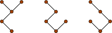
For instance, the number of binary trees having vertical profile $(2;2,1)$ is

\frac{2}{2\times 1}{3\choose 1}{1\choose 1}{1\choose 0}=3,

and these trees are shown in Figure 2.

Refer to caption — Figure 2. The three rooted binary trees having vertical profile $(2;2,1)$ .

This unexpected formula has first an obvious combinatorial interest: its proof – especially a bijective proof – has to shed a new light on the combinatorics of binary trees, which are of course eminently classical objects. But our original motivation lies in the link between the vertical profile of binary trees and a certain random probability measure, called the integrated superbrownian excursion, or ISE. The ISE is the limit, as $n$ increases, of the (normalized) occupation measure of a uniform random tree $T$ having $n$ vertices [29]. The normalized occupation measure of $T$ is defined to be

\mu_{n}=\frac{1}{n}\sum_{v\in T}\delta_{a(v)n^{-1/4}},

where $\delta_{x}$ is the Dirac measure at $x$ and $a(v)$ denotes the abscissa of the vertex $v$ . Note the double normalization, first by $1/n$ (to obtain a probability distribution) and then by $n^{-1/4}$ (which is known to be the correct scaling to obtain a non-trivial limit). Theorem 1 thus describes explicitly the law of $\mu_{n}$ : indeed, the probability that

\mu_{n}(i\,n^{-1/4})=\frac{n_{i}}{n}\quad\hbox{ for all }i\in\llbracket\ell,r\rrbracket

(and $\mu_{n}(in^{-1/4})=0$ for other values of $i$ ), with $n=\sum_{i}n_{i}$ , is the number of Theorem 1, divided by $C_{n}={2n\choose n}/(n+1)$ , the number of binary trees of size $n$ .

The ISE is not only related to binary trees. In fact, it appears to be a “universal” measure associated with numerous embedded branching structures [2, 16, 24, 27, 31, 33]. Due to the existence of bijections between certain families of rooted planar maps and embedded trees, it also describes (up to a translation) the limiting distribution of distances to the root vertex in planar maps of large size [8, 9, 13, 14, 34, 30]. Similar connections actually exist for maps on any orientable surface, for which the limiting distribution of distances is explicitly related to the ISE [11]. The law of the ISE is the subject of a very active research [6, 7, 15, 17, 12, 23, 27, 28], and we hope that knowing explicitly the law of $\mu_{n}$ will eventually yield a better understanding of the law of the ISE. For instance, the law of the support of the ISE, and the law of its density at one point, have already been determined though the study of embedded binary trees [6, 7].

Let us now return to Theorem 1. This theorem is not isolated: for instance, we prove a similar formula for embedded ternary trees. But our results also deal with embedded Cayley trees. Recall that a (rooted) Cayley tree of size $n$ is a tree (in the graph-theoretic sense) on the vertex set $V=\{1,2,\ldots,n\}$ , with a distinguished vertex $\rho$ called the root. An embedding of such a tree in ${\mathbb{Z}}$ is a map $a:V\rightarrow{\mathbb{Z}}$ such that $a(\rho)=0$ and $|a(v)-a(v^{\prime})|=1$ if $v$ and $v^{\prime}$ are neighbours. We call $a(v)$ the abscissa of $v$ . The vertical profile of this embedded tree is $(n_{\ell},\ldots,n_{-1};n_{0},n_{1},\ldots,n_{r})$ , where $n_{i}$ is the number of vertices at abscissa $i$ , and $\ell$ (resp. $r$ ) is the smallest (resp. largest) abscissa occurring in the tree. The counterpart of Theorem 1 for Cayley trees reads as follows.

Theorem 2.

Let $\ell\leq 0\leq r$ , and let $(n_{i})_{\ell\leq i\leq r}$ be a sequence of positive integers. The number of embedded rooted Cayley trees having vertical profile $(n_{\ell},\ldots,n_{-1};n_{0},n_{1},\ldots,n_{r})$ is

\frac{n_{0}}{n_{\ell}n_{r}}\frac{n!}{\prod\limits_{i=\ell}^{r}(n_{i}-1)!}\prod_{i=\ell}^{r}(n_{i-1}+n_{i+1})^{n_{i}-1},

where $n=\sum_{i}n_{i}$ is the number of vertices and $n_{\ell-1}=n_{r+1}=0$ .

For example, the number of Cayley trees having vertical profile $(2;2,1)$ is

\frac{2}{2\times 1}\frac{5!}{1!\times 1!\times 0!}\ 2^{1}\times 3^{1}\times 2^{0}=5!\times 6.

The shapes of these trees are shown in Figure 3. The positions of the vertices indicate their abscissas, but the labels of the nodes (in the interval $\llbracket 1,5\rrbracket$ ) are not indicated. To each of the first 5 shapes there corresponds $5!$ Cayley trees. To each of the last 2 shapes there corresponds $5!/2$ Cayley trees.

Theorems 1 and 2 can be proved using the multivariate Lagrange inversion formula, as will be shown in Section 7. Theorem 2 can also be proved using the matrix-tree theorem. However, non-trivial cancellations occur during the calculation, and the simple product forms remain mysterious. This is why we focus in the paper on bijective proofs, which explain directly the product forms. Moreover, these proofs allow us to consider other abscissa increments than $\pm 1$ (with the condition that the largest increment is 1). They also allow us to refine the enumeration, by taking into account the number of vertices at abscissa $j$ whose parent lies at abscissa $i$ , and/or the number of vertices at abscissa $i$ having a prescribed number of children at abscissa $j$ , for all $i$ and $j$ . In particular, we can impose that each vertex has at most one child of each abscissa, and the binary trees of Theorem 1 will in fact be seen (up to a symmetry factor of $n!$ , where $n$ is the number of vertices) as rooted Cayley trees such that each vertex of abscissa $i$ has at most one child at abscissa $i+1$ and at most one child at abscissa $i-1$ .

Our enumerative results are presented in the next section. We describe in Section 3 a first, basic bijection. It transforms certain functions into embedded trees, and is close to a bijection constructed by Joyal to count Cayley trees [25]. Section 4 collects simple enumerative results on functions, and converts them, via our bijection, into results on trees. Unfortunately, this basic bijection only proves the results of Section 2 for trees with non-negative labels. In Section 5, we design a much more involved variant of the basic bijection, which proves the remaining results (in Section 6). Finally, we discuss in Section 7 two other approaches to count embedded trees, namely functional equations coupled with the multivariate Lagrange inversion formula, and the matrix-tree theorem. These approaches require less invention, but they do not explain the product forms, and they prove only part of our results.

2. Main results

2.1. Embedded trees: definitions

A rooted Cayley tree of size $n$ is a tree (that is, an acyclic connected graph) on the vertex set $V=\{1,\ldots,n\}$ , with a distinguished vertex called the root.

Let $\mathcal{S}\subset{\mathbb{Z}}$ be a set of integers. An $\mathcal{S}$ -embedded Cayley tree is a rooted Cayley tree in which every vertex $v$ is assigned an abscissa $a(v)\in{\mathbb{Z}}$ in such a way:

•

the abscissa of the root vertex is $0$ ,
•

if $v^{\prime}$ is a child of $v$ , then $a(v^{\prime})-a(v)\in\mathcal{S}$ .

The vertical profile of the tree is $(n_{\ell},\ldots,n_{-1};n_{0},n_{1},\ldots,n_{r})$ , where $n_{i}$ is the number of nodes at abscissa $i$ , and $\ell$ (resp. $r$ ) is the smallest (resp. largest) abscissa found in the tree. The tree is non-negative if all vertices lie at a non-negative abscissa. Equivalently, $\ell=0$ .

Let $m=\min\mathcal{S}$ and $M=\max\mathcal{S}$ . The type of a vertex $v$ is $(i;s;c^{m},\ldots,c^{M})$ , where $i=a(v)$ is the abscissa of $v$ , $i-s$ is the abscissa of its parent (if $v$ is the root, we take $s=\varepsilon$ ), and for $m\leq k\leq M$ , $c^{k}$ is the number of children of $v$ at abscissa $i+k$ . Note that $s\in\mathcal{S}\cup\{\varepsilon\}$ . We often denote $\mbox{\boldmath$c$}:=(c^{m},\ldots,c^{M})\in{\mathbb{N}}^{M+1-m}$ . The out-type of $v$ is simply $(i;s)$ . Its in-type is $(i;\mbox{\boldmath$c$})$ . The reason for this terminology is that the edges are considered to be oriented towards the root. We sometimes call $(i;s;\mbox{\boldmath$c$})$ the complete type of $v$ .

An embedded Cayley tree is injective if two distinct vertices lying at the same abscissa have different parents. Equivalently, every vertex $v$ has at most one child at abscissa $a(v)+s$ , for all $s\in\mathcal{S}$ . Two embedded Cayley $T$ and $T^{\prime}$ trees are equivalent if they only differ by a renaming of the vertices. More precisely, if $T$ and $T^{\prime}$ have size $n$ , they are equivalent if there exists a bijection $f$ on $\llbracket 1,n\rrbracket$ that

•

respects the tree: if $w$ is the parent of $v$ in $T$ , then $f(w)$ is the parent of $f(v)$ in $T^{\prime}$ ,
•

respects abscissas: the abscissas of $v$ in $T$ and $f(v)$ in $T^{\prime}$ are the same.

An example in shown in Figure 4. Finally, an $\mathcal{S}$ -ary tree is an equivalence class of $\mathcal{S}$ -embedded injective Cayley trees. Thus an $\mathcal{S}$ -ary tree can be seen as an (unlabelled) rooted plane tree, drawn in the plane is such a way the root lies at abscissa 0, and each vertex $v$ has at most one child at abscissa $a(v)+s$ , for all $s\in\mathcal{S}$ . For instance, a $\{-1,1\}$ -ary tree is a binary tree that is canonically embedded, as shown in Figure 2. Similarly, a $\{-1,0,1\}$ -ary tree is a canonically embedded ternary tree [26]. Since injective trees have no symmetry, the $n!$ ways one can label the vertices of a given $\mathcal{S}$ -ary tree of size $n$ give rise to exactly $n!$ distinct injective $\mathcal{S}$ -embedded Cayley trees.

2.2. The vertical profile

Our first results deal with the number of embedded trees having a prescribed profile. As all results in this paper, they require the largest element of $\mathcal{S}$ to be 1. This condition is reminiscent of the enumeration of lattice paths in the half-line ${\mathbb{N}}$ , for which simple formulas exist provided the set $\mathcal{S}$ of allowed steps satisfies $\max\mathcal{S}=1$ ; see for instance [20, p. 75].

Theorem 3 (Embedded Cayley trees).

Let $\mathcal{S}\subset{\mathbb{Z}}$ such that $\max\mathcal{S}=1$ . Let $\ell\leq 0\leq r$ , and let $(n_{i})_{\ell\leq i\leq r}$ be a sequence of positive integers. If $\min\mathcal{S}=-1$ or $\ell=0$ , the number of $\mathcal{S}$ -embedded Cayley trees having vertical profile $(n_{\ell},\ldots,n_{-1};n_{0},n_{1},\ldots,n_{r})$ is

\frac{n_{0}}{n_{\ell}n_{r}}\frac{n!}{\prod\limits_{i=\ell}^{r}(n_{i}-1)!}\prod\limits_{i=\ell}^{r}\left(\sum_{s\in\mathcal{S}}n_{i-s}\right)^{n_{i}-1},

where $n=\sum_{i}n_{i}$ is the number of vertices and $n_{i}=0$ if $i<\ell$ or $i>r$ .

When $\mathcal{S}=\{-1,1\}$ , this theorem specializes to Theorem 2.

Remarks
1. This formula has several interesting specializations. When $0\in\mathcal{S}$ and $\ell=r=0$ , every vertex lies at abscissa $0$ and we are just counting rooted Cayley trees of size $n=n_{0}$ . Accordingly, the above formula is $n^{n-1}$ .

If $\mathcal{S}=\{1\}$ , each rooted Cayley tree has a unique $\mathcal{S}$ -embedding, and a vertex at distance $i$ from the root lies at abscissa $i$ . Hence the vertical profile of the tree coincides with its horizontal profile. The above theorem thus gives the number of rooted Cayley trees with horizontal profile $(1,n_{1},\ldots,n_{r})$ as

\frac{n!}{n_{1}!\cdots n_{r}!}\prod_{i=1}^{r-1}n_{i}^{n_{i+1}}

with $n=1+n_{1}+\cdots+n_{r}$ . This formula has a straightforward explanation: the multinomial coefficient describes the choice of the vertices lying at height $i$ , for all $i$ , and the factor $n_{i}^{n_{i+1}}$ describes how to choose a parent for each vertex lying at height $i+1$ .

If $\mathcal{S}=\{-1,1\}$ and $\ell=0$ , $r=1$ , the above theorem gives the number of bicolored Cayley trees, rooted at a white vertex, having $n_{0}$ white vertices and $n_{1}$ black vertices:

n_{0}{n_{0}+n_{1}\choose n_{0}}n_{1}^{n_{0}-1}n_{0}^{n_{1}-1}.

Equivalently, the number of spanning trees of the complete bipartite graph $K_{n_{0},n_{1}}$ is $n_{1}^{n_{0}-1}n_{0}^{n_{1}-1}$ (for references on this result, see the solution of Exercise 5.30 in [35]).

2. The assumption that the numbers $n_{i}$ are positive is not restrictive. Indeed, if $(n_{\ell},\ldots;n_{0},\ldots,n_{r})$ is the profile of an $\mathcal{S}$ -embedded tree, and the above conditions on $\mathcal{S}$ and $\ell$ hold, then $n_{\ell},\ldots,n_{r}$ are positive. Indeed, by definition of the profile, $n_{\ell}>0$ and $n_{r}>0$ . Moreover, the fact that the root lies at abscissa 0, and the condition $\max\mathcal{S}=1$ , imply that $n_{0},n_{1},\ldots,n_{r-1}$ are also positive. Finally, if $\ell<0$ , then we are assuming that $\min\mathcal{S}=-1$ , so that, symmetrically, $n_{\ell+1},\ldots,n_{-1}$ are positive.

3. It seems that no simple product formula exists¹¹ 1 See however the note at the end of this paper and the more recent paper [4] for a (less explicit) formula that applies more generally. when $\ell<0$ and $\min\mathcal{S}<-1$ . For instance, when $\mathcal{S}=\{-2,-1,1\}$ , the number of $\mathcal{S}$ -embedded trees with vertical profile $(1,1,1,2,1;1)$ is $6!\,\frac{3\cdot 107}{2}$ , and $107$ is prime (this number can be easily obtained from a recursive description of trees, as discussed in Section 7.1).

Symmetrically, if $\mathcal{S}=\{-1,1,2\}$ , there are $6!\,\frac{3\cdot 107}{2}$ $\mathcal{S}$ -embedded trees with vertical profile $(1,1,2,1,1,1)$ , which shows that the assumption $\max\mathcal{S}=1$ is also needed, even when $\ell=0$ .

4. It suffices to prove the theorem when $\ell=0$ . Indeed, assume $\ell<0$ and $\min\mathcal{S}=-1$ . We claim that the number of $\mathcal{S}$ -embedded trees having profile $(n_{\ell},\ldots;n_{0},\ldots,n_{r})$ and a marked vertex $v$ at abscissa $\ell$ equals the number of $\mathcal{S}$ -embedded trees with profile $(m_{0},\ldots,m_{r-\ell}):=(n_{\ell},\ldots,n_{0},\ldots,n_{r})$ (no semi-colon!) having a marked vertex at abscissa $-\ell$ . This follows from re-rooting the tree at $v$ (that is, choosing the vertex $v$ as the new root of the tree), marking the former root and then translating the abscissas by $-\ell$ . The resulting tree is a $\mathcal{S}$ -embedded tree because, when $\min\mathcal{S}=-1$ , the set of increments is symmetric. Thus, the number $T(n_{\ell},\ldots;n_{0},\ldots,n_{r})$ of trees having profile $(n_{\ell},\ldots;n_{0},\ldots,n_{r})$ satisfies

$\displaystyle n_{\ell}\,T(n_{\ell},\ldots;n_{0},\ldots,n_{r})$	$\displaystyle=$	$\displaystyle m_{-\ell}T(m_{0},\ldots,m_{r-\ell})$
	$\displaystyle=$	$\displaystyle\frac{m_{-\ell}}{m_{r-\ell}}\prod_{i=0}^{r-\ell}\left(\sum_{s\in\mathcal{S}}m_{i-s}\right)^{m_{i}-1}\hskip 5.69054pt(\hbox{case }\ell=0\hbox{ of Theorem~\ref{thm:cayley-profile}})$
	$\displaystyle=$	$\displaystyle\frac{n_{0}}{n_{r}}\prod_{i=\ell}^{r}\left(\sum_{s\in\mathcal{S}}n_{i-s}\right)^{n_{i}-1}\hskip 22.76219pt(\hbox{because }m_{i}=n_{i+\ell}),$

which gives the announced expression of $T(n_{\ell},\ldots;n_{0},\ldots,n_{r})$ .

Let us now state the counterpart of Theorem 3 for $\mathcal{S}$ -ary trees.

Theorem 4 ( $\mathcal{S}$ -ary trees).

Let $\mathcal{S}\subset{\mathbb{Z}}$ such that $\max\mathcal{S}=1$ . Let $\ell\leq 0\leq r$ , and let $(n_{i})_{\ell\leq i\leq r}$ be a sequence of positive integers. If $\min\mathcal{S}=-1$ or $\ell=0$ , the number of $\mathcal{S}$ -ary trees having vertical profile $(n_{\ell},\ldots,n_{-1};n_{0},n_{1},\ldots,n_{r})$ is

\frac{n_{0}}{n_{\ell}n_{r}}{\sum\limits_{s\in\mathcal{S}}n_{-s}\choose n_{0}-1}\prod_{\ell\leq i\leq r\atop i\not=0}{{\sum\limits_{s\in\mathcal{S}}n_{i-s}-1}\choose{n_{i}-1}},

with $n_{i}=0$ if $i<\ell$ or $i>r$ .

When $\mathcal{S}=\{-1,1\}$ , this theorem specializes to Theorem 1.

Remarks
1. It seems that no simple product formula exists²² 2 We refer again to the more recent paper [4] for a (less explicit) formula that applies more generally. when $\ell<0$ and $\min\mathcal{S}<-1$ . For instance, when $\mathcal{S}=\{-2,-1,1\}$ , the number of $\mathcal{S}$ -ary trees with vertical profile $(1,1,1,2,1;1)$ is $107$ , which is prime.

Symmetrically, if $\mathcal{S}=\{-1,1,2\}$ , there are $107$ $\mathcal{S}$ -ary trees with vertical profile $(1,1,2,1,1,1)$ , which shows that the assumption $\max\mathcal{S}=1$ is also needed, even when $\ell=0$ .

2. Rerooting an $\mathcal{S}$ -ary tree does not always give an $\mathcal{S}$ -ary tree, even if $\min\mathcal{S}=-1$ (think of re-rooting the first tree of Figure 2 at the lowest vertex of abscissa $-1$ ). Thus the case $\ell<0$ of Theorem 4 does not follow from the case $\ell=0$ , at least in an obvious way. It would be interesting to explore the combinatorial connection between these two cases.

2.3. The out-types

We now prescribe the number $n(i,s)$ of vertices of out-type $(i;s)$ , for all $i\in{\mathbb{Z}}$ and $s\in\mathcal{S}$ . In particular, the number $n_{i}$ of vertices at abscissa $i$ is determined, equal to ${\bf 1}_{i=0}+\sum_{s}n(i,s)$ . In other words, the profile is fixed.

Theorem 5 (Embedded Cayley trees).

Let $\mathcal{S}\subset{\mathbb{Z}}$ such that $\max\mathcal{S}=1$ . Let $n(i,s)$ be non-negative integers, for $i\in{\mathbb{Z}}$ and $s\in\mathcal{S}$ , and assume that either $\min\mathcal{S}=-1$ , or $n(i,s)=0$ for all $i<0$ and $s\in\mathcal{S}$ . The number of $\mathcal{S}$ -embedded Cayley trees in which, for all $i\in{\mathbb{Z}}$ and $s\in\mathcal{S}$ , exactly $n(i,s)$ non-root vertices have out-type $(i;s)$ is

\frac{n!\prod\limits_{i=\ell}^{r}n_{i}^{c(i)-1}\prod\limits_{i=\ell}^{-1}n(i,-1)\prod\limits_{i=1}^{r}n(i,1)}{\prod\limits_{i,s}n(i,s)!},

where $n$ is the number of vertices, $(n_{\ell},\ldots,n_{-1};n_{0},\ldots,n_{r})$ is the profile corresponding to the numbers $n(i,s)$ , and $c(i)$ is the number of vertices whose parent lies at abscissa $i$ :

n=\sum_{i}n_{i},\quad\quad n_{i}=\sum_{s}n(i,s)+{\bf 1}_{i=0},\quad\quad c(i)=\sum_{s}n(i+s,s).

When the range of a product or sum is not indicated, it is the ‘natural’ one ( $s\in\mathcal{S}$ , $i\in{\mathbb{Z}}$ ). It is assumed that $n_{i}>0$ for $\ell\leq i\leq r$ .

Remarks
1. An equivalent formulation consists in giving the generating function of $\mathcal{S}$ -embedded Cayley trees of vertical profile $(n_{\ell},\ldots;n_{0},\ldots,n_{r})$ , where a variable $x_{i,s}$ keeps track of the number of vertices of out-type $(i;s)$ . One easily checks that the above theorem boils down to saying that this generating function is

\frac{n_{0}}{n_{\ell}n_{r}}\frac{n!}{\prod\limits_{i=\ell}^{r}(n_{i}-1)!}\prod_{i=\ell}^{-1}x_{i,-1}\prod_{i=1}^{r}x_{i,1}\prod\limits_{i=\ell}^{r}\left(\sum_{s\in\mathcal{S}}n_{i-s}x_{i,s}\right)^{n_{i}-1}.

(2)

This formula refines of course Theorem 3, obtained by setting $x_{i,s}=1$ for all $i$ and $s$ .

2. As pointed out in [4], this theorem follows from [5, Eq. (23)], upon identifying the cofactor that occurs in that formula as a number of trees (which is simple to determine).

Let us now state the counterpart of Theorem 5 for $\mathcal{S}$ -ary trees.

Theorem 6 ( $\mathcal{S}$ -ary trees).

Let $\mathcal{S}\subset{\mathbb{Z}}$ such that $\max\mathcal{S}=1$ . Let $n(i,s)$ be non-negative integers, for $i\in{\mathbb{Z}}$ and $s\in\mathcal{S}$ , and assume that either $\min\mathcal{S}=-1$ , or $n(i,s)=0$ for all $i<0$ and $s\in\mathcal{S}$ . The number of $\mathcal{S}$ -ary trees in which, for all $i\in{\mathbb{Z}}$ and $s\in\mathcal{S}$ , exactly $n(i,s)$ non-root vertices have out-type $(i;s)$ is

\frac{\prod\limits_{i=\ell}^{-1}n(i,-1)\prod\limits_{i=1}^{r}n(i,1)}{\prod\limits_{i=\ell}^{r}n_{i}}\prod\limits_{i,s}{n_{i-s}\choose n(i,s)},

where $(n_{\ell},\ldots,n_{-1};n_{0},\ldots,n_{r})$ is the profile corresponding to the numbers $n(i,s)$ . Again, it is assumed that $n_{i}>0$ for $\ell\leq i\leq r$ .

Remark. It seems that no simple counterpart of (2) exists. That is, the generating function of $\mathcal{S}$ -ary trees of vertical profile $(n_{\ell},\ldots;n_{0},\ldots,n_{r})$ , taking into account the out-types of the vertices, does not factor nicely.

2.4. The in-types

We now prescribe the number $n(i,\mbox{\boldmath$c$})$ of vertices of in-type $(i;\mbox{\boldmath$c$})$ , for all $i$ and $\mbox{\boldmath$c$}=(c^{m},\ldots,c^{M})$ , with $m=\min\mathcal{S}$ and $M=\max\mathcal{S}$ . By definition of the in-types, it suffices to study the case where $\mathcal{S}=\llbracket m,M\rrbracket$ .

Note that the number $n_{i}$ of vertices at abscissa $i$ is determined, equal to $\sum_{\mbox{\scriptsize\boldmath$c$}}n(i,\mbox{\boldmath$c$})$ . Hence the profile $(n_{\ell},\ldots;n_{0},\ldots,n_{r})$ is fixed. The number $n(i,s)$ of vertices of out-type $(i;s)$ is also determined by the choice of the numbers $n(i,\mbox{\boldmath$c$})$ . Indeed, $n(i,s)$ is the number of edges going from a vertex of abscissa $i$ to its parent of abscissa $i-s$ , so that

n(i,s)=\sum_{\mbox{\scriptsize\boldmath$c$}}c^{s}n(i-s,\mbox{\boldmath$c$}).

Since we can express $n_{i}$ in terms of the numbers $n(i,s)$ or in terms of the numbers $n(i,\mbox{\boldmath$c$})$ , the following compatibility condition is required: for $\ell\leq i\leq r$ ,

{\bf 1}_{i=0}+\sum_{s,\mbox{\scriptsize\boldmath$c$}}c^{s}n(i-s,\mbox{\boldmath$c$})=\sum_{\mbox{\scriptsize\boldmath$c$}}n(i,\mbox{\boldmath$c$}).

We will also assume, as before, that $n_{\ell},\ldots,n_{r}$ are positive.

Theorem 7.

Let $m\leq 1$ and $\mathcal{S}=\llbracket m,1\rrbracket$ . Let $n(i,\mbox{\boldmath$c$})$ be non-negative integers, for $i\in{\mathbb{Z}}$ and $\mbox{\boldmath$c$}\in{\mathbb{N}}^{2-m}$ , satisfying the above compatibility condition. Assume moreover that either $m=-1$ , or $n(i,\mbox{\boldmath$c$})=0$ for all $i<0$ and $\mbox{\boldmath$c$}\in{\mathbb{N}}^{2-m}$ . The number of $\mathcal{S}$ -embedded Cayley trees in which, for all $i\in{\mathbb{Z}}$ and $\mbox{\boldmath$c$}\in{\mathbb{N}}^{2-m}$ , exactly $n(i,\mbox{\boldmath$c$})$ vertices have in-type $(i;\mbox{\boldmath$c$})$ is

\frac{n!\prod\limits_{i=\ell}^{r}(n_{i}-1)!}{\prod\limits_{i,\mbox{\scriptsize\boldmath$c$}}n(i,\mbox{\boldmath$c$})!\prod\limits_{b\geq 0,s}b!^{n_{s}(b)}}\prod\limits_{i=\ell}^{-1}n(i,-1)\prod\limits_{i=1}^{r}n(i,1),

where $n$ is the number of vertices, $(n_{\ell},\ldots,n_{-1};n_{0},\ldots,n_{r})$ is the profile corresponding to the numbers $n(i,\mbox{\boldmath$c$})$ , $n_{s}(b)$ is the number of vertices $v$ that have exactly $b$ children at abscissa $a(v)+s$ , and $n(i,s)$ is the number of vertices of out-type $(i,s)$ . Equivalently,

\displaystyle n=\sum_{i}n_{i},\quad\quad n_{i}=\sum_{\mbox{\scriptsize\boldmath$c$}}n(i,\mbox{\boldmath$c$}),\quad\quad n_{s}(b)=\sum_{i}\sum_{\mbox{\scriptsize\boldmath$c$}:c^{s}=b}n(i,\mbox{\boldmath$c$}),\quad\quad n(i,s)=\sum_{\mbox{\scriptsize\boldmath$c$}}c^{s}n(i-s,\mbox{\boldmath$c$}).

Remarks
1. Again, this theorem has interesting specilizations. Assume for instance that $n(i,\mbox{\boldmath$c$})=0$ as soon as $i\not=0$ , and $m=0$ . Then the only non-zero numbers $n(i,\mbox{\boldmath$c$})$ are of the form $n(0,i,0):=k_{i}$ , giving the number of vertices of the tree having $i$ children. In particular, $n_{0}=n$ . The above formula reads

\frac{n!(n-1)!}{\prod_{i}k_{i}!\prod_{i}i!^{k_{i}}},

and gives the number of rooted Cayley trees having $k_{i}$ vertices of in-degree $i$ [35, Corollary 5.3.5].

If $\mathcal{S}=\{1\}$ , each rooted Cayley tree has a unique $\mathcal{S}$ -embedding, and a vertex at distance $i$ from the root lies at abscissa $i$ . The above theorem gives the number of rooted Cayley trees in which $k(i,c)$ vertices have height $i$ and (in-)degree $c$ , for all $i$ and $c$ :

\frac{n!}{\prod_{i,c}k(i,c)!}\prod_{i=1}^{r}\frac{n_{i}!}{\prod_{c}c!^{k(i-1,c)}}.

This formula has a direct explanation: the multinomial coefficient describes the choice of the vertices of indegree $c$ lying at height $i$ , for all $i$ and $c$ and the multinomial $\frac{n_{i}!}{\prod_{c}c!^{k(i-1,c)}}$ how to assign children to vertices of height $i-1$ .

If $\mathcal{S}=\{-1,1\}$ and $\ell=0$ , $r=1$ , the above theorem gives the number of bicolored Cayley trees, rooted at a white vertex, having $k(0,c)$ white vertices of (in-)degree $c$ and $k(1,c)$ black vertices of (in-)degree $c$ for all $c$ :

\frac{(n_{0}+n_{1})!(n_{0}-1)!n_{1}!}{\prod_{i,c}k(i,c)!\prod_{c}c!^{k(0,c)+k(1,c)}},

(3)

with $n_{i}=\sum_{c}k(i,c)$ . This is related to a known formula that gives the number of spanning trees of the complete bipartite graph $K_{m_{0},m_{1}}$ (with white vertices labelled $u_{1},\ldots,u_{m_{0}}$ and black vertices labelled $v_{1},\ldots,v_{m_{1}}$ ) in which each vertex has a prescribed degree:

\frac{(m_{0}-1)!(m_{1}-1)!}{\prod_{c}!^{k(0,c)+k(1,c)}},

(4)

where $k(0,c)$ (resp. $k(1,c)$ ) is the number of white (resp. black) vertices of total degree $c+1$ (see [35, Exercise 5.30] and [3]). Indeed, (3) can be derived from (4), taken with $m_{0}=n_{0}$ and $m_{1}=1+n_{1}$ , when $v_{1}$ has degree 1. Conversely, our results actually allow us to prescribe the in-type of the root and the number of white and black vertices of fixed in-type (see Section 4.5), and this refined formula implies (4).

2. If $n(i,\mbox{\boldmath$c$})=0$ as soon as one of the components of $c$ is larger than 1, then the trees counted by the above formula are injective. Thus it suffices to divide this formula by $n!$ to obtain the number of $\mathcal{S}$ -ary trees having $n(i,\mbox{\boldmath$c$})$ vertices of in-type $(i;\mbox{\boldmath$c$})$ for all $i$ and $c$ .

2.5. The complete types

We finally prescribe the in-type $(0;\mbox{\boldmath$c$}_{0})$ of the root and the number $n(i,s,\mbox{\boldmath$c$})$ of (non-root) vertices of (complete) type $(i;s;\mbox{\boldmath$c$})$ , for all $i$ , $s$ and $c$ . In particular, the number of vertices of out-type $(i,s)$ is fixed, and can be expressed in terms of the numbers $n(i,s,\mbox{\boldmath$c$})$ in two different ways. This yields the following compatibility condition, for all $i$ and $s$ :

{\bf 1}_{i=s}c_{0}^{s}+\sum_{t,\mbox{\scriptsize\boldmath$c$}}c^{s}n(i-s,t,\mbox{\boldmath$c$})=\sum_{\mbox{\scriptsize\boldmath$c$}}n(i,s,\mbox{\boldmath$c$}).

We also assume, as before, that $n_{\ell},\ldots,n_{r}$ are positive.

We have only obtained a formula when $\ell=0$ and $0\not\in\mathcal{S}$ (plus the usual condition $\max\mathcal{S}=1$ ). We thus focus on the case $\mathcal{S}=\llbracket m,-1\rrbracket\cup\{1\}$ .

Theorem 8.

Let $m\leq 1$ and $\mathcal{S}=\llbracket m,-1\rrbracket\cup\{1\}$ . Let $\mbox{\boldmath$c$}_{0}=(0,\ldots,0,c_{0}^{1})\in{\mathbb{N}}^{2-m}$ . Let $n(i,s,\mbox{\boldmath$c$})$ be non-negative integers, for $i\in{\mathbb{Z}}$ , $s\in\mathcal{S}$ and $\mbox{\boldmath$c$}\in{\mathbb{N}}^{2-m}$ , such that $n(i,s,\mbox{\boldmath$c$})=0$ if $i<0$ or $c^{0}>0$ . Assume that the above compatibility condition holds. The number of $\mathcal{S}$ -embedded Cayley trees in which the root has in-type $(0;\mbox{\boldmath$c$}_{0})$ and for all $i\in{\mathbb{Z}}$ , $s\in\mathcal{S}$ and $\mbox{\boldmath$c$}\in{\mathbb{N}}^{2-m}$ , exactly $n(i,s,\mbox{\boldmath$c$})$ non-root vertices have type $(i;s;\mbox{\boldmath$c$})$ is

\frac{c_{0}^{1}\,n!\prod\limits_{i,s}n(i,s)!}{\prod\limits_{i,s,\mbox{\scriptsize\boldmath$c$}}n(i,s,\mbox{\boldmath$c$})!\prod\limits_{i=1}^{r}n(i,1)\prod\limits_{b\geq 0,s}b!^{n_{s}(b)}}\prod\limits_{i=1}^{r-1}\left(\sum\limits_{b>0}b\,n_{1}(i,1,b)\right),

where $n$ is the number of vertices, $r$ is the maximal abscissa, $n(i,s)$ is the number of vertices of out-type $(i;s)$ , $n_{s}(b)$ is the number of vertices $v$ that have exactly $b$ children at abscissa $a(v)+s$ , and $n_{1}(i,1,b)$ is the number of vertices of out-type $(i;1)$ that have exactly $b$ children at abscissa $i+1$ . That is,

\displaystyle n(i,s)=\sum_{\mbox{\scriptsize\boldmath$c$}}n(i,s,\mbox{\boldmath$c$}),\quad\quad n_{s}(b)=\sum_{i,t}\sum_{\mbox{\scriptsize\boldmath$c$}:c^{s}=b}n(i,t,\mbox{\boldmath$c$})+{\bf 1}_{s=1,b=c_{0}^{1}},\quad\quad n_{1}(i,1,b)=\sum_{\mbox{\scriptsize\boldmath$c$}:c^{1}=b}n(i,1,\mbox{\boldmath$c$}).

3. A bijection for non-negative trees

Let $n_{0},\ldots,n_{r}$ be a sequence of positive integers. Let $V=\cup_{i=0}^{r}V_{i}$ with $V_{i}=\{i^{1},\ldots,i^{n_{i}}\}$ . The elements of $V$ are called vertices, and the vertices of $V_{i}$ are said to have abscissa $i$ . The abscissa of a vertex $v$ is denoted by $a(v)$ . The vertices are totally ordered as follows:

i^{k}\leq j^{p}\Longleftrightarrow(i<j)\hbox{ or }(i=j\hbox{ and }k\leq p).

We consider partial functions $f$ on $V$ , which we regard as digraphs on the vertex set $V$ : for each vertex $v$ such that $f(v)$ is defined, an arc joins $v$ to $f(v)$ .

Let $\mathcal{S}\subset{\mathbb{Z}}$ with $\min\mathcal{S}=m$ and $\max\mathcal{S}=1$ . A partial function $f$ on $V$ is an $\mathcal{S}$ -function if for all $v=i^{k}$ such that $f(v)$ is defined,

f(i^{k})\in\cup_{s\in\mathcal{S}}V_{i-s}.

The type (or: complete type) of the vertex $v$ is $(i;s;c^{m},\ldots,c^{1})$ , where $i$ is the abscissa of $v$ , $i-s$ is the abscissa of $f(v)$ (or $\varepsilon$ if $f(v)$ is not defined), and for $m\leq k\leq 1$ , $c^{k}$ is the number of pre-images of $v$ at abscissa $i+k$ . We often denote $\mbox{\boldmath$c$}=(c^{m},\ldots,c^{1})$ . The out-type of $v$ is $(i;s)$ . Its in-type is $(i;\mbox{\boldmath$c$})$ . In the function shown in Figure 5, which is an $\mathcal{S}$ -function for $\mathcal{S}=\llbracket-2,1\rrbracket$ , the vertex $0^{1}$ has type $(0;\varepsilon;0,0,0,1)$ , and the vertex $2^{1}$ has type $(2;1;1,0,0,1)$ . An edge of a digraph is an $\mathcal{S}$ -edge if it joins a vertex of abscissa $i$ to a vertex of abscissa $i-s$ , for $s\in\mathcal{S}$ .

Figure 5. A

\{-2,-1,0,1\}

-function on

V=\{0^{1},\ldots,0^{5},1^{1},\ldots,1^{4},2^{1},\ldots,2^{10},3^{1},\ldots,3^{6}\}

Consider now a rooted tree $T$ on the vertex set $V$ . We say that $T$ is an $\mathcal{S}$ -tree if the parent of any (non-root) vertex of $V_{i}$ belongs to $\cup_{s\in\mathcal{S}}V_{i-s}$ . We orient the edges of $T$ towards the root: then $V$ can be seen as an $\mathcal{S}$ -function. This allows us to define the type, in-type and out-type of a vertex. A marked $\mathcal{S}$ -tree is a pair $(T,r^{q})$ consisting of an $\mathcal{S}$ -tree and a marked vertex $r^{q}\in V_{r}$ . There is a simple connection between $\mathcal{S}$ -trees and $\mathcal{S}$ -embedded Cayley trees, which will be made explicit in the next section. We focus for the moment on $\mathcal{S}$ -trees.

Theorem 9.

Let $n_{0},\ldots,n_{r}$ , $V$ and $\mathcal{S}$ be as above. There exists a bijection $\Phi$ between $\mathcal{S}$ -functions $f:V\setminus\{0^{1}\}\rightarrow V$ satisfying

(F)

for $1\leq i\leq r$ , $f(i^{1})=(i-1)^{1}$ ,

and marked $\mathcal{S}$ -trees $(T,r^{q})$ on the vertex set $V$ , rooted at the vertex $0^{1}$ and satisfying

(T)

on the path going from $r^{q}$ to $0^{1}$ , the first vertex belonging to $V_{i-1}$ is preceded by $i^{1}$ , for all $i\in\llbracket 1,r\rrbracket$ .

(The condition $\max\mathcal{S}=1$ implies that this path contains a vertex of $V_{i-1}$ for all $i$ .)

Moreover, the bijection $\Phi$

(a)

preserves the out-type of every vertex;
(b)

preserves the number of vertices of in-type $(i;\mbox{\boldmath$c$})$ , for all $i$ and $c$ ;

Proof.

The bijection $\Phi$ is the composition of two bijections $\Phi_{1}$ and $\Phi_{2}$ . The first bijection, $\Phi_{1}$ , transforms an $\mathcal{S}$ -function into an $\mathcal{S}$ -tree. It is a simple adaptation of a construction designed by Joyal to count Cayley trees [25, p. 16]. It satisfies Properties (a) and (c). However, if $0\in\mathcal{S}$ , it does not satisfy (b). The second bijection, $\Phi_{2}$ , remedies this problem by performing a simple re-arrangement of subtrees. If $0\not\in\mathcal{S}$ , then $\Phi_{2}$ is the identity, so that $\Phi=\Phi_{1}$ .

Figure 6. The map

\Phi_{1}

applied to the function of Figure 5. The marked vertex is

3^{4}

$\bullet$ The map $\Phi_{1}$ : from functions to trees
Let us describe the construction $\Phi_{1}$ . It is illustrated in Figure 6, where we construct the tree associated with the function of Figure 5 (which satisfies indeed Condition (F)).

Let $f:V\setminus\{0^{1}\}\rightarrow V$ be a function satisfying (F), and consider the associated digraph $G_{f}$ . One of its connected components contains the path $r^{1}\rightarrow(r-1)^{1}\rightarrow\cdots\rightarrow 1^{1}\rightarrow 0^{1}$ . Split each of the $r$ edges of this path into two half-edges (one in-going, one out-going), thus forming $r+1$ pieces. Each piece is of the form

We say that $i^{1}$ (or $r^{1}$ , or $0^{1}$ ) is the source (and also the sink) of this piece.

Each of the other components of $G_{f}$ contains exactly one cycle. In each of them, split into two half-edges the edge that goes into the smallest vertex, say $i^{k}$ , of the cycle. The vertices that formed the cycle now form a distinguished path in the resulting piece, starting from $i^{k}$ . Trees are attached to the vertices of this path, as shown below:

We say that $i^{k}$ is the source of this piece. The endpoint of the distinguished path is the sink of the piece. We say that the piece has type $(i,j$ ).

Lemma 10.

If $i^{k}$ and $j^{p}$ are respectively the source and the sink of a piece and $k\not=1$ , then $j=i+1$ , or $j=i$ with $p\geq k$ . The latter case only occurs if $0\in\mathcal{S}$ .

Proof.

We have $j^{p}\geq i^{k}$ (since $i^{k}$ was minimal in its cycle). Given that $f(j^{p})=i^{k}$ , and $\max\mathcal{S}=1$ , this means that either $j=i+1$ , or $j=i$ with $p\geq k$ .

Figure 7. A typical path from

r^{q}

0^{1}

, after concatenation of the pieces. It is assumed that

q>p_{1}

n_{3}>n_{2}>n_{1}

and

m_{3}>m_{2}>m_{1}

. The boxes show the distinguished paths of the pieces. The edges that join the boxes were not in the graph of the function

f

, unless they are of the form

(i+1)^{1}\rightarrow i^{1}

. The dashed edges that are not of the form

(i+1)^{1}\rightarrow i^{1}

were in the graph of

f

, but are not in the final tree.

Now, order the pieces from left to right by decreasing source: the first (leftmost) piece has source $r^{q}$ , for some $q\in\{1,\ldots,n_{r}\}$ , and the last (rightmost) piece has source $0^{1}$ . Concatenate them to form a single path going from $r^{q}$ to $0^{1}$ , keeping in place the attached trees. Note that there is a piece of source $i^{1}$ , for all $i\in\llbracket 0,r\rrbracket$ . A typical path from $r^{q}$ to $0^{1}$ is shown in Figure 7. The resulting graph is a tree rooted at $0^{1}$ . In this tree, we mark the vertex $r^{q}$ . We define this marked tree to be $\Phi_{1}(f)$ .

Proposition 11.

The map $\Phi_{1}$ satisfies all properties stated in Theorem 9, apart from (b).

Proof.

Let us first prove that $\Phi_{1}$ is injective. Observe that the sources of the pieces are the lower records met on the path from $r^{q}$ to $0^{1}$ . This allows us to recover the collection of pieces by splitting into two half-edges each edge of this path that goes into a lower record. From the pieces, it is easy to reconstruct the function $f$ : one adds an edge from $i^{1}$ to $(i-1)^{1}$ for $i\in\llbracket 1,r\rrbracket$ , and then connects the two extremal half-edges in each remaining piece to form a cycle. Thus $\Phi_{1}$ is injective.

It is clear from the construction (and its illustration in Figure 7) that the out-types are preserved. In particular, $\Phi_{1}(f)$ is an $\mathcal{S}$ -tree. It satisfies (T) by construction. Note that the in-type of vertices may change. However, this only happens for source vertices. In the example of Figure 6, the in-type of each source other than $1^{1}$ has changed.

Let us now prove (c). Assume $0\not\in\mathcal{S}$ . By Lemma 10, a piece of source $i^{k}$ and sink $j^{p}$ satisfies $j=i+1$ , provided $k>1$ . Thus the path going from $r^{q}$ to $0^{1}$ in $\Phi_{1}(f)$ has a simpler form:

In particular, the marked vertex is $r^{1}$ . It is now easy to check that each vertex has the same type in $\Phi_{1}(f)$ as in $f$ , so that (c) holds.

It remains to prove that $\Phi_{1}$ is surjective. Take a marked $\mathcal{S}$ -tree $(T,r^{q})$ , rooted at $0^{1}$ and satisfying (T). Let us call the path going from $r^{q}$ to $0^{1}$ the distinguished path of $T$ . Each lower record of this path is called a source. Each vertex that precedes a source (plus the vertex $0^{1}$ ) is called a sink. In the distinguished path, split into two half-edges each edge that goes into a source. This gives a number of pieces, formed of a distinguished path starting at a source and ending at a sink, to which trees are attached. By Condition (T), each vertex $i^{1}$ is a lower record, followed (when $i>0$ ) by another one. Thus there is a piece of source and sink $i^{1}$ , for all $i\in\llbracket 0,r\rrbracket$ . Concatenate the pieces of source $i^{1}$ to form a path $r^{1}\rightarrow\cdots\rightarrow 0^{1}$ . In each of the other pieces, close the distinguished path to form a cycle. The resulting graph $G$ is the graph of a function $g:V\setminus\{0^{1}\}\rightarrow V$ . It satisfies (F) by construction. As observed when proving injectivity, if $(T,r^{q})=\Phi_{1}(f)$ , where $f$ is an $\mathcal{S}$ -function satisfying (F), then $f$ and $g$ coincide.

We claim that $g$ is always an $\mathcal{S}$ -function. We only need to check that each edge of $G$ that was not in the tree is an $\mathcal{S}$ -edge. Since $1\in\mathcal{S}$ , the edges $r^{1}\rightarrow\cdots\rightarrow 0^{1}$ are $\mathcal{S}$ -edges. Now consider a piece of source $i^{k}$ , with $k>1$ . Its sink $j^{p}$ is followed in $T$ by a lower record that has also abscissa $i$ (because one of the lower records is $i^{1}$ ), say $i^{m}$ . The edge we add to form a cycle is $j^{p}\rightarrow i^{k}$ , and it is an $\mathcal{S}$ -edge since the edge $j^{p}\rightarrow i^{m}$ was an $\mathcal{S}$ -edge of $T$ .

Proposition 11 says that $\Phi_{1}$ fulfills almost all requirements of Theorem 9, apart from Condition (b). More specifically, the in-types of sources may change, and this only happens if $0\in\mathcal{S}$ . Our second transformation, $\Phi_{2}$ , performs on the tree $(T,r^{q}):=\Phi_{1}(f)$ a little surgery that remedies this problem.

$\bullet$ The map $\Phi_{2}$ : rearranging subtrees
Let $(T,r^{q})$ be a marked tree satisfying the conditions of Theorem 9. Let $f=\Phi_{1}^{-1}(T,r^{q})$ . Consider the section of the distinguished path of $T$ comprised between the vertices $(i+1)^{1}$ and $i^{1}$ (we assume for the moment that $i<r$ ). The first piece of this section has source and sink $(i+1)^{1}$ , while all other pieces, including the final one with source $i^{1}$ , have type $(i,i)$ or $(i,i+1)$ :

We say that a source $v$ of abscissa $i$ is frustrated if its in-type is not the same in $T$ and $f$ . The above figure, in which frustrated sources are indicated with an exclamation mark, shows that this happens in two cases.

Observation 12.

A source $v$ of abscissa $i<r$ is frustrated if and only if one of the following conditions holds:

•

the sink of the piece containing $v$ has abscissa $i$ , but the sink of piece that precedes $v$ has abscissa $i+1$ ,
•

the sink of the piece containing $v$ has abscissa $i+1$ , but the sink of piece that precedes $v$ has abscissa $i$ .

In the former (resp. latter) case, we say that $v$ is $i$ -frustrated (resp. $(i+1)$ -frustrated). The key observation that will allow us to preserve in-types after a small surgery is the following.

Observation 13.

Consider the frustrated vertices of abscissa $i$ met on the distinguished path of $T$ . Then $i$ -frustrated vertices and $(i+1)$ -frustrated vertices alternate, starting with an $i$ -frustrated vertex, and ending with an $(i+1)$ -frustrated vertex.

Recall that the marked tree $(T,r^{q})$ consists of subtrees attached to a distinguished path. If there are $2m$ frustrated vertices of abscissa $i$ , say $i^{k_{1}},\ldots,i^{k_{2m}}$ , to which the subtrees $\tau_{1},\ldots,\tau_{2m}$ are attached, exchange the subtrees $\tau_{2p-1}$ and $\tau_{2p}$ for all $p\in\llbracket 1,m\rrbracket$ (leaving their roots $i^{k_{1}},\ldots,i^{k_{2m}}$ in place). In the resulting tree, $i^{k_{2p-1}}$ inherits the in-type that $i^{k_{2p}}$ has in the function $f$ , and vice-versa. The in-type of non-frustrated vertices has not changed.

The surgery is simpler for frustrated vertices of abscissa $r$ , because there are no pieces of type $(r,r+1)$ .

Observation 14.

If the marked vertex is $r^{q}=r^{1}$ , there are no frustrated vertices at abscissa $r$ . Otherwise, the only two frustrated vertices at abscissa $r$ are $r^{1}$ and the marked vertex $r^{q}$ .

In the latter case we simply exchange the subtrees attached to $r^{1}$ and $r^{q}$ , so that $r^{q}$ inherits the in-type that $r^{1}$ has in $f$ , and vice-versa.

We define $\Phi_{2}(T,r^{q})$ to be the marked tree obtained after rearranging the subtrees of $(T,r^{q})$ , and $\Phi:=\Phi_{2}\circ\Phi_{1}$ . An example is shown in Figure 8, where we rearrange the subtrees of the tree $(T,r^{q})=\Phi_{1}(f)$ shown in Figure 6.

Figure 8. The map

\Phi_{2}

applied to the tree

(T,r^{q})

of Figure 6 (with

r^{q}=3^{4}

). The frustrated vertices are the same in

(T,r^{q})

and

\Phi_{2}(T)

, and are indicated by “!”.

We claim that $\Phi$ satisfies Theorem 9. Of course, the proof of this fact uses the properties of $\Phi_{1}$ stated in Proposition 11.

First, observe that the out-types are the same in $T$ and $\Phi_{2}(T,r^{q})$ (because vertices pointing to a frustrated source of abscissa $i$ in $T$ also point to a source of abscissa $i$ in $\Phi_{2}(T,r^{q})$ ). Hence $\Phi$ satisfies (a). It also satisfies (c), because there are no frustrated vertices if $0\not\in\mathcal{S}$ , so that $\Phi_{2}$ leaves all trees unchanged. Finally, the surgery performed by $\Phi_{2}$ is precisely designed to “correct” the in-types of frustrated vertices, while leaving unchanged the in-types of non-frustrated vertices. Hence $\Phi$ satisfies (b).

It remains to prove that $\Phi_{2}$ is bijective. A stronger property actually holds: $\Phi_{2}$ is an involution. Indeed, the distinguished paths of $(T,r^{q})$ and $\Phi_{2}(T,r^{q})$ coincide, and Observations 12 and 14 imply that the frustrated vertices of $(T,r^{q})$ and $\Phi_{2}(T,r^{q})$ are the same. Applying $\Phi_{2}$ to $\Phi_{2}(T,r^{q})$ just restores the marked tree $(T,r^{q})$ .

4. Enumeration of non-negative embedded trees

In this section, we prove the enumerative results of Section 2 in the case $\ell=0$ , that is, for non-negative trees. These results follow from the bijection of Theorem 9, combined with the enumeration of $\mathcal{S}$ -functions (which, as we shall see, is an elementary exercise). We also need to relate the $\mathcal{S}$ -trees occurring in Theorem 9 to the $\mathcal{S}$ -embedded Cayley trees of Section 2. This is done in the following lemma. We adopt the same notation as in the previous section: $V=\cup_{i=0}^{r}V_{i}$ with $V_{i}=\{i^{1},\ldots,i^{n_{i}}\}$ , and $\mathcal{S}\subset{\mathbb{Z}}$ satisfies $\min\mathcal{S}=m$ and $\max\mathcal{S}=1$ . The type distribution of a tree is the collection of numbers $n(i,s,\mbox{\boldmath$c$})$ (with $i\in\llbracket 0,r\rrbracket$ , $s\in\mathcal{S}$ and $\mbox{\boldmath$c$}\in{\mathbb{N}}^{-m+2}$ ) giving the number of vertices of type $(i;s;\mbox{\boldmath$c$})$ .

Lemma 15.

The number of non-negative $\mathcal{S}$ -embedded Cayley trees having a prescribed type distribution is

\frac{1}{n_{r}}\frac{n!}{\prod_{i=0}^{r}(n_{i}-1)!}

times the number of marked $\mathcal{S}$ -trees satisfying Condition $(\rm T)$ of Theorem 9 and having the same type distribution (as always, $(n_{0},\ldots,n_{r})$ denotes the profile of the tree, and $n$ its size).

Proof.

Equivalently, we want to prove that the number of non-negative $\mathcal{S}$ -embedded Cayley trees having a prescribed type distribution and a marked vertex at abscissa $r$ is

\frac{n!}{\prod_{i}(n_{i}-1)!}

times the number of marked $\mathcal{S}$ -trees satisfying (T) and having the same type distribution. We will construct a 1-to- $n!/\prod_{i}(n_{i}-1)!$ correspondence between marked $\mathcal{S}$ -trees satisfying (T) and marked $\mathcal{S}$ -embedded Cayley trees, preserving the type distribution.

Let $(T,r^{q})$ be a marked $\mathcal{S}$ -tree on $V$ satisfying (T). On the path going from $r^{q}$ to $0^{1}$ , the first vertex of $V_{i-1}$ is preceded by $i^{1}$ , for $1\leq i\leq r$ . Let us rename the vertex $i^{1}$ by $i^{k}$ , for a $k$ chosen in $\{1,\ldots,n_{i}\}$ ; conversely, let us rename $i^{k}$ by $i^{1}$ . Let us also exchange the names of the vertices $0^{1}$ and $0^{p}$ , for a $p$ chosen in $\{1,\ldots,n_{0}\}$ . This gives an arbitrary $\mathcal{S}$ -tree $T_{1}$ , rooted at $0^{p}$ , with a marked vertex at abscissa $r$ . This tree may or may not satisfy (T). The number of different trees $T_{1}$ that can be constructed from $T$ in such a way is $\prod_{i=0}^{r}n_{i}$ . The marked tree $(T,r^{q})$ can be recovered from $(T_{1},r^{q})$ by restoring vertex names, since we know that $T$ is rooted at $0^{1}$ and satisfies (T).

Let us now assign labels from $\{1,\ldots,n\}$ , with $n=\sum_{i}n_{i}$ , to the vertices of $T_{1}$ , in such a way that the labels $a$ and $b$ assigned to $i^{k}$ and $i^{p}$ satisfy $a<b$ if $k<p$ . There are $n!/\prod_{i}n_{i}!$ ways to do so. Finally, erase all names $i^{k}$ from the tree, for all $i$ and $k$ . This gives an arbitrary rooted $\mathcal{S}$ -embedded Cayley tree $T_{2}$ , with a marked vertex at abscissa $r$ . The tree $T_{1}$ can be recovered from $T_{2}$ by renaming the vertices of abscissa $i$ with $i^{1},\ldots,i^{n_{i}}$ in the unique way that is consistent with the order on labels: if two vertices of labels $a$ and $b$ , with $a<b$ , lie at abscissa $i$ , then their names $i^{k}$ and $i^{p}$ must satisfy $k<p$ .

The marked $\mathcal{S}$ -tree $T$ has given rise to $n!/\prod_{i}(n_{i}-1)!$ marked embedded trees $T_{2}$ . Moreover, $T_{2}$ , $T_{1}$ and $T$ have the same type distribution. The result follows.

In what follows, we will count trees by counting functions, using the correspondence of Theorem 9. We will sometimes prescribe the type (or in-type, or out-type) of every vertex of $V$ , or just the number of vertices of each type (or in-type, or out-type). We will always assume that these type distributions are compatible with the conditions required for the function (by writing “assuming compatibility…”). For instance,

•
if we fix the type $(i_{v};s_{v};\mbox{\boldmath$c$}_{v})$ of each vertex $v\in V$ (or just the in-type or out-type), we assume that
- –
  
  $i_{v}=i$ if $v\in V_{i}$ ,
- –
  
  $s_{v}\in\mathcal{S}$ and $i_{v}-s_{v}\in\llbracket 0,r\rrbracket$ ,
- –
  
  $s_{v}=1$ if $v=i^{1}$ with $i>0$ , and $s_{v}=\varepsilon$ if $v=0^{1}$ ,
•

if the number $n(i,s)$ of vertices of $V$ of out-type $(i;s)$ , for all $i\in\llbracket 0,r\rrbracket$ and $s\in\mathcal{S}$ , is prescribed, we assume that $n(i,s)=0$ if $i-s\not\in\llbracket 0,r\rrbracket$ , and that

$n_{i}=\sum_{s}n(i,s)+{\bf 1}_{i=0},$

•

if the number $n(i,\mbox{\boldmath$c$})$ of vertices of $V$ of in-type $(i;\mbox{\boldmath$c$})$ , for all $i\in\llbracket 0,r\rrbracket$ and $\mbox{\boldmath$c$}\in{\mathbb{N}}^{2-m}$ is fixed (whether we prescribe it directly, or whether we prescribe the in-type of each vertex), we assume that $n(i,\mbox{\boldmath$c$})=0$ if $c^{s}>0$ for some $s\not\in\mathcal{S}$ , that

n_{i}=\sum_{\mbox{\scriptsize\boldmath$c$}}n(i,\mbox{\boldmath$c$}),

and also that the following condition, obtained by counting in two different ways the vertices of $V_{i}$ , holds:

{\bf 1}_{i=0}+\sum_{s,\mbox{\scriptsize\boldmath$c$}}c^{s}n(i-s,\mbox{\boldmath$c$})=\sum_{\mbox{\scriptsize\boldmath$c$}}n(i,\mbox{\boldmath$c$}),

•

finally, if we fix the out-type $\mbox{\boldmath$c$}_{0}$ of the vertex $0^{1}$ , and if the number $n(i,s,\mbox{\boldmath$c$})$ of vertices of $V$ of type $(i;s;\mbox{\boldmath$c$})$ , for all $i\in\llbracket 0,r\rrbracket$ , $s\in\mathcal{S}$ and $\mbox{\boldmath$c$}\in{\mathbb{N}}^{2-m}$ , is also fixed (whether we prescribe it directly, or whether we prescribe the type of each vertex), we assume that $n(i,t,\mbox{\boldmath$c$})=0$ if $c^{s}>0$ for some $s\not\in\mathcal{S}$ , that

n_{i}=\sum_{s,\mbox{\scriptsize\boldmath$c$}}n(i,s,\mbox{\boldmath$c$}),

and also that the following condition, obtained by counting in two different ways the vertices of out-type $(i,s)$ , holds:

{\bf 1}_{i=s}c_{0}^{s}+\sum_{t,\mbox{\scriptsize\boldmath$c$}}c^{s}n(i-s,t,\mbox{\boldmath$c$})=\sum_{\mbox{\scriptsize\boldmath$c$}}n(i,s,\mbox{\boldmath$c$}).

4.1. The profile of $\mathcal{S}$ -embedded Cayley trees: proof of Theorem 3

By Lemma 15, the number of $\mathcal{S}$ -embedded Cayley trees having vertical profile $(n_{0},\ldots,n_{r})$ is $n!/n_{r}/\prod_{i}(n_{i}-1)!$ times the number of marked $\mathcal{S}$ -trees satisfying (T) and having the same profile. By Theorem 9, the number of such marked trees is also the number of $\mathcal{S}$ -functions from $V\setminus\{0^{1}\}$ to $V$ satisfying (F). This number is given by the following lemma. Theorem 3 follows, in the case $\ell=0$ . As explained in the remarks that follow Theorem 3, this suffices to prove this theorem in full generality (that is, also when $\ell<0$ and $\min\mathcal{S}=-1$ ).

Lemma 16.

The number of $\mathcal{S}$ -functions from $V\setminus\{0^{1}\}$ to $V$ satisfying $(\rm F)$ is

\prod\limits_{i=0}^{r}\left(\sum_{s\in\mathcal{S}}n_{i-s}\right)^{n_{i}-1},

where $n_{i}=0$ if $i<0$ or $i>r$ .

Proof.

We choose the image of each vertex of $V_{i}\setminus\{i^{1}\}$ in the set $\cup_{s}V_{i-s}$ , for $i=0,\ldots,r$ .

4.2. The profile of $\mathcal{S}$ -ary trees: proof of Theorem 4

As discussed at the end of Section 2.1, the number of $\mathcal{S}$ -ary trees having vertical profile $(n_{0},\ldots,n_{r})$ is obtained by dividing by $n!$ the number of injective $\mathcal{S}$ -embedded Cayley trees having this profile. Whether an $\mathcal{S}$ -embedded Cayley tree is injective can be decided from its type distribution, and more precisely from its distribution of in-types. Hence by Lemma 15, the number of injective $\mathcal{S}$ -embedded Cayley trees having vertical profile $(n_{0},\ldots,n_{r})$ is $n!/n_{r}/\prod_{i}(n_{i}-1)!$ times the number of marked injective $\mathcal{S}$ -trees satisfying (T) and having the same profile (by injective, we mean again that distinct vertices that lie at the same abscissa have different parents). By Theorem 9 (and particularly Property (b) of this theorem), the number of such marked trees is also the number of $\mathcal{S}$ -functions from $V\setminus\{0^{1}\}$ to $V$ satisfying (F) that are injective on each $V_{i}$ . This number is given by the following lemma. Theorem 4 follows, in the case $\ell=0$ .

Lemma 17.

The number of $\mathcal{S}$ -functions from $V\setminus\{0^{1}\}$ to $V$ , injective on each $V_{i}$ and satisfying $(\rm F)$ is

{\sum\limits_{s\in\mathcal{S}}n_{-s}\choose n_{0}-1}\prod_{i=1}^{r}{{\sum\limits_{s\in\mathcal{S}}n_{i-s}-1}\choose{n_{i}-1}}\prod\limits_{i=0}^{r}(n_{i}-1)!,

where $n_{i}=0$ if $i<0$ or $i>r$ .

Proof.

For $i=0$ , we choose the (distinct) images of the vertices of $V_{0}\setminus\{0^{1}\}$ in the set $\cup_{s}V_{-s}$ . There are ${{\sum\limits_{s\in\mathcal{S}}n_{-s}}\choose{n_{0}-1}}(n_{0}-1)!$ ways to do so.

For $i\geq 1$ , we choose the (distinct) images of the vertices of $V_{i}\setminus\{i^{1}\}$ in the set $\cup_{s}V_{i-s}\setminus\{(i-1)^{1}\}$ . There are ${{\sum\limits_{s\in\mathcal{S}}n_{i-s}-1}\choose{n_{i}-1}}(n_{i}-1)!$ ways to do so.

The lemma follows.

4.3. The out-types of $\mathcal{S}$ -embedded Cayley trees: proof of Theorem 5

We argue as in Section 4.1. By Lemma 15 and Theorem 9 (in particular Property (a) of this theorem), the number of $\mathcal{S}$ -embedded Cayley trees having $n(i,s)$ non-root vertices of out-type $(i;s)$ is $n!/n_{r}/\prod_{i}(n_{i}-1)!$ times the number of $\mathcal{S}$ -functions from $V\setminus\{0^{1}\}$ to $V$ satisfying (F) and having the same distribution of out-types. This number is given by the second part of the following lemma. Theorem 5 follows, in the case $\ell=0$ .

Lemma 18.

$1$ . The number of $\mathcal{S}$ -functions from $V\setminus\{0^{1}\}$ to $V$ satisfying $(\rm F)$ and in which each $v\in V$ has a prescribed out-type $(i_{v};s_{v})$ is, assuming compatibility,

n_{r}\prod\limits_{i=0}^{r}n_{i}^{c(i)-1},

where $c(i)$ is the number of vertices whose image lies in $V_{i}$ :

c(i)=\sharp\{v\in V:i_{v}-s_{v}=i\}.

$2$ . Let $n(i,s)$ be non-negative integers, for $i\in\llbracket 0,r\rrbracket$ and $s\in\mathcal{S}$ , satisfying the compatibility conditions of an out-type distribution. The number of $\mathcal{S}$ -functions from $V\setminus\{0^{1}\}$ to $V$ satisfying $(\rm F)$ and in which, for all $i\in\llbracket 0,r\rrbracket$ and $s\in\mathcal{S}$ , exactly $n(i,s)$ vertices have out-type $(i;s)$ is

\frac{n_{r}\prod\limits_{i=0}^{r}(n_{i}-1)!\prod\limits_{i=0}^{r}n_{i}^{c(i)-1}\prod\limits_{i=1}^{r}n(i,1)}{\prod\limits_{i,s}n(i,s)!},

where $c(i)$ is the number of vertices whose image lies in $V_{i}$ :

c(i)=\sum_{s}n(i+s,s).

Proof.

1. We first choose the images of the $c(r)$ vertices that have their image in $V_{r}$ . There are $n_{r}^{c(r)}$ possible choices. For $i<r$ , we only choose in $V_{i}$ the images of the $c(i)-1$ vertices distinct from $(i+1)^{1}$ that have their image in $V_{i}$ . There are $n_{i}^{c(i)-1}$ possible choices.

2. We first choose the out-type of every vertex, and then apply the previous result. For all $i$ and $s$ , we must choose the $n(i,s)$ vertices of $V_{i}$ that have out-type $(i;s)$ , keeping in mind that $i^{1}$ has out-type $(i;1)$ when $i>0$ and $(0;\varepsilon)$ when $i=0$ . Thus the number of ways to assign the out-types is

\frac{(n_{0}-1)!}{\prod\limits_{s}n(0,s)!}\prod_{i=1}^{r}\frac{(n_{i}-1)!}{(n(i,1)-1)!\prod\limits_{s\not=1}n(i,s)!}.

The lemma follows.

4.4. The out-types of $\mathcal{S}$ -ary trees: proof of Theorem 6

We argue as in Section 4.2. By Lemma 15 and Theorem 9 (in particular Properties (a) and (b) of this theorem), the number of $\mathcal{S}$ -ary trees having $n(i,s)$ non-root vertices of out-type $(i;s)$ is $1/n_{r}/\prod_{i}(n_{i}-1)!$ times the number of $\mathcal{S}$ -functions from $V\setminus\{0^{1}\}$ to $V$ satisfying (F) that are injective on each $V_{i}$ and have the same distribution of out-types. This number is given by the second part of the following lemma. Theorem 6 follows, in the case $\ell=0$ .

Lemma 19.

$1$ . The number of $\mathcal{S}$ -functions from $V\setminus\{0^{1}\}$ to $V$ , injective on each $V_{i}$ , satisfying $(\rm F)$ , and in which each $v\in V$ has a prescribed out-type $(i_{v};s_{v})$ is, assuming compatibility,

\frac{1}{\prod\limits_{i=0}^{r-1}n_{i}}\prod_{i,s}n(i,s)!{{n_{i-s}}\choose{n(i,s)}},

where $n(i,s)$ is the number of vertices of out-type $(i,s)$ .

$2$ . Let $n(i,s)$ be non-negative integers, for $i\in\llbracket 0,r\rrbracket$ and $s\in\mathcal{S}$ , satisfying the compatibility conditions of an out-type distribution. The number of $\mathcal{S}$ -functions from $V\setminus\{0^{1}\}$ to $V$ , injective on each $V_{i}$ , satisfying $(\rm F)$ and in which, for all $i\in\llbracket 0,r\rrbracket$ and $s\in\mathcal{S}$ , exactly $n(i,s)$ vertices have out-type $(i;s)$ is

\frac{\prod\limits_{i=0}^{r}(n_{i}-1)!\prod\limits_{i=1}^{r}n(i,1)}{\prod\limits_{i=0}^{r-1}n_{i}}\prod_{i,s}{n_{i-s}\choose n(i,s)}.

Proof.

1. For any $i\in\llbracket 0,r\rrbracket$ , and $s\not=1$ , we choose in $V_{i-s}$ the (distinct) images of the $n(i,s)$ vertices having out-type $(i,s)$ . There are ${n_{i-s}\choose n(i,s)}n(i,s)!$ ways to do so.

When $i\in\llbracket 1,r\rrbracket$ and $s=1$ , we choose in $V_{i-1}\setminus\{(i-1)^{1}\}$ the images of the $n(i,s)-1$ vertices different from $i^{1}$ having out-type $(i,1)$ . There are

{n_{i-1}-1\choose n(i,1)-1}(n(i,1)-1)!={n_{i-1}\choose n(i,1)}\frac{n(i,1)!}{n_{i-1}}

ways to do so.

Since there is no vertex of out-type $(0;1)$ , this concludes the proof of the first result.

2. The argument used to prove the second part of Lemma 18 can be copied verbatim.

4.5. The in-types: proof of Theorem 7

Assume $\mathcal{S}=\llbracket m,1\rrbracket$ . We argue as in Section 4.1. By Lemma 15 and Theorem 9 (in particular Property (b) of this theorem), the number of $\mathcal{S}$ -embedded Cayley trees having $n(i,\mbox{\boldmath$c$})$ vertices of in-type $(i;\mbox{\boldmath$c$})$ is $n!/n_{r}/\prod_{i}(n_{i}-1)!$ times the number of $\mathcal{S}$ -functions from $V\setminus\{0^{1}\}$ to $V$ satisfying (F) and having the same distribution of in-types. This number is given by the second part of the following lemma. Theorem 7 follows, in the case $\ell=0$ (that is, $n(i,\mbox{\boldmath$c$})=0$ if $i<0$ ).

Lemma 20.

Let $\mathcal{S}=\llbracket m,1\rrbracket$ , with $m\leq 1$ .
$1$ . The number of $\mathcal{S}$ -functions from $V\setminus\{0^{1}\}$ to $V$ satisfying $(\rm F)$ and in which each $v\in V$ has a prescribed in-type $(i_{v};\mbox{\boldmath$c$}_{v})$ is, assuming compatibility,

\frac{\prod\limits_{i=0}^{r}(n_{i}-1)!}{\prod\limits_{b\geq 0,s}b!^{n_{s}(b)}}\prod_{i=0}^{r-1}c_{i^{1}}^{1},

where $n_{s}(b)$ is the number of vertices $v$ that have exactly $b$ pre-images at abscissa $a(v)+s$ :

n_{s}(b)=\sharp\{v\in V:c_{v}^{s}=b\}.

$2.$ Let $n(i,\mbox{\boldmath$c$})$ be non-negative integers, for $i\in\llbracket 0,r\rrbracket$ and $\mbox{\boldmath$c$}\in{\mathbb{N}}^{2-m}$ , satisfying the compatibility conditions of an in-type distribution. The number of $\mathcal{S}$ -functions from $V\setminus\{0^{1}\}$ to $V$ satisfying $(\rm F)$ and in which, for all $i\in\llbracket 0,r\rrbracket$ and $\mbox{\boldmath$c$}\in{\mathbb{N}}^{2-m}$ , exactly $n(i,\mbox{\boldmath$c$})$ vertices have in-type $(i;\mbox{\boldmath$c$})$ is

\frac{n_{r}\prod\limits_{i=0}^{r}(n_{i}-1)!^{2}}{\prod\limits_{i,\mbox{\scriptsize\boldmath$c$}}n(i,\mbox{\boldmath$c$})!\prod\limits_{b\geq 0,s}b!^{n_{s}(b)}}\prod\limits_{i=1}^{r}n(i,1),

where $n_{s}(b)$ is the number of vertices $v$ that have exactly $b$ pre-images at abscissa $a(v)+s$ , and $n(i,1)$ is the number of vertices of out-type $(i;1)$ . Equivalently,

\displaystyle n_{s}(b)=\sum_{i}\sum_{\mbox{\scriptsize\boldmath$c$}:c^{s}=b}n(i,\mbox{\boldmath$c$}),\quad\quad n(i,1)=\sum_{\mbox{\scriptsize\boldmath$c$}}c^{1}n(i-1,\mbox{\boldmath$c$}).

Proof.

1. For $0\leq i\leq r$ , let us choose the images of the $n_{i}-1$ vertices of $V_{i}\setminus\{i^{1}\}$ . Exactly $c_{(i-s)^{k}}^{s}-{\bf 1}_{s=1=k,i>0}$ of them have image $(i-s)^{k}$ , for all $j$ and $k$ . Thus the number of $\mathcal{S}$ -functions satisfying the required properties is

\frac{(n_{0}-1)!}{\prod\limits_{s,k}c_{(-s)^{k}}^{s}!}\prod_{i=1}^{r}\frac{(n_{i}-1)!\,c_{(i-1)^{1}}^{1}}{\prod\limits_{s,k}c_{(i-s)^{k}}^{s}!},

which is equivalent to the first result.

2. As an intermediate problem, let us prescribe the in-type $(i;\mbox{\boldmath$c$}_{i^{1}})$ of all vertices of the form $i^{1}$ , and the number $\tilde{n}(i;\mbox{\boldmath$c$})$ of vertices of $V_{i}\setminus\{i^{1}\}$ having in-type $(i;\mbox{\boldmath$c$})$ , for all $\mbox{\boldmath$c$}\in{\mathbb{N}}^{2-m}$ . Clearly,

\tilde{n}(i,\mbox{\boldmath$c$})=n(i,\mbox{\boldmath$c$})-{\bf 1}_{\mbox{\scriptsize\boldmath$c$}=\mbox{\scriptsize\boldmath$c$}_{i^{1}}}.

The number of ways to assign types to vertices of $V_{i}\setminus\{i^{1}\}$ is

\frac{(n_{i}-1)!}{\prod_{\mbox{\scriptsize\boldmath$c$}}\tilde{n}(i,\mbox{\boldmath$c$})!}=\frac{(n_{i}-1)!}{\prod_{\mbox{\scriptsize\boldmath$c$}}n(i,\mbox{\boldmath$c$})!}\,n(i,\mbox{\boldmath$c$}_{i^{1}}).

Using the first result, we conclude that the number of functions such that $i^{1}$ has in-type $(i;\mbox{\boldmath$c$}_{i^{1}})$ and $\tilde{n}(i;\mbox{\boldmath$c$})$ of vertices of $V_{i}\setminus\{i^{1}\}$ having in-type $(i;\mbox{\boldmath$c$})$ is

\frac{\prod\limits_{i=0}^{r}(n_{i}-1)!^{2}}{\prod\limits_{i,\mbox{\scriptsize\boldmath$c$}}n(i;\mbox{\boldmath$c$})!\prod\limits_{b\geq 0,s}b!^{n_{s}(b)}}\left(\prod\limits_{i=0}^{r-1}c_{i^{1}}^{1}\right)\left(\prod_{i=0}^{r}n(i,\mbox{\boldmath$c$}_{i^{1}})\right).

Finally, let us only prescribe the values $n(i,\mbox{\boldmath$c$})$ . That is, we want to sum the above formula over all possible in-types of the vertices $i^{1}$ , for $i=0,\ldots,r$ . Note that only the two rightmost products depend on the choice of these types. We are thus led to evaluate

\sum_{i=0}^{r}\sum_{\mbox{\scriptsize\boldmath$c$}_{i^{1}}\in{\mathbb{N}}^{2-m}}\left(\prod\limits_{i=0}^{r-1}c_{i^{1}}^{1}\right)\left(\prod_{i=0}^{r}n(i,\mbox{\boldmath$c$}_{i^{1}})\right)=\left(\sum_{\mbox{\scriptsize\boldmath$c$}_{r^{1}}}n(r,\mbox{\boldmath$c$}_{r^{1}})\right)\prod_{i=0}^{r-1}\left(\sum_{\mbox{\scriptsize\boldmath$c$}_{i^{1}}}c_{i^{1}}^{1}n(i,\mbox{\boldmath$c$}_{i^{1}})\right).

The first sum, over $\mbox{\boldmath$c$}_{r^{1}}$ , is $n_{r}$ . For $i\leq r-1$ , the sum over $\mbox{\boldmath$c$}_{i^{1}}$ is the number $n(i+1,1)$ of vertices of out-type $(i+1;1)$ . This gives the second result of the lemma.

4.6. The complete types: proof of Theorem 8

Assume $\mathcal{S}=\llbracket m,-1\rrbracket\cup\{1\}$ . We argue as in Section 4.1. By Lemma 15 and Theorem 9 (in particular Property (c) of this theorem), the number of $\mathcal{S}$ -embedded Cayley trees having $n(i,s,\mbox{\boldmath$c$})$ vertices of type $(i;s;\mbox{\boldmath$c$})$ is $n!/n_{r}/\prod_{i}(n_{i}-1)!$ times the number of $\mathcal{S}$ -functions from $V\setminus\{0^{1}\}$ to $V$ satisfying (F) and having the same type distribution. This number is given by the second part of the following lemma. Theorem 8 follows.

Lemma 21.

Let $\mathcal{S}=\llbracket m,-1\rrbracket\cup\{1\}$ .
$1$ . The number of $\mathcal{S}$ -functions from $V\setminus\{0^{1}\}$ to $V$ satisfying $(\rm F)$ and in which each $v\in V$ has a prescribed type $(i_{v};s_{v};\mbox{\boldmath$c$}_{v})$ is, assuming compatibility,

\frac{\prod\limits_{i,s}n(i,s)!}{\prod\limits_{b\geq 0,s}b!^{n_{s}(b)}\prod\limits_{i=1}^{r}n(i,1)}{\prod\limits_{i=0}^{r-1}c_{i^{1}}^{1}},

where $n(i,s)$ is the number of vertices of out-type $(i;s)$ and $n_{s}(b)$ is the number of vertices $v$ that have exactly $b$ pre-images at abscissa $a(v)+s$ . That is,

n(i,s)=\sharp\{v\in V:i_{v}=i\hbox{ and }s_{v}=s\},\quad\quad n_{s}(b)=\sharp\{v\in V:c_{v}^{s}=b\}.

$2.$ Let $\mbox{\boldmath$c$}_{0}=(0,\ldots,0,c_{0}^{1})\in{\mathbb{N}}^{2-m}$ . Let $n(i,s,\mbox{\boldmath$c$})$ be non-negative integers, for $i\in\llbracket 0,r\rrbracket$ , $s\in\mathcal{S}$ and $\mbox{\boldmath$c$}\in{\mathbb{N}}^{2-m}$ , satisfying the compatibility conditions of a type distribution. The number of $\mathcal{S}$ -functions from $V\setminus\{0^{1}\}$ to $V$ satisfying $(\rm F)$ and in which $0^{1}$ has in-type $(0;\mbox{\boldmath$c$}_{0})$ and for all $i\in\llbracket 0,r\rrbracket$ , $s\in\mathcal{S}$ and $\mbox{\boldmath$c$}\in{\mathbb{N}}^{2-m}$ , exactly $n(i,s,\mbox{\boldmath$c$})$ vertices have type $(i;s;\mbox{\boldmath$c$})$ is

\frac{c_{0^{1}}^{1}n_{r}\prod\limits_{i=0}^{r}(n_{i}-1)!\prod\limits_{i,s}n(i,s)!}{\prod\limits_{i,s,\mbox{\scriptsize\boldmath$c$}}n(i,s,\mbox{\boldmath$c$})!\prod\limits_{b\geq 0,s}b!^{n_{s}(b)}\prod\limits_{i=1}^{r}n(i,1)}\prod\limits_{i=1}^{r-1}\left(\sum\limits_{b>0}bn_{1}(i,1,b)\right),

where $n(i,s)$ is the number of vertices of out-type $(i;s)$ , $n_{s}(b)$ is the number of vertices $v$ that have exactly $b$ pre-images at abscissa $a(v)+s$ , and $n_{1}(i,1,b)$ is the number of vertices having out-type $(i,1)$ and $b$ pre-images in $V_{i+1}$ . Equivalently,

\displaystyle n(i,s)=\sum_{\mbox{\scriptsize\boldmath$c$}}n(i,s,\mbox{\boldmath$c$}),\quad\quad n_{s}(b)=\sum_{i,t}\sum_{\mbox{\scriptsize\boldmath$c$}:c^{s}=b}n(i,t,\mbox{\boldmath$c$})+{\bf 1}_{s=1,b=c_{0}^{1}},\quad\quad n_{1}(i,1,b)=\sum_{\mbox{\scriptsize\boldmath$c$}:c^{1}=b}n(i,1,\mbox{\boldmath$c$}).

Proof.

1. For $0\leq i\leq r$ and $s\not=1$ , let us choose the images of the $n(i,s)$ vertices of out-type $(i,s)$ . Exactly $c_{(i-s)^{k}}^{s}$ of them have image $(i-s)^{k}$ , for all $k$ . For $s=1$ and $i\geq 1$ , one vertex of out-type $(i;1)$ , namely $i^{1}$ , has image $(i-1)^{1}$ by Condition (F). Thus the number of $\mathcal{S}$ -functions satisfying the required properties is

\left(\prod_{i=0}^{r}\prod_{s\not=1}\frac{n(i,s)!}{\prod_{k}c_{(i-s)^{k}}^{s}!}\right)\left(\prod_{i=1}^{r}\frac{(n(i,1)-1)!\,c_{(i-1)^{1}}^{1}}{\prod_{k}c_{(i-1)^{k}}^{1}!}\right),

which is equivalent to the first result.

2. As an intermediate problem, let us prescribe the in-type $(i;\mbox{\boldmath$c$}_{i^{1}})$ of all vertices of the form $i^{1}$ (their out-type is forced), and the number $\tilde{n}(i,s,\mbox{\boldmath$c$})$ of vertices of $V_{i}\setminus\{i^{1}\}$ having type $(i;s;\mbox{\boldmath$c$})$ . Clearly,

\tilde{n}(i,s,\mbox{\boldmath$c$})=n(i,s,\mbox{\boldmath$c$})-{\bf 1}_{i\geq 1,s=1,\mbox{\scriptsize\boldmath$c$}=\mbox{\scriptsize\boldmath$c$}_{i^{1}}}.

The number of ways to assign types to vertices of $V_{i}\setminus\{i^{1}\}$ is

\frac{(n_{i}-1)!}{\prod_{s,\mbox{\scriptsize\boldmath$c$}}\tilde{n}(i,s,\mbox{\boldmath$c$})!}=\left\{\begin{array}[]{ll}\displaystyle\frac{(n_{i}-1)!}{\prod_{s,\mbox{\scriptsize\boldmath$c$}}n(i,s,\mbox{\boldmath$c$})!}\,n(i,1,\mbox{\boldmath$c$}_{i^{1}}),&\hbox{if }i\geq 1;\\ \displaystyle\frac{(n_{0}-1)!}{\prod_{s,\mbox{\scriptsize\boldmath$c$}}n(0,s,\mbox{\boldmath$c$})!},&\hbox{otherwise.}\end{array}\right.

Using the first result, we conclude that the number of functions such that $i^{1}$ has in-type $(i;\mbox{\boldmath$c$}_{i^{1}})$ and $\tilde{n}(i,s,\mbox{\boldmath$c$})$ of vertices of $V_{i}\setminus\{i^{1}\}$ have in-type $(i;s;\mbox{\boldmath$c$})$ is

\frac{\prod\limits_{i=0}^{r}(n_{i}-1)!\prod\limits_{i,s}n(i,s)!}{\prod\limits_{i,s,\mbox{\scriptsize\boldmath$c$}}n(i,s,\mbox{\boldmath$c$})!\prod\limits_{b\geq 0,s}b!^{n_{s}(b)}\prod\limits_{i=1}^{r}n(i,1)}\prod\limits_{i=0}^{r-1}c_{i^{1}}^{1}\prod\limits_{i=1}^{r}n(i,1,\mbox{\boldmath$c$}_{i^{1}}).

Finally, let us only prescribe the in-type of $0^{1}$ and the values $n(i,s,\mbox{\boldmath$c$})$ . That is, we need to sum the above formula over all possible in-types of the vertices $i^{1}$ , for $i=1,\ldots,r$ . Note that only the rightmost two products depend on the choice of these types. We are thus led to evaluate

\sum_{i=1}^{r}\sum_{\mbox{\scriptsize\boldmath$c$}_{i^{1}}\in{\mathbb{N}}^{2-m}}\prod\limits_{i=0}^{r-1}c_{i^{1}}^{1}\prod\limits_{i=1}^{r}n(i,1,\mbox{\boldmath$c$}_{i^{1}})=c_{0^{1}}^{1}\left(\sum_{\mbox{\scriptsize\boldmath$c$}_{r^{1}}}n(r,1,\mbox{\boldmath$c$}_{r^{1}})\right)\prod_{i=1}^{r-1}\left(\sum_{\mbox{\scriptsize\boldmath$c$}_{i^{1}}}c_{i^{1}}^{1}n(i,1,\mbox{\boldmath$c$}_{i^{1}})\right).

Given that the sum over $\mbox{\boldmath$c$}_{r^{1}}$ is $n_{r}=n(r,1)$ , this gives the second result of the lemma.

5. A bijection for general embedded trees

In this section we adapt the bijection of Section 3 to the case where $\ell<0$ and $\min\mathcal{S}=-1$ . The main ideas of the bijection are similar: given a function in an appropriate class, we cut its cycles where they reach their minima, and connect the resulting pieces together to construct a tree; finally, we rearrange some subtrees so as to ensure the conservation of types.

This bijection is however more intricate that the previous one. In particular, it is twofold: we split our class of functions into two subsets, and use a different construction on each of them (Propositions 25 and 26). The (disjoint) union of the images of the two bijections forms a set of trees which will be related to $\mathcal{S}$ -embedded trees in the next section. Moreover, our bijection lacks the right/left symmetry one could expect from the symmetry of $\mathcal{S}$ . The trees we consider have a marked vertex $r^{q}$ at abscissa $r$ , but no marked vertex at abscissa $\ell$ . The vertex $\ell^{1}$ , however, plays a role similar to $r^{q}$ , but the conditions satisfied by the vertices on the path from $r^{q}$ to the root, or on the path from $\ell^{1}$ to the root, are not symmetric.

In the rest of this section, $\ell<0$ and $r\geq 0$ are integers and $n_{\ell},\ldots,n_{r}$ is a sequence of positive integers. Let $V=\cup_{i=\ell}^{r}V_{i}$ with $V_{i}=\{i^{1},\ldots,i^{n_{i}}\}$ . We extend the notation and definitions of Section 3. In particular $v\in V$ is a vertex and $a(v)\in\llbracket\ell,r\rrbracket$ is its abscissa. We equip $V$ with the same total order as before:

i^{k}\leq j^{p}\Longleftrightarrow(i<j)\hbox{ or }(i=j\hbox{ and }k\leq p).

The notions of $\mathcal{S}$ -function, of in/out/complete/types are defined as before. Also, a rooted tree $T$ on the vertex set $V$ is an $\mathcal{S}$ -tree if the parent of any (non-root) vertex of $V_{i}$ belongs to $\cup_{s\in\mathcal{S}}V_{i-s}$ .

Definition 22.

A marked $\mathcal{S}$ -tree is a pair $(T,r^{q})$ where $T$ is an $\mathcal{S}$ -tree on the vertex set $V$ , rooted at a vertex of $V_{0}$ , and $r^{q}$ a distinguished vertex in $V_{r}$ .

Definition 23.

Let $(T,r^{q})$ be a marked $\mathcal{S}$ -tree. Let $\ell^{1}\wedge r^{q}$ denote the meet of $\ell^{1}$ and $r^{q}$ in $T$ , that is, the common ancestor of $\ell^{1}$ and $r^{q}$ that is the farthest from the root. We consider the following properties.

$(\rm T_{1})$

On the path going from $r^{q}$ to the root, the first vertex belonging to $V_{i-1}$ is preceded by $i^{1}$ , for all $i\in\llbracket 1,r\rrbracket$ .
$(\rm T_{2}^{\prime})$

On the path going from $r^{q}$ to root, the vertex $1^{1}$ appears strictly before $\ell^{1}\wedge r^{q}$ . Moreover, on the path going from $\ell^{1}$ to the root, the last vertex belonging to $V_{i-1}$ is followed by $i^{1}$ , for all $i\in\llbracket\ell+1,0\rrbracket$ .
$(\rm T_{2}^{\prime\prime})$

On the path going from $r^{q}$ to the root, the vertex $1^{1}$ appears weakly after $\ell^{1}\wedge r^{q}$ . Moreover, $\ell^{1}\wedge r^{q}$ lies at a positive abscissa, and on the path going from $\ell^{1}$ to $\ell^{p}\wedge r^{q}$ , the last vertex of $V_{i-1}$ is followed by $i^{1}$ , for all $i\in\llbracket\ell+1,-1\rrbracket$ . Finally, on the path from $r^{q}$ to the root, $0^{1}$ precedes the first vertex of $V_{-1}$ , if such a vertex exists; otherwise, $0^{1}$ is the root of the tree.
$(\rm T_{2})$

Either $(\rm T_{2}^{\prime})$ or $(\rm T_{2}^{\prime\prime})$ holds.

We now state our main result, which is the counterpart of Theorem 9 for negative trees. As will be shown in the next section, it implies all the enumerative results stated in Section 2 in the case $\ell<0$ .

Theorem 24.

Let $n_{\ell},\ldots,n_{r}$ , $V$ and $\mathcal{S}$ be as above. There exists a bijection $\Phi$ between $\mathcal{S}$ -functions $f:V\setminus\{0^{1}\}\rightarrow V$ satisfying

({\rm F})\hskip 93.89409ptf(i^{1})=\left\{\begin{array}[]{lll}(i+1)^{1}&\hbox{if }\ell\leq i\leq-2,\\ v_{0}\in V_{0}&\hbox{if }i=-1,\\ (i-1)^{1}&\hbox{if }1\leq i\leq r,\end{array}\right.\hskip 113.81102pt\

and marked $\mathcal{S}$ -trees on the vertex set $V$ satisfying $(\rm T_{1})$ and $(\rm T_{2})$ .

Moreover, this bijection

(a)

preserves the number of vertices of out-type $(j;s)$ , for all $j$ and $s$ ,
(b)

preserves the number of vertices of in-type $(i;\mbox{\boldmath$c$})$ , for all $i$ and $c$ .

Remark. Property (a) follows from (b). Indeed, as already explained in the case of embedded trees, the number of vertices of out-type $(j;s)$ is completely determined if we know the number of vertices of in-type $(i;\mbox{\boldmath$c$})$ , for all $i$ and $c$ . This is why we will focus on (b) in the proof. We have not found any way of preserving the complete types, and this is why Theorem 8 only deals with non-negative trees.

5.1. Setup of the bijection, and the main two cases

We now start describing the bijection. Let $f$ be a function from $V\setminus\{0^{1}\}$ to $V$ satisfying (F). As before, our bijection transforms the digraph $G_{f}$ representing $f$ . First, for each $i\in\llbracket\ell,r\rrbracket\setminus\{0\}$ , we split the edge going from $i^{1}$ to $f(i^{1})$ into two half-edges. We let $\tilde{G}_{f}$ be the digraph thus obtained, which contains vertices, edges and half-edges.

It follows from (F) that the connected component of $\tilde{G}_{f}$ containing the vertex $i^{1}$ , for $i\in\llbracket\ell,r\rrbracket$ , is of the form:

We call piece each of these components, and we say that $i^{1}$ is the source of its piece. Each of the remaining components of $\tilde{G}_{f}$ contains exactly one cycle. We say that the smallest vertex in this cycle is the source of this connected component. We now define a partition

V=\biguplus_{i=\ell}^{r}W_{i}

of the vertex set $V$ as follows: $v\in W_{i}$ if and only if the source of the connected component of $\tilde{G}_{f}$ containing $v$ belongs to $V_{i}$ .

Recall that $v_{0}:=f(-1^{1})$ belongs to $V_{0}$ . We will prove the two following propositions, which, taken together, imply Theorem 24.

Proposition 25.

There exists a bijection between $\mathcal{S}$ -functions $f$ satisfying $(\rm F)$ and such that $v_{0}$ belongs to $\bigcup_{i=\ell}^{0}W_{i},$ and marked $\mathcal{S}$ -trees satisfying conditions $(\rm T_{1})$ and $(\rm T_{2}^{\prime})$ . This bijection satisfies $(\rm b)$ .

Proposition 26.

There exists a bijection between $\mathcal{S}$ -functions $f$ satisfying $(\rm F)$ and such that $v_{0}$ belongs to $\bigcup_{i=1}^{r}W_{i},$ and marked $\mathcal{S}$ -trees satisfying conditions $(\rm T_{1})$ and $(\rm T_{2}^{\prime\prime})$ . This bijection satisfies $(\rm b)$ .

5.2. Two kinds of concatenations: the graphs $L(i)$ , $R(i)$ .

We will prove the above two propositions separately, but two basic constructions are used in both cases. Each of them produces a tree, denoted $L(i)$ or $R(i)$ , from the subgraph $\tilde{G}_{f}\cap W_{i}$ (the restriction of $\tilde{G}_{f}$ to the vertex set $W_{i}$ ). Both constructions are based on the concatenation of certain elementary pieces of graphs by decreasing minima: in the case of $L(i)$ this concatenation is performed from left to right, whereas for $R(i)$ it is performed from right to left. The first kind of concatenation was used in Section 3 to describe the bijection $\Psi_{1}$ . Here, depending on the case (Proposition 25 or 26), and on the value of $i\in\llbracket\ell,r\rrbracket$ , we will use one concatenation or the other.

$\bullet$ The left concatenation $L(i)$ . This construction is used only for $i\in\llbracket 0,r\rrbracket$ , and it is similar to the one used in Section 3. Consider all the connected components of $\tilde{G}_{f}$ whose source belongs to $V_{i}\setminus\{i^{1}\}$ . In each of them, split the edge entering the source into two half-edges. As in Section 3, one obtains a piece of the form:

with $j=i+1$ , or $j=i$ and $p\geq k$ . As before $i^{k}$ and $j^{p}$ are called the source and the sink of the piece, respectively. Then order the pieces by decreasing sources, including the piece rooted at $i^{1}$ , and concatenate them to form a path (Figure 9). We denote by $L(i)$ the tree on the vertex set $W_{i}$ consisting of this path and all the subtrees that are attached to it. This tree has a distinguished vertex $a_{i}\in V_{i}$ (the leftmost source, that is, the greatest one) and it is rooted at the smallest source, $i^{1}$ . Note that the sources of the pieces are the lower records encountered on the path going from $a_{i}$ to $i^{1}$ .

The following fact is obvious by construction.

Observation 27.

All the vertices belonging to $W_{i}$ that are not lower records on the path from $a_{i}$ to $i^{1}$ have the same in-type in the function $f$ and in the graph $L(i)$ .

$\bullet$ The right concatenation $R(i)$ . This construction is used only for $i\in\llbracket\ell,0\rrbracket$ . Consider all the connected components of $\tilde{G}_{f}$ whose source belongs to $V_{i}\setminus\{i^{1}\}$ . In each of them, split the edge leaving the source into two half-edges. One obtains a piece of the form

with $j=i+1$ or $j=i$ with $p\geq k$ . We call $i^{k}$ and $j^{p}$ the sink and the source of the piece, respectively (even though $i^{k}$ was called the source before splitting the edge!). Note that the minimum vertex now lies to the right of the piece. Then order the pieces, including the piece containing $i^{1}$ , by increasing sinks, and concatenate them to form a path (Figure 10). We denote by $R(i)$ the tree on the vertex set $W_{i}$ consisting of this path and all the subtrees that are attached to it. This tree is rooted at a vertex $b_{i}\in V_{i}$ (the rightmost sink, that is, the greatest one) and it contains the vertex $i^{1}$ . Note that the sinks of the pieces are the lower records encountered on the path that goes from $b_{i}$ to $i^{1}$ (and thus in the direction opposite to edges).

We now observe an important property of the right-to-left concatenation. First, when opening the cycles to form the pieces, the source $j^{p}$ of each piece is disconnected from one of its pre-images $i^{k}$ , which belongs to $V_{i}$ . Then, during the concatenation of pieces, the source $j^{p}$ is reconnected to the sink of the piece on its left, which is also an element of $V_{i}$ . Therefore the in-type of each source distinct from $i^{1}$ is preserved by the construction. The in-types of all other vertices are clearly preserved as well.

Observation 28.

All the vertices belonging to $W_{i}$ , distinct from $i^{1}$ , have the same in-type in the function $f$ and in the graph $R(i)$ .

We now prove Propositions 25 and 26 separately. The bijection of Proposition 25 is actually split into three closely related bijections. In each case the bijection reads $\Psi=\Psi_{2}\circ\Psi_{1}$ where $\Psi_{1}$ is a bijection between the desired set of functions and the desired set of trees, but does not satisfy Property (b). As in Section 3, the second bijection $\Psi_{2}$ is a simple re-arrangement of subtrees designed in such a way that $\Psi_{2}\circ\Psi_{1}$ satisfies (b).

5.3. Proof of Proposition 25

Given a marked $\mathcal{S}$ -tree $(T,r^{q})$ satisfying $(\rm T_{1})$ , we denote by $w_{0}$ the vertex following $1^{1}$ on the path from $r^{q}$ to the root. This vertex has abscissa $0$ . To prove Proposition 25 we distinguish three cases, discussed in the following three lemmas.

Lemma 29.

There exists a bijection between $\mathcal{S}$ -functions $f$ satisfying $(\rm F)$ such that

•

$v_{0}:=f(-1^{1})$ belongs to $\bigcup_{i=\ell}^{0}W_{i}$ but neither to a cycle of the graph $\tilde{G}_{f}$ nor to the connected component of $\tilde{G}_{f}$ containing $0^{1}$ ,

and marked $\mathcal{S}$ -trees $(T,r^{q})$ satisfying $(\rm T_{1})$ and $(\rm T_{2}^{\prime})$ such that

•

$\ell^{1}\wedge r^{q}$ is neither $0^{1}$ nor $w_{0}$ .

This bijection satisfies Property $(\rm b)$ of Theorem 24.

Lemma 30.

There exists a bijection between $\mathcal{S}$ -functions $f$ satisfying $(\rm F)$ such that

•

$v_{0}:=f(-1^{1})$ belongs to $\bigcup_{i=\ell}^{0}W_{i}$ and to a cycle of the graph $\tilde{G}_{f}$ ,

and marked $\mathcal{S}$ -trees $(T,r^{q})$ satisfying conditions $(\rm T_{1})$ and $(\rm T_{2}^{\prime})$ such that

•

$\ell^{1}\wedge r^{q}$ is equal to $0^{1}$ but distinct from $w_{0}$ .

This bijection satisfies Property $(\rm b)$ of Theorem 24.

Lemma 31.

There exists a bijection between $\mathcal{S}$ -functions $f$ satisfying $(\rm F)$ such that

•

$v_{0}:=f(-1^{1})$ belongs to the connected component of $\tilde{G}_{f}$ containing $0^{1}$ (and hence to $\bigcup_{i=\ell}^{0}W_{i}$ ),

and marked $\mathcal{S}$ -trees $(T,r^{q})$ satisfying conditions $(\rm T_{1})$ and $(\rm T_{2}^{\prime})$ such that

•

$\ell^{1}\wedge r^{q}$ is equal to $w_{0}$ .

This bijection satisfies Property $(\rm b)$ of Theorem 24.

Since the connected component of $\tilde{G}_{f}$ containing $0^{1}$ contains no cycle, Proposition 25 follows immediately from Lemmas 29, 30, and 31, by case disjunction.

5.3.1. Proof of Lemma 29

Let $f$ be as in the statement of the lemma. We first construct a marked tree $\Psi_{1}(f)$ from $\tilde{G}_{f}$ . The construction is depicted in Figure 11. A second transformation $\Psi_{2}$ will the rearrange certain subtrees of $\Psi_{1}(f)$ .

•

For $i\in\llbracket 1,r\rrbracket$ construct the left concatenation $L(i)$ . Concatenate all these pieces, by decreasing value of $i$ , to obtain a path from the vertex $a_{r}\in V_{r}$ to the vertex $1^{1}$ .
•

For $i\in\llbracket\ell,0\rrbracket$ construct the right concatenation $R(i)$ . Concatenate all these pieces, by increasing value of $i$ , to obtain a path from $\ell^{1}$ to the vertex $b_{0}\in V_{0}$ .
•

Add an edge from $1^{1}$ to $v_{0}$ . Since $v_{0}\in\bigcup_{i=\ell}^{0}W_{i}$ , this connects the two previously constructed components.

We let $(T,a_{r}):=\Psi_{1}(f)$ be the marked tree thus obtained. It is rooted at $b_{0}$ . It is clearly an $\mathcal{S}$ -tree.

The marked tree $(T,a_{r})$ satisfies Properties $(\rm T_{1})$ and $(\rm T_{2}^{\prime})$ . Let $i\in\llbracket 1,r\rrbracket$ . Along the distinguished path of $L(i)$ , all vertices have abscissa at least $i$ , and the rightmost vertex is $i^{1}$ . The vertex that follows $i^{1}$ on the path from $a^{r}$ to $b_{0}$ is $a_{i-1}\in V_{i-1}$ if $i>1$ , or $v_{0}\in V_{0}$ if $i=1$ . This implies that $(\rm T_{1})$ holds.

Now let $i\in\llbracket\ell+1,0\rrbracket$ . Along the distinguished path of $R(i)$ , all vertices have abscissa at least $i$ , and the leftmost vertex is $i^{1}$ . The vertex that precedes $i^{1}$ on the path from $\ell^{1}$ to $b_{0}$ is $b_{i-1}\in V_{i-1}$ . This implies that the second part of $(\rm T_{2}^{\prime})$ holds.

Finally, since $v_{0}\in\bigcup_{i=\ell}^{0}W_{i}$ , it is clear by construction that $1^{1}$ appears strictly before $\ell^{1}\wedge a_{r}$ on the path from $a_{r}$ to $b_{0}$ . Hence the first part of $(\rm T_{2}^{\prime})$ holds.

The meet $\ell^{1}\wedge a_{r}$ is neither $w_{0}$ nor $0^{1}$ . Observe that the vertex $v_{0}$ follows $1^{1}$ on the path from $a_{r}$ to the root. Hence:

Observation 32.

In the marked tree $\Psi_{1}(f)=(T,a_{r})$ , the vertex $w_{0}$ is $v_{0}=f(-1^{1})$ .

The meet $\ell^{1}\wedge a_{r}$ belongs to the path going from $\ell^{1}$ to $b_{0}$ . By assumption, $w_{0}\equiv v_{0}$ is not on a cycle of $\tilde{G}_{f}$ , and is not $0^{1}$ . Hence $v_{0}$ does not belong to the path going from $\ell^{1}$ to $b_{0}$ , and thus cannot be equal to $\ell^{1}\wedge a_{r}$ . Moreover, the fact that $v_{0}$ does not belong to the component of $\tilde{G}_{f}$ containing $0^{1}$ implies that $\ell^{1}\wedge a_{r}\neq 0^{1}$ .

The map $\Psi_{1}$ is injective. Let us start from the marked tree $(T,a_{r})$ and reconstruct the function $f$ . First, for $i\in\llbracket 1,r\rrbracket$ , the graph $L(i)$ and the pieces that constitute it can be recovered by splitting into two half-edges each edge that enters a lower record on the path from $a_{r}$ to $w_{0}$ . Similarly, on the path that goes from $b_{0}$ to $\ell^{1}$ (visited in this direction), we split into two half-edges all edges that leave a lower record to recover the graphs $R(i)$ , for $i\in\llbracket\ell,0\rrbracket$ , and their pieces. Then we close each piece that does not contain a vertex of the form $i^{1}$ to form a cycle. One thus recovers the graph $\tilde{G}_{f}$ . Finally, we add an edge from $i^{1}$ to $(i+1)^{1}$ for $i\in\llbracket\ell,-2\rrbracket$ , an edge from $i^{1}$ to $(i-1)^{1}$ for $i\in\llbracket 1,r\rrbracket$ , and an edge from $-1^{1}$ to $w_{0}$ to recover the graph $G_{f}$ .

The map $\Psi_{1}$ is surjective. Let $(T,r^{q})$ be a marked $\mathcal{S}$ -tree rooted at $\rho\in V_{0}$ , satisfying $(\rm T_{1})$ and $(\rm T_{2}^{\prime})$ . Let $w_{0}$ be the vertex that follows $1^{1}$ on the path from $r^{q}$ to $\rho$ . Assume that the meet $\ell^{1}\wedge r^{q}$ is distinct from $0^{1}$ and $w_{0}$ . We first split the edge $1^{1}\rightarrow w_{0}$ into two half-edges, thus creating two connected components: one of them contains $r^{q}$ and $1^{1}$ , while the other contains $w_{0}$ , $\rho$ , and $\ell^{1}$ (by $(\rm T_{2}^{\prime})$ ).

We first consider the path going from $r^{q}$ to $1^{1}$ in the first component. Lower records on this path are called sources, and vertices preceding the sources are called sinks (we consider $1^{1}$ as a sink). We now split into two half-edges each edge that enters a source on the path. This gives a number of pieces, each of them carrying a distinguished path going from a source to a sink. By $(\rm T_{1})$ , each vertex $i^{1}$ for $i\in\llbracket 1,r\rrbracket$ is the source and the sink of a piece. Take all the pieces containing a vertex of the form $i^{1}$ , for $i\geq 1$ , and concatenate them by adding an edge from $i^{1}$ to $(i-1)^{1}$ for $i\in\llbracket 2,r\rrbracket$ . Transform each of the other pieces into a cycle by connecting its sink to its source.

We now visit the path going from the root $\rho$ to $\ell^{1}$ (in this direction). Lower records on this path are called sinks, and vertices preceding a sink (in the same “wrong” direction) are called sources (we consider $\ell^{1}$ as a source). We now split all the edges between sinks and sources, and thus obtain a collection of pieces. By $(\rm T_{2}^{\prime})$ , there is a piece of source and sink $i^{1}$ for $i\in\llbracket\ell,0\rrbracket$ . Take all the pieces containing a vertex of the form $i^{1}$ , for $i\leq-1$ , and concatenate them by adding an edge from $i^{1}$ to $(i+1)^{1}$ for $i\in\llbracket\ell,-2\rrbracket$ . In all the remaining pieces, merge the two extremal half-edges to form a cycle.

Finally, add an edge from $1^{1}$ to $0^{1}$ , from $-1^{1}$ to the vertex $w_{0}$ , and let $H$ be the graph thus obtained. By construction, $H$ is the graph $G_{h}$ of a function $h:V\setminus\{0^{1}\}\rightarrow V$ satisfying (F).

Let us prove that $h$ is an $\mathcal{S}$ -function. It suffices to check that the edges we have created are $\mathcal{S}$ -edges. Since $1$ and $-1$ belong to $\mathcal{S}$ , this is clear for the edges that start from a vertex $i^{1}$ , for $i\in\llbracket\ell,r\rrbracket\setminus\{0\}$ . Consider a piece of source $i^{k}$ , with $i\in\llbracket 1,r\rrbracket$ and $k\not=1$ . Its sink $j^{p}$ is followed, on the path from $r^{q}$ to $1^{1}$ , by a lower record of abscissa $i$ (because by $(\rm T_{1})$ , $i^{1}$ is one of the lower records), say $i^{m}$ . Since the edge $j^{p}\rightarrow i^{m}$ was an $\mathcal{S}$ -edge of $T$ , the edge $j^{m}\rightarrow i^{k}$ that we create to construct $H$ is also an $\mathcal{S}$ -edge. In brief, the out-type of the sink $j^{p}$ has not changed. A similar result holds for pieces of sink $i^{k}$ , with $i\in\llbracket\ell,0\rrbracket$ and $k>1$ : when we close them to form a cycle, the in-type of the source does not change. Therefore $h$ is a $\mathcal{S}$ -function.

It remains to prove that $h$ satisfies the three statements of Lemma 29 dealing with $h(-1^{1})=w_{0}$ . By construction, $w_{0}$ belongs in $\tilde{G}_{h}$ to a component whose source lies at a nonpositive abscissa. That is, $h(-1^{1})\in\cup_{i=\ell}^{0}W_{i}$ (the sets $W_{i}$ ’s being understood with respect to the function $h$ ). Given that $\ell^{1}\wedge r^{q}\neq w_{0}$ by assumption, the vertex $w_{0}$ does not belong to the path of $T$ going from $\ell^{1}$ to the root $\rho$ . Hence it cannot be found in a cycle of $G_{h}$ . The vertex of the path of $T$ going from $\ell^{1}$ to the root $\rho$ to which $w_{0}$ is attached is $\ell^{1}\wedge r^{q}$ , which by assumption is different from $0^{1}$ . Hence $h(-1^{1})$ does not belong to the component of source $0^{1}$ in $\tilde{G}_{h}$ .

Finally, it is clear by construction that $\Psi_{1}(h)=(T,r^{q})$ , so $\Psi_{1}$ is surjective.

$\bullet$ Re-arranging subtrees: the bijection $\Psi_{2}$ . We say as before that a vertex $v\in V$ is frustrated if its in-type is not the same in $f$ and in $(T,r^{q})=\Psi_{1}(f)$ . We claim that the vertices of $\cup_{i=\ell}^{0}W_{i}\setminus\{0^{1},v_{0}\}$ are not frustrated. This is a direct consequence of Observation 28 and of the fact that to concatenate $R(i-1)$ to $R(i)$ , for $i\in\llbracket\ell+1,-1\rrbracket$ we add a new incoming edge to the vertex $i^{1}$ coming from $V_{i-1}$ , which compensates the deletion of the edge $(i-1)^{1}\rightarrow i^{1}$ in the construction of $\tilde{G}_{f}$ from $f$ . Together with Observation 27, this implies:

Observation 33.

Any vertex distinct from $v_{0}$ , $0^{1}$ and from the lower records of the path from $r^{q}$ to $1^{1}$ is not frustrated.

We first “correct” simultaneously the in-types of $0^{1}$ and $v_{0}$ . Let us denote by $T(0^{1})$ the subtree attached to the vertex $0^{1}$ on the path from $\ell^{1}$ to the root in $T$ , and by $T(w_{0})$ the subtree attached to the vertex $v_{0}=w_{0}$ on the path from $r^{q}$ to the root in $T$ . By assumption, $v_{0}$ does not belong to $T(0^{1})$ . Moreover, $0^{1}$ cannot belong to $T(w_{0})$ (it has no image by $f$ , and is by assumption distinct from $v_{0}$ ). Hence the subtrees $T(0^{1})$ and $T(w_{0})$ are disjoint. Let us exchange them, and denote by $\tilde{T}$ the resulting tree. Then the in-type of $0^{1}$ in $\tilde{T}$ equals the in-type of $v_{0}$ in the function $f$ : indeed, edges contributing to these in-types are in both cases the edges coming from $T(v_{0})$ , plus an edge coming from $V_{-1}$ (this edge joins $b_{-1}$ to $0^{1}$ in $\tilde{T}$ and $-1^{1}$ to $v_{0}$ in $f$ ). Similarly, the in-type of $v_{0}$ in $\tilde{T}$ equals the in-type of $0^{1}$ in $f$ , since the edges contributing to these in-types are in both cases the edges coming from $T(0^{1})$ and the edge coming from $1^{1}$ . Finally, note that the operation $(T,r^{q})\mapsto(\tilde{T},r^{q})$ is an involution since the exchange of subtrees does not modify the marked vertex of the tree.

It remains to correct the in-types of the lower records of the path going from $r^{q}$ to $1^{1}$ in $\tilde{T}$ . We proceed as in the proof of Theorem 9 in Section 3. First, clearly, Observations 12 and 13 hold for $i\in\llbracket 1,r-1\rrbracket$ , as does Observation 14. As in Section 3, we exchange the subtrees attached to adjacent frustrated sources of abscissa $i\in\llbracket 1,r\rrbracket$ . This corrects the in-type of all of them. Let $\Psi_{2}(T,r^{q})$ be the tree obtained after performing these exchanges, and let $\Psi(f)=\Psi_{2}\circ\Psi_{1}(f)$ . Since we have corrected all in-types, $\Psi$ satisfies Property (b). Moreover $\Psi_{2}$ is again an involution (the lower records on the path from $r^{q}$ to $1^{1}$ do not change when exchanging subtrees). In particular $\Psi$ is a bijection, and Lemma 29 is proved.

Remark. The above construction $\Psi_{1}$ could be applied just as well to functions $f$ such that $v_{0}$ is on a cycle of $\tilde{G}_{f}$ or in the component of $0^{1}$ . However, we have not been able (and we believe that it is not possible) to define the “re-arranging” bijection $\Psi_{2}$ in these two cases. This is why we had to split Proposition 25 into three separate lemmas, based on three slightly different constructions.

5.3.2. Proof of Lemma 30

The bijection and the proof are very close to those of Lemma 29, but we need to introduce a variant of the right concatenation. We assume that $v_{0}$ belongs to a cycle of the graph $\tilde{G}_{f}$ . Let $i_{0}\leq 0$ be the abscissa of its source.

$\bullet$ A variation on $R(i_{0})$ : the graphs $\tilde{R}(i_{0})$ and $\tilde{C}(i_{0})$ . Instead of constructing $R(i_{0})$ as before, from all components of $\tilde{G}_{f}$ having their source in $V_{i_{0}}$ , we ignore the component containing $v_{0}$ , and form a smaller right concatenation $\tilde{R}(i_{0})$ with the remaining components (Figure 12). Then, we open the cycle containing $v_{0}$ at the edge entering $v_{0}$ . This gives a tree, denoted by $\tilde{C}(i_{0})$ . This tree has a distinguished path from $v_{0}$ to a vertex $u\in V_{-1}\cup V_{0}\cup V_{1}$ (and $u\in V_{0}$ happens only if $0\in\mathcal{S}$ ). The following analogue of Observation 28 holds.

Observation 34.

All the vertices belonging to $W_{i_{0}}\setminus\{i_{0}^{1},v_{0}\}$ have the same in-type in the function $f$ and in the graph $\tilde{R}(i_{0})\cup\tilde{C}(i_{0})$ .

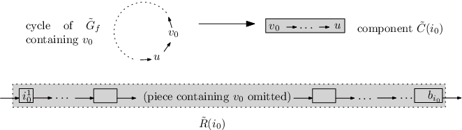
With this construction at hand, wee are now ready to prove Lemma 30. We construct a tree $\Psi_{1}(f)$ from $\tilde{G}_{f}$ , as depicted in Figure 13.

•

For $i\in\llbracket 1,r\rrbracket$ construct the left concatenation $L(i)$ . Concatenate all these pieces, by decreasing value of $i$ , to obtain a path from the vertex $a_{r}\in V_{r}$ to the vertex $1^{1}$ .
•

For $i\in\llbracket\ell,0\rrbracket\setminus\{i_{0}\}$ construct the right concatenation $R(i)$ . Construct also the components $\tilde{R}(i_{0})$ and $\tilde{C}(i_{0})$ . Concatenate $R(\ell),\dots,\tilde{R}(i_{0}),\dots,R(0)$ , by increasing value of $i$ , to obtain a path from $\ell^{1}$ to a vertex $b_{0}\in V_{0}$ .
•

Consider the distinguished path of $\tilde{C}(i_{0})$ , which goes from $v_{0}$ to $u$ . Add an edge from $1^{1}$ to $v_{0}$ , and an edge from $u$ to $0^{1}$ . This connects the previously constructed components.

Let $(T,a_{r}):=\Psi_{1}(f)$ the marked tree thus obtained. It is rooted at $b_{0}$ . It is clearly an $\mathcal{S}$ -tree (the edge that goes from $u$ to $0^{1}$ is an $\mathcal{S}$ -edge since there was in $G_{f}$ an $\mathcal{S}$ -edge going from $u$ to $v_{0}\in V_{0}$ ).

The marked tree $(T,a_{r})$ satisfies Properties $(\rm T_{1})$ and $(\rm T_{2}^{\prime})$ . The proof can be copied verbatim from the proof of Lemma 29. As before, the vertex $w_{0}$ of the marked tree $\Psi_{1}(f)=(T,a_{r})$ is $v_{0}=f(-1^{1})$ .

The meet $\ell^{1}\wedge a_{r}$ is equal to $0^{1}$ and distinct from $w_{0}$ . This is clear by construction.

The map $\Psi_{1}$ is injective. Given $(T,a_{r})$ , one recovers the graph $\tilde{C}(i_{0})$ by cutting the edge entering $w_{0}$ and the one entering $0^{1}$ on the path from $a_{r}$ to the root. Closing this piece restores a cycle of the function $f$ . Then, as in the proof of Lemma 29, we recover the remaining pieces by locating the lower records of the path from $r^{q}$ to $1^{1}$ , and of the path from the root to $\ell^{1}$ . Given the pieces, one recovers the graph $\tilde{G}_{f}$ by closing each piece containing no vertex of the form $i^{1}$ . Finally, one adds an edge from $i^{1}$ to $(i+1)^{1}$ for $i\in\llbracket\ell,-2\rrbracket$ , an edge from $i^{1}$ to $(i-1)^{1}$ for $i\in\llbracket r,1\rrbracket$ , and an edge from $-1^{1}$ to $w_{0}$ to recover the graph $G_{f}$ . This shows that $\Psi_{1}$ is injective.

The map $\Psi_{1}$ is surjective. Let $(T,r^{q})$ be a marked $\mathcal{S}$ -tree rooted at $\rho\in V_{0}$ , satisfying $(\rm T_{1})$ and $(\rm T_{2}^{\prime})$ . As above, let $w_{0}$ be the vertex that follows $1^{1}$ on the path from $r^{q}$ to the root. Assume that the meet $\ell^{1}\wedge r^{q}$ is equal to $0^{1}$ but distinct from $w_{0}$ .

On the path from $r^{q}$ to $\rho$ , one first meets $w_{0}$ and, strictly later, the meet of $\ell^{1}$ and $r^{q}$ , namely $0^{1}$ . We split the edge entering $w_{0}$ and the one entering $0^{1}$ , thus creating three connected components. One of them contains the path from $r^{q}$ to $1^{1}$ , another one contains the path from $\ell^{1}$ to $\rho$ , and the third one contains the vertex $w_{0}$ . We transform the latter into a cycle by merging the two half-edges inherited from the splitting. We call $C$ the component thus obtained.

We now consider the path going from $r^{q}$ to $1^{1}$ in the first component. We treat this part as in the proof of Lemma 29: we obtain a graph which consists of a collection of cycles and a component containing the path $r^{1}\rightarrow(r-1)^{1}\rightarrow\dots\rightarrow 1^{1}$ . On each cycle, the smallest vertex lies at a positive abscissa.

We now consider the path going from $\ell^{1}$ to the root $\rho$ . We treat this part as in the proof of Lemma 29: we obtain a graph which consists of a collection of cycles and a component containing the path $\ell^{1}\rightarrow(\ell+1)^{1}\rightarrow\dots\rightarrow-1^{1}$ . On each cycle, the smallest vertex lies at a non-positive abscissa.

Finally, add an edge from $1^{1}$ to $0^{1}$ , from $-1^{1}$ to $w_{0}$ , and let $H$ be the graph thus obtained. By construction, $H$ is the graph $G_{h}$ of a function $h:V\setminus\{0^{1}\}\rightarrow V$ satisfying (F). We check as in the proof of Lemma 29 that $h$ is an $\mathcal{S}$ -function.

By construction $v_{0}:=h(-1^{1})=w_{0}$ belongs to a cycle of the function $h$ , namely the unique cycle of the component $C$ , the source of which has abscissa at most $0$ . Thus $h$ belongs to the set of $\mathcal{S}$ -functions considered in Lemma 30.

Finally, it is clear by construction that $\Psi_{1}(h)=(T,r^{q})$ , so $\Psi_{1}$ is surjective.

Re-arranging subtrees: the bijection $\Psi_{2}$ . We say that a vertex $v\in V$ is frustrated if its in-type is not the same in $f$ and in $(T,r^{q})=\Psi_{1}(f)$ . Note that Observation 33 still holds (since Observation 34 is the analogue of Observation 28 for the components $\tilde{R}(i_{0})$ and $\tilde{C}(i_{0})$ ).

We first correct the in-types of $0^{1}$ and $v_{0}$ by exchanging the subtrees $T(0^{1})$ and $T(v_{0})$ that are attached to them in the pieces $R(0)$ and $\tilde{C}(i_{0})$ , respectively ( $0^{1}$ is an ancestor of $v_{0}$ , and these subtrees are disjoint). Let $\tilde{T}$ be the tree thus obtained. Then the in-type of $0^{1}$ in $\tilde{T}$ equals the in-type of $v_{0}$ in the function $f$ : indeed the edges contributing to these in-types are, in both cases, the edges coming from $T(v_{0})$ , plus an edge coming from $u$ , plus an edge coming from $V_{-1}$ (this edge joins $b_{-1}$ to $0^{1}$ in $\tilde{T}$ , and $-1^{1}$ to $v_{0}$ in $f$ ). Similarly, the in-type of $v_{0}$ in $\tilde{T}$ equals the in-type of $0^{1}$ in $f$ , since the edges contributing to these in-types are in both cases all edges coming from $T(0^{1})$ and the edge coming from $1^{1}$ . Finally, the operation $(T,r^{q})\mapsto(\tilde{T},r^{q})$ is an involution since the exchange of subtrees does not change the marked vertex.

We treat the path going from $r^{q}$ to $1^{1}$ in $\tilde{T}$ as in the proof of Lemma 29. That is, we exchange pairwise the trees attached to successive frustrated vertices along this path. Let $\Psi_{2}(T)$ be the marked tree obtained after performing these exchanges for all $i\in\llbracket 1,r\rrbracket$ , and let $\Psi(f)=\Psi_{2}\circ\Psi_{1}(f)$ . Since we have corrected all types, $\Psi$ satisfies Property (b). Moreover $\Psi_{2}$ is again an involution. In particular $\Psi$ is bijection, and Lemma 30 is proved.

5.3.3. Proof of Lemma 31

We assume that $v_{0}=f(-1^{1})$ belongs to the connected component of $\tilde{G}_{f}$ of source $0^{1}$ .

$\bullet$ A variation of $\tilde{G}_{f}$ : the graph $\hat{G}_{f}$ . Recall from Section 5.3.1 the construction of the graph $\tilde{G}_{f}$ , obtained by cutting into two half-edges all edges that leave a vertex of the form $i^{1}$ . If $v_{0}\not=0^{1}$ , we create a new graph $\hat{G}_{f}$ having one more cycle than $\tilde{G}_{f}$ , as follows. Let $u$ be the vertex preceding $0^{1}$ on the path that goes in $\tilde{G}_{f}$ from $v_{0}$ to $0^{1}$ . Replace the edge $u\rightarrow 0^{1}$ by an edge $u\rightarrow v_{0}$ , thus creating a new $\mathcal{S}$ -edge, a new cycle, and a new graph $\hat{G}_{f}$ . If $i_{0}$ is the smallest abscissa occurring on this cycle, then $i_{0}\leq 0$ . If $v_{0}=0^{1}$ , we let $\hat{G}_{f}=\tilde{G}_{f}$ .

Figure 14. The component containing

0^{1}

\tilde{G}_{f}

gives rise, in

\hat{G}_{f}

, to two components. One of them is a cycle containing

v_{0}

Now apply to $\hat{G}_{f}$ all the transformations applied to $\tilde{G}_{f}$ in Section 5.3.1, that led to the definition of $\Psi_{1}$ : open the cycles before or after their source (depending on the abscissa of the source), connect the resulting pieces by decreasing or increasing minima (depending again on the abscissas of the sources), and finally add an edge from $1^{1}$ to $v_{0}$ . We call the piece containing $v_{0}$ the special piece. Let $(T,a_{r}):=\Psi_{1}(f)$ be the marked tree thus obtained. It is rooted at $b_{0}$ . It is clearly a marked $\mathcal{S}$ -tree.

On checks as in Section 5.3.1 that the tree $(T,r^{q})$ satisfies $(\rm T_{1})$ and $(\rm T_{2}^{\prime})$ . Moreover, $w_{0}=v_{0}=\ell^{1}\wedge r^{q}$ , and thus the condition of Lemma 31 holds.

The map $\Psi_{1}$ is injective. One recovers the graph $\hat{G}_{f}$ in the same way one recovers $\tilde{G}_{f}$ in Section 5.3.1. If $w_{0}\not=0^{1}$ , the edge that enters $v_{0}$ in the cycle containing $v_{0}$ is then cut into two half-edges, and the outgoing half-edge is re-directed to $0^{1}$ . This gives the graph $\tilde{G}_{f}$ , from which one reconstructs $f$ easily.

We first construct from $(T,r^{p})$ a functional graph $\hat{H}$ in the same way we constructed $H$ in the proof of Lemma 29. If $w_{0}$ is distinct from $0^{1}$ , it belongs to a cycle of $\hat{H}$ : we cut the edge of this cycle entering $w_{0}$ into two half-edges, and redirect the outgoing half-edge onto $0^{1}$ .

The graph $H$ thus obtained is the graph $G_{h}$ of a function $h:V\setminus\{0^{1}\}\rightarrow V$ satisfying (F), which is checked as before to be an $\mathcal{S}$ -function.

By construction $h(-1^{1})=w_{0}$ belongs to the connected component containing $0^{1}$ in $\tilde{G}_{h}$ , so that $h$ belongs to the set of $\mathcal{S}$ -functions considered in Lemma 31.

Finally, it is clear by construction that $\Psi_{1}(h)=(T,r^{q})$ , so $\Psi_{1}$ is surjective.

$\bullet$ Re-arranging subtrees: the bijection $\Psi_{2}$ . The only vertices that are likely to be frustrated are the lower records of the path going from $a_{r}$ to $1^{1}$ , and the vertices $0^{1}$ and $v_{0}$ . These two vertices belong to the path going from $\ell^{1}$ to the root. We first correct their in-types by swapping the subtrees $T(0^{1})$ and $T(v_{0})$ that are attached to them in their respective pieces. Let $\tilde{T}$ be the tree thus obtained. Then the in-type of $0^{1}$ in $\tilde{T}$ equals the in-type of $v_{0}$ in the function $f$ : indeed the edges contributing to these in-types are, in both cases, the edges coming from $T(v_{0})$ , plus an edge coming from $V_{-1}$ (this edge joins $b_{-1}$ to $0^{1}$ in $\tilde{T}$ , and $-1^{1}$ to $v_{0}$ in $f$ ). Similarly, the in-type of $v_{0}$ in $\tilde{T}$ equals the in-type of $0^{1}$ in $f$ , since edges contributing to these in-types are, in both cases, the edges coming from $T(0^{1})$ , plus an edge coming from $1^{1}$ , plus an edge coming from a vertex having the same asbcissa as $u$ (this edge joins $u$ to $0^{1}$ in $f$ ; in $\tilde{T}$ , it joins $u$ to $v_{0}$ , unless $u$ is the minimum on the cycle containing $v_{0}$ . In this case, the abscissa of $u$ is $i_{0}$ , $v_{0}$ is a source in $\tilde{T}$ , and is the endpoint of another sink of abscissa $i_{0}$ ). Finally, the map $(T,a_{r})\mapsto(\tilde{T},a_{r})$ is again an involution.

The frustrated vertices lying on the path going from $a_{r}$ to $1^{1}$ in $\tilde{T}$ are treated as before, by exchanging the trees attached to successive frustrated vertices. Let $\Psi_{2}(T)$ be the marked tree obtained after performing these exchanges for all $i\in\llbracket 1,r\rrbracket$ . As before $\Psi_{2}$ is an involution, so that $\Psi:=\Psi_{2}\circ\Psi_{1}$ is a bijection. It satisfies Property (b), and Lemma 31 is proved.

5.4. Proof of Proposition 26

We now assume that $v_{0}=f(-1^{1})$ belongs to $W_{i_{0}}$ , with $i_{0}\geq 1$ . We first perform some surgery on the piece $L(i_{0})$ containing $v_{0}$ .

$\bullet$ Surgery on $L(i_{0})$ : the graphs $\tilde{L}(i_{0}),A(i_{0})$ and $B(i_{0})$ .

Recall that $L(i_{0})$ consists of a path going from the vertex $a_{i_{0}}$ to the vertex $i_{0}^{1}$ , to which trees are attached. One of these trees contains the vertex $v_{0}$ , and we let $v$ be the attachment point of this tree on the path. Note that we have $a(v)\geq i_{0}\geq 1$ , and in particular $v\neq v_{0}$ since $v_{0}\in V_{0}$ .

We now define two other vertices $x_{0}$ , $y_{0}$ as follows (Figure 16). Consider the path of $L(i_{0})$ going from $v_{0}$ to $v$ , and let us distinguish two cases. If there exists a vertex of negative abscissa along this path, we let $x_{-1}$ (resp. $y_{-1}$ ) be the first (resp. last) vertex of $V_{-1}$ encountered on the path from $v_{0}$ to $v$ , and we let $x_{0}$ (resp. $y_{0}$ ) be the vertex preceding $x_{-1}$ (resp. following $y_{-1}$ ) on the path. Note that since $\max\mathcal{S}=1$ and $\min\mathcal{S}=-1$ , the vertices $x_{-1}$ and $y_{-1}$ are well defined; moreover, $x_{0}$ and $y_{0}$ belong to $V_{0}$ . Now, cut the edge between $x_{0}$ and $x_{-1}$ , and the edge between $y_{-1}$ and $y_{0}$ . Among the three connected components thus created, we call $\tilde{L}(i_{0})$ the one containing $v$ , we call $A(i_{0})$ the one containing $x_{-1}$ , and we call $B(i_{0})$ the one containing $v_{0}$ . If all the vertices on the path from $v_{0}$ to $v$ have a nonnegative abscissa, we let $\tilde{L}(i_{0}):=L(i_{0})$ , $A(i_{0}):=B(i_{0}):=\varnothing$ , and $y_{0}:=x_{0}:=v_{0}$ . In this case, the vertices $x_{-1}$ and $y_{-1}$ are not defined.

By construction, we have the following analogue of Observation 27.

Observation 35.

Any vertex of the graph $\tilde{L}(i_{0})\cup A(i_{0})\cup B(i_{0})$ , distinct from $v_{0}$ , $y_{0}$ and $x_{-1}$ and from the lower records of the path going from $a_{i_{0}}$ to $i_{0}^{1}$ , has the same in-type in this graph and in the function $f$ .

We now proceed with the description of the bijection, depicted in Figure 17. We perform the following operations.

•

For $i\in\llbracket 0,r\rrbracket$ , construct the left concatenation $L(i)$ . Construct the graph $\tilde{L}(i_{0})$ from $L(i_{0})$ , and concatenate the pieces

$L(r),L(r-1),\dots,L(i_{0}-1),\tilde{L}(i_{0}),L(i_{0}+1),\dots,L(1),L(0)$

to obtain a path from the vertex $a_{r}\in V_{r}$ to the vertex $0^{1}$ . Note that $y_{0}$ belongs to a subtree attached to this path.
•

For $i\in\llbracket\ell,-1\rrbracket$ construct the right concatenation $R(i)$ . Concatenate all these pieces by increasing value of $i$ , to obtain a path from $\ell^{1}$ to the vertex $b_{-1}\in V_{-1}$ .
•

Add an edge from $b_{-1}$ to $y_{0}$ . This connects the two previously constructed components.
•

If $A(i_{0})\neq\varnothing$ (equivalently, if $B(i_{0})\neq\varnothing)$ , add an edge from $0^{1}$ to $x_{-1}$ , and an edge from $y_{-1}$ to $v_{0}$ . This connects the components $A(i_{0})$ and $B(i_{0})$ to the previously constructed tree.

Let $\Psi_{1}(f):=(T,a_{r})$ be the marked tree thus obtained. It is rooted at $x_{0}$ if $A(i_{0})\neq\varnothing$ and at $0^{1}$ otherwise. It is easily checked to be an $\mathcal{S}$ -tree.

As in the previous proofs, we are first going to show that the mapping $\Psi_{1}$ is a bijection between the sets described in Proposition 26. Then we will describe another bijection, $\Psi_{2}$ , such that $\Psi_{2}\circ\Psi_{1}$ satisfies Property (b), which $\Psi_{1}$ lacks.

The marked tree $(T,a_{r})$ satisfies Properties $(\rm T_{1})$ and $(\rm T_{2}^{\prime\prime})$ . The fact that $T$ satisfies $(\rm T_{1})$ is proved as in the proof of Lemma 29. The meet $\ell^{1}\wedge a_{r}$ is equal to $v$ , and since $i_{0}\geq 1$ , it appears weakly before the vertex $1^{1}$ on the path from $a_{r}$ to the root. Hence the first part of $(\rm T_{2}^{\prime\prime})$ holds. As underlined above, the abscissa of $v$ , being at least $i_{0}$ , is positive. The arguments proving the second part of $(\rm T_{2}^{\prime\prime})$ are the same as those proving $(\rm T_{2}^{\prime})$ in Lemma 29 (the concatenation of $R(\ell),\ldots,R(-1)$ is the same in both proofs). Finally, all vertices on the path from $a_{r}$ to $0^{1}$ have a nonnegative abscissa. Hence either $0^{1}$ is the root of the tree, and there are no vertices of negative abscissa on the path joining $a_{r}$ to the root, or $0^{1}$ is not the root, in which case there are such vertices, and $0^{1}$ precedes the first of them (which is $x_{-1}$ ). This establishes the last part of $(\rm T_{2}^{\prime\prime})$ .

The map $\Psi_{1}$ is injective. Let us start from the marked tree $\Psi_{1}(f)=(T,a_{r})$ and reconstruct $f$ . First, on the path going from $\ell^{1}$ to the root, we cut the edge that leaves the last vertex of abscissa $-1$ , denoted $b_{-1}$ . The other endpoint of this edge is $y_{0}$ . By cutting the path that goes from $a_{r}$ to $0^{1}$ after each vertex of the form $i^{1}$ , we recover the graphs $L(i)$ , for $i\in\llbracket 0,r\rrbracket\setminus\{i_{0}\}$ , and the graph $\tilde{L}(i_{0})$ . Similarly, by cutting, in the path that goes from $\ell^{1}$ to $b_{-1}$ , each edge that enters a vertex of the form $i^{1}$ , we recover the graphs $R(i)$ , for ${i\in\llbracket\ell,-1\rrbracket}$ . If $0^{1}$ is not the root of the tree, we recover moreover the vertices $x_{-1}$ (it follows $0^{1}$ on its path to the root) and $y_{-1}$ (the last vertex of negative abscissa on this path), so that we can reconstruct the graphs $A(i_{0})$ and $B(i_{0})$ . In all cases, we can then reconstruct the graph $L(i_{0})$ . We then proceed as in the proof of Lemma 29: in each $L(i)$ (resp $R(i)$ ), locate each left-to-right (resp. right-to-left) lower record, and split the edges entering (resp. leaving) each of them. Then close the pieces whose root is not of the form $i^{1}$ to recover a cycle of the original function $f$ . One thus recovers the graph $\tilde{G}_{f}$ . Finally, add an edge from $i^{1}$ to $(i+1)^{1}$ for $i\in\llbracket\ell,-2\rrbracket$ , an edge from $i^{1}$ to $(i-1)^{1}$ for $i\in\llbracket r,1\rrbracket$ , and an edge from $-1^{1}$ to $v_{0}$ (the vertex that follows $y_{-1}$ on its path to the root) to recover the graph $G_{f}$ .

The map $\Psi_{1}$ is surjective. Let $(T,r^{q})$ be a marked $\mathcal{S}$ -tree rooted at $\rho\in V_{0}$ , satisfying $(\rm T_{1})$ and $(\rm T_{2}^{\prime\prime})$ . Denote $v:=\ell^{1}\wedge r^{q}$ . By $(\rm T_{2}^{\prime\prime})$ , we have $a(v)\geq 1$ .

Consider the path going from $\ell^{1}$ to $v$ in $T$ , and let $b_{-1}$ be the last vertex of negative abscissa on this path, and $y_{0}$ the next vertex on this path. Note that $b_{-1}$ (resp. $y_{0}$ ) has abcissa $-1$ (resp. $0$ ). Split the edge joining $b_{-1}$ to $y_{0}$ . This gives two connected components, one containing the path from $r^{q}$ to the root (including the vertex $v$ ), the other the path from $\ell^{1}$ to $b_{-1}$ .

Now visit the path going $b_{-1}$ to $\ell^{1}$ (in this “wrong” direction). Lower records on this path are called sinks, and vertices preceding the sinks (in the same “wrong” direction) are called sources (we consider $\ell^{1}$ as a source). We now split all edges between sinks and sources, and thus obtain a number of pieces. By $(\rm T_{2}^{\prime\prime})$ , each vertex $i^{1}$ for $i\in\llbracket\ell,-1\rrbracket$ is the source and the sink of a piece. Take all the pieces containing a vertex $i^{1}$ , for $i\leq-1$ , and concatenate them by adding an edge from $i^{1}$ to $(i+1)^{1}$ for $i\in\llbracket\ell,-2\rrbracket$ . In the remaining pieces, merge the two extremal half-edges to form a cycle.

We now describe a step of the reverse bijection that applies only if $0^{1}$ is not the root of $T$ . In that case, $(\rm T_{2}^{\prime\prime})$ implies that the vertex $0^{1}$ belongs to the path from $r^{q}$ to the root, and is followed by a vertex of $V_{-1}$ , say $x_{-1}$ . Let $y_{-1}$ be the last vertex of $V_{-1}$ on the path from $0^{1}$ to the root, and let $v_{0}\in V_{0}$ be the vertex following it. We now split the edge between $0^{1}$ and $x_{-1}$ , and the edge between $y_{-1}$ and $v_{0}$ . We call $\tilde{A}$ and $\tilde{B}$ the connected components containing $x_{-1}$ and $v_{0}$ after the splitting, respectively. We re-connect the components $\tilde{A}$ and $\tilde{B}$ to the connected component of $r^{q}$ by adding an edge from $x_{0}$ to $x_{-1}$ and from $y_{-1}$ to $y_{0}$ . This concludes the step that is specific to the case where $0^{1}$ is not the root of $T$ . Otherwise, we denote $\tilde{A}:=\tilde{B}:=\varnothing$ , and $y_{0}=x_{0}:=v_{0}$ .

We now consider the path going from $r^{q}$ to $0^{1}$ . Lower records on this path are called sources, and vertices preceding the sources are called sinks (we consider $0^{1}$ as a sink). We now split each edge that enters a source of the path, and thus obtain a number of pieces. By $(\rm T_{1})$ and $(\rm T_{2}^{\prime\prime})$ , each vertex $i^{1}$ for $i\in\llbracket 0,r\rrbracket$ is the source and the sink of a piece. Take all the pieces containing a vertex of the form $i^{1}$ , for $i\geq 0$ , and concatenate them by adding an edge from $i^{1}$ to $(i-1)^{1}$ for $i\in\llbracket 1,r\rrbracket$ . Transform each of the remaining pieces into a cycle by merging the two extremal half-edges. Finally, add an edge from $-1^{1}$ to $v_{0}$ .

Let $H$ be the graph thus obtained. By construction, $H$ is the graph $G_{h}$ of a function $h:V\setminus\{0^{1}\}\rightarrow V$ satisfying (F). One easily checks that $h$ is an $\mathcal{S}$ -function, using the same arguments as in the proof of Lemma 29, plus the facts that $h(y_{-1})=y_{0}\in V_{0}$ and $h(x_{0})=x_{-1}\in V_{-1}$ .

Let us now prove that $h$ satisfies the condition of Proposition 26. By construction, the source of the component of $\tilde{G}_{h}$ containing $v_{0}=h(-1^{1})$ is the last lower record encountered (weakly) before $v$ on the path from $r^{q}$ to $v$ in $T$ . By $(\rm T_{2}^{\prime\prime})$ this source appears (weakly) before $1^{1}$ , and since $1^{1}$ is a lower record by $(\rm T_{1})$ , the abscissa of this source is at least $1$ . In other words, we have $v_{0}\in\cup_{i=1}^{r}W_{i}$ , the sets $W_{i}$ being understood with respect with the function $h$ .

Finally, note that all abscissas are nonnegative on the paths from $y_{0}$ to $v$ and from $v_{0}$ to $x_{0}$ . This implies that $\tilde{A}$ and $\tilde{B}$ coincide with the pieces $A(i_{0})$ and $B(i_{0})$ which one would build from the function $h$ . From that it is clear that $\Psi_{1}(h)=(T,r^{q})$ , so that $\Psi_{1}$ is surjective.

$\bullet$ Re-arranging subtrees: the bijection $\Psi_{2}$ . We say that a vertex $v\in V$ is frustrated if its in-type is not the same in $f$ and in $(T,a_{r})=\Psi_{1}(f)$ . We claim that the vertices belonging to $\cup_{i=\ell}^{-1}W_{i}$ are not frustrated. This is a direct consequence of Observation 28 and of the fact that to concatenate $R(i-1)$ to $R(i)$ , for $i\in\llbracket\ell+1,-1\rrbracket$ , we add a new incoming edge to the vertex $i^{1}$ coming from $V_{i-1}$ , which compensates the deletion of the edge $(i-1)^{1}\rightarrow i^{1}$ in the construction of $\tilde{G}_{f}$ from $f$ . Similarly, Observations 27 and 35 give:

Observation 36.

Any vertex of $\cup_{i=0}^{r}W_{i}$ distinct from $v_{0},y_{0},x_{-1}$ , and from the lower records of the path from $r^{q}$ to $0^{1}$ is not frustrated.

In fact, $y_{0}$ is not frustrated: indeed, the edge coming from $b_{-1}$ in $T$ compensates either the loss of the edge coming from $y_{-1}$ in $L(i_{0})$ (if $y_{0}\neq v_{0}$ ) or the loss of the edge coming from $-1^{1}$ in $f$ (if $y_{0}=v_{0})$ , and since $y_{0}$ does not belong to the distinguished path of $L(i_{0})$ , Observation 27 enables us to conclude. Similarly, $x_{-1}$ (if it exists) is not frustrated, since the edge coming from $0^{1}$ in $T$ compensates the edge coming from $x_{0}$ in $L(i_{0})$ . Finally, $v_{0}$ is not frustrated either: either it is equal to $y_{0}$ (if $0^{1}$ is the root of $T$ ), or the edge coming from $y_{-1}$ in $T$ compensates the loss of the edge coming from $-1^{1}$ in $f$ . Therefore, we can strengthen our previous observation as follows.

Observation 37.

Any vertex of $\cup_{i=0}^{r}W_{i}$ distinct from the lower records of the path from $r^{q}$ to $0^{1}$ is not frustrated.

We correct the in-types of these sources by a second map $\Psi_{2}$ . We proceed as in the proof of Theorem 9 in Section 3, by exchanging the subtrees attached to adjacent frustrated vertices. Let $\Psi_{2}(T,r^{q})$ be the tree thus obtained, and $\Psi(f)=\Psi_{2}\circ\Psi_{1}(f)$ . One again, $\Psi_{2}$ is an involution. In particular $\Psi$ is bijection, which satisfies Property (b) thanks to the construction $\Psi_{2}$ . Proposition 26 is proved.

6. Enumeration of general embedded trees

In this section, we prove the enumerative results of Section 2 in the case $\ell<0$ . These results follow from the bijection of Theorem 24, combined with the enumeration of $\mathcal{S}$ -functions (which remains an elementary exercise). We also need to relate the $\mathcal{S}$ -trees occurring in Theorem 24 to the $\mathcal{S}$ -embedded Cayley trees of Section 2. This is done in the following lemma. We adopt the same notation as in the previous section: $V=\cup_{i=\ell}^{r}V_{i}$ with $V_{i}=\{i^{1},\ldots,i^{n_{i}}\}$ , and $\mathcal{S}\subset{\mathbb{Z}}$ satisfies $\min\mathcal{S}=-1$ and $\max\mathcal{S}=1$ . The type distribution of a tree is the collection of numbers $n(i,s,\mbox{\boldmath$c$})$ (with $i\in\llbracket 0,r\rrbracket$ , $s\in\mathcal{S}$ and $\mbox{\boldmath$c$}\in{\mathbb{N}}^{3}$ ) giving the number of vertices of type $(i;s;\mbox{\boldmath$c$})$ .

Lemma 38.

The number of $\mathcal{S}$ -embedded Cayley trees having a prescribed type distribution is

\frac{1}{n_{\ell}n_{r}}\frac{n!}{\prod_{i=\ell}^{r}(n_{i}-1)!}

times the number of marked $\mathcal{S}$ -trees satisfying Conditions $(\rm T_{1})$ and $(\rm T_{2})$ of Theorem 24 and having the same type distribution (as always, $(n_{\ell},\ldots,n_{r})$ denotes the profile of the tree, and $n$ its size).

Proof.

Equivalently, we want to prove that the number of $\mathcal{S}$ -embedded Cayley trees having a prescribed type distribution and two marked vertices, one at abscissa $\ell$ and the other at abscissa $r$ , is

\frac{n!}{\prod_{i}(n_{i}-1)!}

times the number of marked $\mathcal{S}$ -trees satisfying $(\rm T_{1})$ and $(\rm T_{2})$ and having the same type distribution. We will construct a 1-to- $n!/\prod_{i}(n_{i}-1)!$ correspondence between marked $\mathcal{S}$ -trees satisfying $(\rm T_{1})$ and $(\rm T_{2})$ and doubly marked $\mathcal{S}$ -embedded Cayley trees, preserving the type distribution.

Let $(T,r^{q})$ be a marked $\mathcal{S}$ -tree on $V$ satisfying $(\rm T_{1})$ and $(\rm T_{2})$ . Let us mark, in addition, the vertex $\ell^{1}$ . For $\ell\leq i\leq r$ , let us rename the vertex $i^{1}$ by $i^{k}$ , for a $k$ chosen in $\{1,\ldots,n_{i}\}$ ; conversely, let us rename $i^{k}$ by $i^{1}$ . This gives an arbitrary $\mathcal{S}$ -tree $T_{1}$ , rooted at a vertex of $V_{0}$ , with two marked vertices, one at abscissa $\ell$ and one at abscissa $r$ . This tree may or may not satisfy $(\rm T_{1})$ and $(\rm T_{2})$ . The number of different trees $T_{1}$ that can be constructed from $T$ in such a way is $\prod_{i=\ell}^{r}n_{i}$ . The tree $T$ can be recovered from $T_{1}$ by restoring vertex names: indeed, the vertex $\ell^{1}$ in $T$ is at the position of the marked vertex of abscissa $\ell$ in $T_{1}$ , and the position of $i^{1}$ in $T$ , for $i>\ell$ , is prescribed by $(\rm T_{1})$ and $(\rm T_{2})$ .

Let us now assign labels from $\{1,\ldots,n\}$ , with $n=\sum_{i}n_{i}$ , to the vertices of $T_{1}$ , in such a way that the labels $a$ and $b$ assigned to $i^{k}$ and $i^{p}$ satisfy $a<b$ if $k<p$ . There are $n!/\prod_{i}n_{i}!$ ways to do so. Finally, erase all names $i^{k}$ from the tree, for all $i$ and $k$ . This gives an arbitrary rooted $\mathcal{S}$ -embedded Cayley tree $T_{2}$ , with a marked vertex at abscissa $\ell$ and one at abscissa $r$ . The tree $T_{1}$ can be recovered from $T_{2}$ by renaming the vertices of abscissa $i$ with $i^{1},\ldots,i^{n_{i}}$ in the unique way that is consistent with the order on labels: if two vertices of labels $a$ and $b$ , with $a<b$ , lie at abscissa $i$ , then their names $i^{k}$ and $i^{p}$ must satisfy $k<p$ .

The marked $\mathcal{S}$ -tree $T$ has given rise to $n!/\prod_{i}(n_{i}-1)!$ doubly marked embedded trees $T_{2}$ . Moreover, $T_{2}$ , $T_{1}$ and $T$ have the same type distribution. The result follows.

In what follows, we count trees by counting functions, using the correspondence of Theorem 24. When we prescribe the types of vertices, or the number of vertices of a certain type, we assume as in Section 4 that the natural compatibility conditions hold.

Recall that Theorem 3 is already proved, even when $\ell<0$ , thanks to the fourth remark that follows its statement.

6.1. The profile of $\mathcal{S}$ -ary trees: proof of Theorem 4

We argue as in Section 4.2. The number of $\mathcal{S}$ -ary trees of vertical profile $(n_{\ell},\ldots,n_{r})$ is obtained by divising by $n!$ the number of injective $\mathcal{S}$ -embedded Cayley trees with the same profile. By Lemma 38, the number of injective $\mathcal{S}$ -embedded Cayley trees having vertical profile $(n_{\ell},\ldots,n_{r})$ is $n!/n_{\ell}/n_{r}/\prod_{i}(n_{i}-1)!$ times the number of marked injective $\mathcal{S}$ -trees satisfying $(\rm T_{1})$ and $(\rm T_{2})$ . By Theorem 24 (and in particular Property (b)), the number of such trees is also the number of $\mathcal{S}$ -functions from $V\setminus\{0^{1}\}$ satisfying (F) that are injective on each $V_{i}$ . This number is given by the following lemma. Theorem 4 follows, in the case $\ell<0$ .

Lemma 39.

The number of $\mathcal{S}$ -functions from $V\setminus\{0\}$ , injective on each $V_{i}$ and satisfying $(\rm F)$ is

n_{0}\,{\sum_{s\in\mathcal{S}}n_{-s}\choose n_{0}-1}\prod_{i=\ell\atop i\not=0}^{r}{\sum_{s\in\mathcal{S}}n_{i-s}-1\choose n_{i}-1}\prod_{i=\ell}^{r}(n_{i}-1)!.

Proof.

We proceed as in the proof of Lemma 17. For $i\not\in\{0,-1\}$ , we choose the (distinct) images of the elements of $V_{i}\setminus\{i^{1}\}$ in the set $\cup_{s}V_{i-s}\setminus\{f(i^{1})\}$ , where $f(i^{1})=(i-1)^{1}$ if $i>1$ and $f(i^{1})=(i+1)^{1}$ if $i<0$ . There are ${\sum_{s}n_{i-s}-1\choose n_{i}-1}(n_{i}-1)!$ ways to do so.

For $i=0$ , we choose the (distinct) images of the elements of $V_{0}\setminus\{0^{1}\}$ in the set $\cup_{s}V_{-s}$ . There are ${\sum_{s}n_{-s}\choose n_{0}-1}(n_{0}-1)!$ ways to do so.

For $i=-1$ , we first choose the image $v_{0}$ of $-1^{1}$ in the set $V_{0}$ : there are $n_{0}$ ways to do so. Then, we choose the (distinct) images of elements of $V_{-1}\setminus\{-1^{1}\}$ in the set $\cup_{s}V_{-1-s}\setminus\{v_{0}\}$ . There are ${\sum_{s}n_{-1-s}-1\choose n_{-1}-1}(n_{-1}-1)!$ ways to do so.

6.2. The out-types of $\mathcal{S}$ -embedded Cayley trees: proof of Theorem 5

We argue as in Section 4.3. By Lemma 38 and Theorem 24 (in particular Property (a)), the number of $\mathcal{S}$ -embedded Cayley trees having $n(i,s)$ non-root vertices of out-type $(i;s)$ is $n!/n_{\ell}/n_{r}/\prod_{i}(n_{i}-1)!$ times the number of $\mathcal{S}$ -functions from $V\setminus\{0^{1}\}$ to $V$ satisfying (F) and having the same distribution of out-types. This number is given by the following lemma. Theorem 5 follows, in the case $\ell<0$ .

Lemma 40.

$1$ . The number of $\mathcal{S}$ -functions from $V\setminus\{0^{1}\}$ to $V$ satisfying $(\rm F)$ and in which each $v\in V$ has a prescribed out-type $(i_{v};s_{v})$ is, assuming compatibility,

n_{\ell}n_{r}\prod_{i=\ell}^{r}n_{i}^{c(i)-1},

where $c(i)$ is the number of vertices whose image lies in $V_{i}$ :

c(i)=\sharp\{v\in V:i_{v}-s_{v}=i\}.

$2$ . Let $n(i,s)$ be non-negative integers, for $i\in\llbracket\ell,r\rrbracket$ and $s\in\mathcal{S}$ , satisfying the compatibility conditions of an out-type distribution. The number of $\mathcal{S}$ -functions from $V\setminus\{0^{1}\}$ to $V$ satisfying $(\rm F)$ and in which, for all $i\in\llbracket\ell,r\rrbracket$ and $s\in\mathcal{S}$ , exactly $n(i,s)$ vertices have out-type $(i;s)$ is

\frac{n_{\ell}n_{r}\prod\limits_{i=\ell}^{r}(n_{i}-1)!\prod\limits_{i=\ell}^{r}n_{i}^{c(i)-1}\prod\limits_{i=\ell}^{-1}n(i,-1)\prod\limits_{i=1}^{r}n(i,1)}{\prod\limits_{i,s}n(i,s)!},

where $c(i)$ is the number of vertices whose image lies in $V_{i}$ :

c(i)=\sum_{s}n(i+s,s).

Proof.

We proceed as in the proof of Lemma 18.

1. We first choose the images of the $c(i)$ vertices whose image is in $V_{i}$ , for $i\in\{\ell,r\}$ . There are $n_{i}^{c(i)}$ possible choices. For $i\in\llbracket 0,r-1\rrbracket$ (resp. $i\in\llbracket\ell+1,-1\rrbracket$ ) we only choose in $V_{i}$ the images of the vertices different from $(i+1)^{1}$ (resp. $(i-1)^{1}$ ). There are $n_{i}^{c(i)-1}$ possible choices.

2. We first choose the out-type of every vertex, and then apply the previous result. For all $i$ and $s$ , we must choose the $n(i,s)$ vertices of $V_{i}$ that have out-type $(i;s)$ , keeping in mind that $i^{1}$ has out-type $(i;1)$ for $i\geq 1$ , out-type $(i;-1)$ for $i\leq-1$ , and out-type $(0;\varepsilon)$ for $i=0$ . Thus the number of ways to assign the out-types is

\frac{(n_{0}-1)!}{\prod\limits_{s}n(0,s)!}\prod_{i=\ell}^{-1}\frac{(n_{i}-1)!}{(n(i,-1)-1)!\prod\limits_{s\not=-1}n(i,s)!}\prod_{i=1}^{r}\frac{(n_{i}-1)!}{(n(i,1)-1)!\prod\limits_{s\not=1}n(i,s)!}.

The lemma follows.

6.3. The out-types of $\mathcal{S}$ -ary trees: Proof of Theorem 6

We argue as in Section 4.4. By Lemma 38 and Theorem 24, the number of $\mathcal{S}$ -ary trees having $n(i,s)$ non-root vertices of out-type $(i;s)$ is $1/n_{\ell}/n_{r}/\prod_{i}(n_{i}-1)!$ times the number of $\mathcal{S}$ -functions from $V\setminus\{0^{1}\}$ to $V$ satisfying (F) that are injective on each $V_{i}$ and have the same distribution of out-types. This number is given by the second part of the following lemma. Theorem 6 follows, in the case $\ell<0$ .

Lemma 41.

\frac{1}{\prod\limits_{i=\ell+1}^{r-1}n_{i}}\prod_{i,s}n(i,s)!{{n_{i-s}}\choose{n(i,s)}},

where $n(i,s)$ is the number of vertices of out-type $(i,s)$ .

$2$ . Let $n(i,s)$ be non-negative integers, for $i\in\llbracket\ell,r\rrbracket$ and $s\in\mathcal{S}$ , satisfying the compatibility conditions of an out-type distribution. The number of $\mathcal{S}$ -functions from $V\setminus\{0^{1}\}$ to $V$ , injective on each $V_{i}$ , satisfying $(\rm F)$ and in which, for all $i\in\llbracket\ell,r\rrbracket$ and $s\in\mathcal{S}$ , exactly $n(i,s)$ vertices have out-type $(i;s)$ is

\frac{\prod\limits_{i=\ell}^{r}(n_{i}-1)!\prod\limits_{i=\ell}^{-1}n(i,-1)\prod\limits_{i=1}^{r}n(i,1)}{\prod\limits_{i=\ell+1}^{r-1}n_{i}}\prod_{i,s}{n_{i-s}\choose n(i,s)}.

Proof.

We proceed as in the proof of Lemma 19.

1. For

•

$i\in\llbracket-1,0\rrbracket$ and $s\in\mathcal{S}$ ,
•

or $i\in\llbracket\ell,-2\rrbracket$ , and $s\in\mathcal{S}\setminus\{-1\}$ ,
•

or $i\in\llbracket 1,r\rrbracket$ , and $s\in\mathcal{S}\setminus\{1\}$ ,

we choose in $V_{i-s}$ the (distinct) images of the $n(i,s)$ vertices having out-type $(i,s)$ . There are ${n_{i-s}\choose n(i,s)}n(i,s)!$ ways to do so.

When $i\in\llbracket 1,r\rrbracket$ and $s=1$ , we choose in $V_{i-1}\setminus\{(i-1)^{1}\}$ the images of the $n(i,s)-1$ vertices different from $i^{1}$ having out-type $(i,1)$ . There are

{n_{i-1}-1\choose n(i,1)-1}(n(i,1)-1)!={n_{i-1}\choose n(i,1)}\frac{n(i,1)!}{n_{i-1}}

ways to do so.

When $i\in\llbracket\ell,-2\rrbracket$ and $s=-1$ , we choose in $V_{i+1}\setminus\{(i+1)^{1}\}$ the images of the $n(i,s)-1$ vertices different from $i^{1}$ having out-type $(i,-1)$ . There are

{n_{i+1}-1\choose n(i,-1)-1}(n(i,-1)-1)!={n_{i+1}\choose n(i,-1)}\frac{n(i,-1)!}{n_{i+1}}

ways to do so.

This concludes the proof of the first result.

2. The argument used to prove the second part of Lemma 40 can be copied verbatim.

6.4. The in-types: Proof of Theorem 7

Assume $\mathcal{S}=\llbracket-1,1\rrbracket$ . We argue as in Section 4.5. By Lemma 38 and Theorem 24 (in particular Property (b) of this theorem), the number of $\mathcal{S}$ -embedded Cayley trees having $n(i,\mbox{\boldmath$c$})$ vertices of in-type $(i;\mbox{\boldmath$c$})$ is $n!/n_{\ell}/n_{r}/\prod_{i}(n_{i}-1)!$ times the number of $\mathcal{S}$ -functions from $V\setminus\{0^{1}\}$ to $V$ satisfying (F) and having the same distribution of in-types. This number is given by the second part of the following lemma. Theorem 7 follows, in the case $\ell<0$ .

Lemma 42.

Let $\mathcal{S}=\llbracket-1,1\rrbracket$ .
$1$ . The number of $\mathcal{S}$ -functions $f$ from $V\setminus\{0^{1}\}$ to $V$ satisfying Conditions $(\rm F)$ , except maybe the condition $f(-1^{1})\in V_{0}$ , and in which each $v\in V$ has a prescribed in-type $(i_{v};\mbox{\boldmath$c$}_{v})$ is, assuming compatibility,

n_{-1}\,\frac{\prod\limits_{i=\ell}^{r}(n_{i}-1)!}{\prod\limits_{b\geq 0,s}b!^{n_{s}(b)}}\prod_{i=\ell+1}^{-1}c_{i^{1}}^{-1}\prod_{i=0}^{r-1}c_{i^{1}}^{1},

where $n_{s}(b)$ is the number of vertices $v$ that have exactly $b$ pre-images at abscissa $a(v)+s$ :

n_{s}(b)=\sharp\{v\in V:c_{v}^{s}=b\}.

$2.$ Let $n(i,\mbox{\boldmath$c$})$ be non-negative integers, for $i\in\llbracket\ell,r\rrbracket$ and $\mbox{\boldmath$c$}\in{\mathbb{N}}^{3}$ , satisfying the compatibility conditions of an in-type distribution. The number of $\mathcal{S}$ -functions from $V\setminus\{0^{1}\}$ to $V$ satisfying $(\rm F)$ and in which, for all $i\in\llbracket\ell,r\rrbracket$ and $\mbox{\boldmath$c$}\in{\mathbb{N}}^{3}$ , exactly $n(i,\mbox{\boldmath$c$})$ vertices have in-type $(i;\mbox{\boldmath$c$})$ is

\frac{n_{\ell}n_{r}\prod\limits_{i=\ell}^{r}(n_{i}-1)!^{2}}{\prod\limits_{i,\mbox{\scriptsize\boldmath$c$}}n(i,\mbox{\boldmath$c$})!\prod\limits_{b\geq 0,s}b!^{n_{s}(b)}}\prod\limits_{i=\ell}^{-1}n(i,-1)\prod\limits_{i=1}^{r}n(i,1),

where $n_{s}(b)$ is the number of vertices $v$ that have exactly $b$ pre-images at abscissa $a(v)+s$ , and $n(i,1)$ is the number of vertices of out-type $(i;1)$ . Equivalently,

\displaystyle n_{s}(b)=\sum_{i}\sum_{\mbox{\scriptsize\boldmath$c$}:c^{s}=b}n(i,\mbox{\boldmath$c$}),\quad\quad n(i,1)=\sum_{\mbox{\scriptsize\boldmath$c$}}c^{1}n(i-1,\mbox{\boldmath$c$}).

Proof.

We proceed as in the proof of Lemma 20.

1. Let us first choose the images of the $n_{-1}$ vertices of $V_{-1}$ . Exactly $c_{(-1-s)^{k}}^{s}$ of them have image $(-1-s)^{k}$ , for all $s$ and $k$ . For $i\in\llbracket\ell,r\rrbracket\setminus\{-1\}$ , let us choose the images of the $n_{i}-1$ vertices of $V_{i}\setminus\{i^{1}\}$ . Exactly $c_{(i-s)^{k}}^{s}-{\bf 1}_{s=1=k=1,i>0}-{\bf 1}_{s=-1,k=1,i<-1}$ of them have image $(i-s)^{k}$ , for all $s$ and $k$ . The first result follows.

2. We first focus on functions that satisfy Conditions (F), except maybe the condition $f(-1^{1})\in V_{0}$ . Let us first prescribe the in-type $(i;\mbox{\boldmath$c$}_{i^{1}})$ of all vertices of the form $i^{1}$ , for all $i$ , and the number $\tilde{n}(i;\mbox{\boldmath$c$})$ of vertices of $V_{i}\setminus\{i^{1}\}$ having in-type $(i;\mbox{\boldmath$c$})$ , for all $\mbox{\boldmath$c$}\in{\mathbb{N}}^{3}$ . Clearly,

\tilde{n}(i,\mbox{\boldmath$c$})=n(i,\mbox{\boldmath$c$})-{\bf 1}_{\mbox{\scriptsize\boldmath$c$}=\mbox{\scriptsize\boldmath$c$}_{i^{1}}}.

The number of ways to assign types to vertices of $V_{i}\setminus\{i^{1}\}$ is

\frac{(n_{i}-1)!}{\prod_{\mbox{\scriptsize\boldmath$c$}}\tilde{n}(i,\mbox{\boldmath$c$})!}=\frac{(n_{i}-1)!}{\prod_{\mbox{\scriptsize\boldmath$c$}}n(i,\mbox{\boldmath$c$})!}\,n(i,\mbox{\boldmath$c$}_{i^{1}}).

n_{-1}\,\frac{\prod\limits_{i=\ell}^{r}(n_{i}-1)!^{2}}{\prod\limits_{i,\mbox{\scriptsize\boldmath$c$}}n(i;\mbox{\boldmath$c$})!\prod\limits_{b\geq 0,s}b!^{n_{s}(b)}}\left(\prod\limits_{i=\ell+1}^{-1}c_{i^{1}}^{-1}\right)\left(\prod\limits_{i=0}^{r-1}c_{i^{1}}^{1}\right)\left(\prod_{i=\ell}^{r}n(i,\mbox{\boldmath$c$}_{i^{1}})\right).

Let us now only prescribe the values $n(i,\mbox{\boldmath$c$})$ (still focussing on functions that may not satisfy $f(-1^{1})\in V_{0}$ ). That is, we need to sum the above formula over all possible in-types of the vertices $i^{1}$ , for $i=\ell,\ldots,r$ . Note that only the three rightmost products depend on the choice of these types. We are thus led to evaluate

\sum_{i=\ell}^{r}\sum_{\mbox{\scriptsize\boldmath$c$}_{i^{1}}\in{\mathbb{N}}^{3}}\left(\prod\limits_{i=\ell+1}^{-1}c_{i^{1}}^{-1}\right)\left(\prod\limits_{i=0}^{r-1}c_{i^{1}}^{1}\right)\left(\prod_{i=\ell}^{r}n(i,\mbox{\boldmath$c$}_{i^{1}})\right)=\\ \left(\sum_{\mbox{\scriptsize\boldmath$c$}_{\ell^{1}}}n(\ell,\mbox{\boldmath$c$}_{\ell^{1}})\right)\prod_{i=\ell+1}^{-1}\left(\sum_{\mbox{\scriptsize\boldmath$c$}_{i^{1}}}c_{i^{1}}^{-1}n(i,\mbox{\boldmath$c$}_{i^{1}})\right)\prod_{i=0}^{r-1}\left(\sum_{\mbox{\scriptsize\boldmath$c$}_{i^{1}}}c_{i^{1}}^{1}n(i,\mbox{\boldmath$c$}_{i^{1}})\right)\left(\sum_{\mbox{\scriptsize\boldmath$c$}_{r^{1}}}n(r,\mbox{\boldmath$c$}_{r^{1}})\right)=\\ n_{\ell}n_{r}\prod_{i=\ell}^{-2}n(i,-1)\prod_{i=1}^{r}n(i,1).

Thus the number of functions that satisfy Conditions (F), except maybe the condition $f(-1^{1})\in V_{0}$ , and have $n(i;\mbox{\boldmath$c$})$ vertices on in-type $(i;\mbox{\boldmath$c$})$ for all $i$ and $c$ is

n_{\ell}n_{-1}n_{r}\frac{\prod_{i=\ell}^{r}(n_{i}-1)!^{2}}{\prod_{i,\mbox{\boldmath$c$}}n(i,\mbox{\boldmath$c$})!\prod_{b\geq 0,s}b!^{n_{s}(b)}}\prod_{i=\ell}^{-2}n(i,-1)\prod_{i=1}^{r}n(i,1).

It remains to prove that the proportion of these functions that also satisfy $f(-1^{1})\in V_{0}$ is $n(-1,-1)/n_{-1}$ . This follows from the existence of an in-type preserving bijection between functions $f$ that satisfy all conditions of (F) and have a marked vertex $v$ in $V_{-1}$ , and functions $g$ that satisfy (F), with the possible exception of $g(-1^{1})\in V_{0}$ , and have a marked vertex $w$ in $V_{-1}\cap g^{-1}(V_{0})$ (that is, a vertex of out-type $(-1,-1)$ ). This bijection sends $(f,v)$ to $(g,w)$ , where $w=v$ , $g(-1^{1})=f(v)$ , $g(v)=f(-1^{1})$ and $g(x)=f(x)$ if $x\not\in\{-1^{1},v\}$ . As there are $n_{-1}$ choices for the vertex $v$ in $f$ , and $n(-1,-1)$ choices for the vertex $w$ in $g$ , this completes the proof of the second part of the lemma.

7. Other approaches

We now present two other approaches for counting embedded trees: the first one combines recursive descriptions of trees, functional equations and the Lagrange inversion formula; the second one is based on the matrix-tree theorem. The first approach proves the results on the profile and on the out-types, both for $\mathcal{S}$ -embedded Cayley trees and for $\mathcal{S}$ -ary trees. The second one proves the results on the profile and on the out-types of $\mathcal{S}$ -embedded Cayley trees only. These methods are of course more routine, but not bijective. They involve computing certain determinants that factor for reasons that are not clear combinatorially. To our knowledge, they do not prove the other results of this paper.

7.1. Functional equations and the Lagrange inversion formula

One can prove the results that deal with the vertical profile (Theorems 3 and 4) and with the out-type (Theorems 5 and 6) via elementary recursive descriptions of trees and the Lagrange inversion formula (LIF). We give the details of the proof of Theorem 3, and sketch the other three, which are similar.

We have been unable to reprove in this way the results that deal with the in-type or the complete type.

7.1.1. The vertical profile of $\mathcal{S}$ -embedded Cayley trees.

Let $x=(x_{i})_{i\in{\mathbb{Z}}}$ be a sequence of indeterminates, and let $A_{0}\equiv A_{0}(x)$ be the exponential generating function of $\mathcal{S}$ -embedded Cayley trees, where $x_{i}$ keeps track of the number of vertices lying at abscissa $i$ , for all $i\in{\mathbb{Z}}$ . That is,

A_{0}=\sum_{T}\frac{1}{|T|!}\prod_{v\in V}x_{a(v)},

where $|T|$ is the size of the tree $T$ (the number of vertices) and $V$ the vertex set of $T$ . For $j\in{\mathbb{Z}}$ , let $A_{j}$ be the series obtained from $A_{0}$ by replacing each $x_{i}$ by $x_{i+j}$ . An $\mathcal{S}$ -embedded Cayley tree is obtained by attaching to a root vertex (lying at abscissa $0$ ) a set of Cayley trees whose roots lie in $\mathcal{S}$ . Hence

A_{0}=x_{0}\exp\left(\sum_{s\in\mathcal{S}}A_{s}\right).

Consequently, for all $i\in{\mathbb{Z}}$ ,

A_{i}=x_{i}\exp\left(\sum_{s\in\mathcal{S}}A_{i+s}\right).

(5)

Let now $n\equiv(n_{i})_{\ell\leq i\leq r}$ be a sequence of positive integers. The number of $\mathcal{S}$ -embedded Cayley trees of vertical profile $n$ is $|n|![x^{n}]A_{0}$ , where $|n|=\sum_{i}n_{i}$ and $[x^{n}]A_{0}$ stands for the coefficient of $x_{\ell}^{n_{\ell}}\cdots x_{r}^{n_{r}}$ in $A_{0}$ . We use the following version of the Lagrange-Good inversion formula [21, 22]: if for all $\ell\leq i\leq r$ ,

F_{i}=x_{i}g_{i}(F_{\ell},\ldots,F_{r}),

then

[x^{n}]F_{0}\ \ =\ \ [x^{n}]\left(x_{0}\prod_{i=\ell}^{r}g_{i}(x)^{n_{i}}\det\left(\delta_{ij}-\frac{x_{i}}{g_{j}(x)}\frac{\partial g_{j}(x)}{\partial x_{i}}\right)_{\ell\leq i,j\leq r}\right).

Hence, it follows from (5) that

\displaystyle[x^{n}]A_{0}

\displaystyle=

\displaystyle[x^{n}]\left(x_{0}\prod_{i=\ell}^{r}\exp\left(n_{i}\sum_{s\in\mathcal{S}}x_{i+s}\right)\det\left(\delta_{ij}-x_{i}{\bf 1}_{i-j\in\mathcal{S}}\right)_{\ell\leq i,j\leq r}\right),

where by convention $x_{i}=0$ if $i<\ell$ or $i>r$ .

We find convenient to use the following classical expression of the above determinant in terms of configuration of cycles. Let $G\equiv G_{\ell,r}(\mathcal{S})$ be the digraph with vertices $\{\ell,\ldots,r\}$ and with an arc from $i$ to $j$ if and only if $i-j\in\mathcal{S}$ . A cycle of $G$ is elementary if it never visits the same vertex twice. A configuration of cycles if a set $C$ of elementary cycles such that each vertex $i\in\llbracket\ell,r\rrbracket$ is contained in at most one cycle of $C$ . We loosely write $i\in C$ when $i$ is contained in a cycle of $C$ . Then, by expanding the determinant, one finds

\det\left(\delta_{ij}-x_{j}{\bf 1}_{i-j\in\mathcal{S}}\right)_{\ell\leq i,j\leq r}=\sum_{C}(-1)^{|C|}\prod_{i\in C}x_{i},

where $|C|$ denotes the number of elementary cycles of $C$ . Hence we can now rewrite

$\displaystyle[x^{n}]A_{0}$	$\displaystyle=$	$\displaystyle[x^{n}]\left(x_{0}\prod_{i=\ell}^{r}\exp\left(x_{i}\sum_{s\in\mathcal{S}}n_{i-s}\right)\sum_{C}(-1)^{\|C\|}\prod_{i\in C}x_{i}\right),$	(6)
	$\displaystyle=$	$\displaystyle\sum_{C}(-1)^{\|C\|}\prod_{i=\ell}^{r}\,[x_{i}^{n_{i}}]\left(x_{i}^{{\bf 1}_{i=0}+{\bf 1}_{i\in C}}\exp\left(x_{i}\sum_{s\in\mathcal{S}}n_{i-s}\right)\right)$
	$\displaystyle=$	$\displaystyle\sum_{C}(-1)^{\|C\|}\prod_{i=\ell}^{r}\frac{\left(\sum_{s\in\mathcal{S}}n_{i-s}\right)^{n_{i}-{\bf 1}_{i=0}-{\bf 1}_{i\in C}}}{(n_{i}-{\bf 1}_{i=0}-{\bf 1}_{i\in C})!}$
	$\displaystyle=$	$\displaystyle\prod_{i=\ell}^{r}\frac{\left(\sum_{s\in\mathcal{S}}n_{i-s}\right)^{n_{i}-{\bf 1}_{i=0}-1}}{(n_{i}-{\bf 1}_{i=0})!}\sum_{C}(-1)^{\|C\|}\prod_{i=\ell}^{r}\left(\left(\sum_{s\in\mathcal{S}}n_{i-s}\right)^{{\bf 1}_{i\not\in C}}\left(n_{i}-{\bf 1}_{i=0}\right)^{{\bf 1}_{i\in C}}\right)$

where now $n_{i}=0$ if $i<\ell$ or $i>r$ .

The following lemma shows that, under the hypotheses of Theorem 3, the sum over $C$ factors nicely. Theorem 3 follows at once.

Lemma 43.

Let $\mathcal{S}\subset{\mathbb{Z}}$ such that $\max\mathcal{S}=1$ . For $\ell\leq 0\leq r$ , let $G_{\ell,r}(\mathcal{S})$ be the above defined digraph. Define the following polynomial in the indeterminates $y_{\ell},\ldots,y_{r}$ :

P_{\ell,r}=\sum_{C}(-1)^{|C|}\prod_{i=\ell}^{r}\left(\left(\sum_{s\in\mathcal{S}}y_{i-s}\right)^{{\bf 1}_{i\not\in C}}\left(y_{i}-{\bf 1}_{i=0}\right)^{{\bf 1}_{i\in C}}\right),

where the sum runs over configurations of cycles $C$ on the graph $G_{\ell,r}(\mathcal{S})$ , $|C|$ stands for the number of elementary cycles in $C$ and $y_{i}=0$ if $i<\ell$ or $i>r$ . Clearly, $P_{0,0}={\bf 1}_{0\in\mathcal{S}}$ . Assume now $|\ell|+r>0$ . If $\min\mathcal{S}=-1$ or $\ell=0$ , then

P_{\ell,r}=\left(\sum_{s\in\mathcal{S}}y_{-s}\right)\prod_{i=\ell+1}^{r-1}y_{i}.

Proof.

We first assume that $\ell=0$ . Define the auxilliary polynomial $Q_{r}(y_{0},y_{1},\ldots,y_{r})$ by $Q_{0}(y_{0})=1$ and for $r>0$ ,

Q_{r}(y_{0},y_{1},\ldots,y_{r})=\sum_{C}(-1)^{|C|}\prod_{i=1}^{r}\left(\left(\sum_{s\in\mathcal{S}}y_{i-s}\right)^{{\bf 1}_{i\not\in C}}\left(y_{i}\right)^{{\bf 1}_{i\in C}}\right),

where the sum now runs over configurations of cycles on the graph $G_{1,r}(\mathcal{S})$ , and $y_{i}=0$ if $i<0$ or $i>r$ .

Given that $\max\mathcal{S}=1$ , an elementary cycle necessarily consists of the vertices $i-s,i-s-1,\ldots,i+1,i$ (visited in this order), where $s\in\mathcal{S}\setminus\{1\}$ . In particular, two elementary cycles having no vertex in common occupy disjoint intervals of vertices. This allows us to write a recurrence relation for the polynomials $Q_{r}$ , by considering whether the vertex 1 belongs to the configuration $C$ or not. For $r>0$ ,

Q_{r}(y_{0},\ldots,y_{r})=\left(\sum_{s\in\mathcal{S}}y_{1-s}\right)Q_{r-1}(y_{1},\ldots,y_{r})-\sum_{s\in\mathcal{S}\setminus\{1\}}Q_{r+s-1}(y_{1-s},\ldots,y_{r})\left(\prod_{i=1}^{1-s}y_{i}\right).

The first term corresponds to configurations not containing $1$ . The sum over $s\in\mathcal{S}\setminus\{1\}$ corresponds to the choice of the size of the cycle containing 1, which contains $1-s$ vertices. It follows by induction on $r$ that

Q_{r}(y_{0},\ldots,y_{r})=\prod_{i=0}^{r-1}y_{i}.

(7)

Similarly,

P_{0,r}=\left(\sum_{s\in\mathcal{S}}y_{-s}\right)Q_{r}(y_{0},\ldots,y_{r})-(y_{0}-1)\sum_{s\in\mathcal{S}\setminus\{1\}}Q_{r+s}(y_{-s},\ldots,y_{r})\left(\prod_{i=1}^{-s}y_{i}\right).

It then follows from (7) that

P_{0,r}=\left(\sum_{s\in\mathcal{S}}y_{-s}\right)\prod_{i=1}^{r-1}y_{i},

as announced in the lemma.

We now assume that $\ell<0$ and that $\min\mathcal{S}=-1$ . That is, $\mathcal{S}=\{\pm 1\}$ or $\mathcal{S}=\{\pm 1,0\}$ , and in particular $\mathcal{S}$ is symmetric. There are now two types of elementary cycles, those reduced to a loop (if $0\in\mathcal{S}$ ) and those consisting of two neighbour vertices $i$ and $i+1$ . By considering whether the vertex 0 belongs to the configuration $C$ or not, and whether this cycle consists solely of the vertex $0$ , or of the vertices $0$ and $1$ , or of the vertices $0$ and $-1$ , one obtains

P_{\ell,r}=\left(\sum_{s\in\mathcal{S}}y_{-s}\right)Q_{r}(y_{0},\ldots,y_{r})Q_{|\ell|}(y_{0},y_{-1},\ldots,y_{\ell})\\ -(y_{0}-1)Q_{r}(y_{0},\ldots,y_{r})Q_{|\ell|}(y_{0},y_{-1},\ldots,y_{\ell}){\bf 1}_{0\in\mathcal{S}}\\ -(y_{0}-1)y_{1}Q_{r-1}(y_{1},\ldots,y_{r})Q_{|\ell|}(y_{0},y_{-1},\ldots,y_{\ell})\\ -(y_{0}-1)y_{-1}Q_{r}(y_{0},\ldots,y_{r})Q_{|\ell|}(y_{-1},\ldots,y_{\ell})

with $Q_{-1}=0$ . The announced expression of $P_{\ell,r}$ now follows from (7). This concludes the proof of the lemma, and our first alternative proof of Theorem 3.

7.1.2. The vertical profile of $\mathcal{S}$ -ary trees.

The proof of Theorem 4, which deals with the profile of $\mathcal{S}$ -ary trees, is very similar. One starts from the system of equations

A_{i}=x_{i}\prod_{s\in\mathcal{S}}(1+A_{i+s}),

for all $i\in{\mathbb{Z}}$ . The LIF now gives

\displaystyle[x^{n}]A_{0}

\displaystyle=

\displaystyle[x^{n}]\left(x_{0}\prod_{i=\ell}^{r}\prod_{s\in\mathcal{S}}(1+x_{i+s})^{n_{i}}\det\left(\delta_{ij}-\frac{x_{i}}{1+x_{i}}{\bf 1}_{i-j\in\mathcal{S}}\right)_{\ell\leq i,j\leq r}\right).

Again, we express the determinant as a sum over configurations of cycles. This yields

$\displaystyle[x^{n}]A_{0}$	$\displaystyle=$	$\displaystyle\sum_{C}(-1)^{\|C\|}\prod_{i=\ell}^{r}[x_{i}^{n_{i}}]\left(x_{i}^{{\bf 1}_{i=0}+{\bf 1}_{i\in C}}(1+x_{i})^{\sum_{s}n_{i-s}-{\bf 1}_{i\in C}}\right)$
	$\displaystyle=$	$\displaystyle\prod_{i=\ell}^{r}\frac{(\sum_{s\in\mathcal{S}}n_{i-s}-1)!}{(n_{i}-{\bf 1}_{i=0})!(\sum_{s\in\mathcal{S}}n_{i-s}-n_{i}+{\bf 1}_{i=0})!}$
		$\displaystyle\ \hbox{}\hskip 85.35826pt\sum_{C}(-1)^{\|C\|}\prod_{i=\ell}^{r}\left(\left(\sum_{s\in\mathcal{S}}n_{i-s}\right)^{{\bf 1}_{i\not\in C}}\left(n_{i}-{\bf 1}_{i=0}\right)^{{\bf 1}_{i\in C}}\right)$

where by convention $x_{i}=n_{i}=0$ if $i<\ell$ or $i>r$ . We recognize the same sum over $C$ as in (6), and Lemma 43 then yields Theorem 4.

7.1.3. The out-type of $\mathcal{S}$ -embedded Cayley trees.

In order to prove Theorem 5, we start from the system

A_{i}=x_{i}\exp\left(\sum_{s\in\mathcal{S}}x_{i+s,s}A_{i+s}\right),

(8)

which is a refined version of (5) where for each $(j,s)\in\mathbb{Z}\times\mathcal{S}$ the indeterminate $x_{j,s}$ keeps track of the number of vertices of out-type $(j;s)$ .

We first apply the LIF with respect to the variables $x_{i}$ :

\displaystyle[x^{n}]A_{0}

\displaystyle=

\displaystyle[x^{n}]\left(x_{0}\prod_{i=\ell}^{r}\exp\left(n_{i}\sum_{s}x_{i+s,s}x_{i+s}\right)\det(\delta_{ij}-x_{i}x_{i,i-j}{\bf 1}_{i-j\in\mathcal{S}})_{\ell\leq i,j\leq r}\right).

The expansion of the determinant now reads

\sum_{C}(-1)^{|C|}\prod_{(i,i-s)\in C}x_{i}x_{i,s},

where we write $(i,i-s)\in C$ when the arc $(i,i-s)$ belongs to one of the cycles of $C$ . This gives

\displaystyle[x^{n}]A_{0}

\displaystyle=

\displaystyle\sum_{C}(-1)^{|C|}\left(\prod_{(i,i-s)\in C}x_{i,s}\right)\prod_{i=\ell}^{r}\,[x_{i}^{n_{i}}]\left(x_{i}^{{\bf 1}_{i=0}+{\bf 1}_{i\in C}}\exp\left(x_{i}\sum_{s}n_{i-s}x_{i,s}\right)\right).

(9)

We now extract the coefficient of $\prod_{i,s}x_{i,s}^{n(i,s)}$ , with

n_{i}={\bf 1}_{i=0}+\sum_{s\in\mathcal{S}}n(i,s).

We obtain for this coefficient the following expression

\sum_{C}(-1)^{|C|}\prod_{i=\ell}^{r}\prod_{s\in\mathcal{S}}\frac{n_{i-s}^{n(i,s)-{\bf 1}_{(i,i-s)\in C}}}{(n(i,s)-{\bf 1}_{(i,i-s)\in C})!}.

After a few simple reductions, this gives Theorem 5, provided the following counterpart of Lemma 43 holds:

P_{\ell,r}:=\sum_{C}(-1)^{|C|}\prod_{i=\ell}^{r}n_{i}^{{\bf 1}_{i\not\in C}}\prod_{(i,i-s)\in C}n(i,s)=\prod_{i=\ell}^{-1}n(i,-1)\prod_{i=1}^{r}n(i,1),

(10)

where $n_{i}={\bf 1}_{i=0}+\sum_{s}n(i,s)$ . The proof of this identity is similar to the proof of Lemma 43. One proceeds by induction on $r+|\ell|$ , first for $\ell=0$ and then for $\ell<0$ , after introducing the following auxilliary polynomial:

Q_{r}=\sum_{C}(-1)^{|C|}\prod_{i=1}^{r}n_{i}^{{\bf 1}_{i\not\in C}}\prod_{(i,i-s)\in C}n(i,s),

where the sum now runs over configurations of cycles on the graph $G_{1,r}(\mathcal{S})$ . A recurrence relation on $Q_{r}$ implies that $Q_{r}=\prod_{i=1}^{r}n(i,1)$ . Expressing $P_{\ell,r}$ in terms of the $Q_{i}$ ’s, as in the proof of Lemma 43, finally establishes (10).

7.1.4. The out-type of $\mathcal{S}$ -ary trees.

In order to prove Theorem 6, we start from

A_{i}=x_{i}\prod_{s\in\mathcal{S}}(1+x_{i+s,s}A_{i+s}).

(11)

The calculation is similar to the previous one. In particular, one uses again (10).

7.1.5. A variant for the out-type of $\mathcal{S}$ -ary trees.

One can also enrich the first calculation of this section by adding weights $x_{i,s}$ on vertices of out-type $(i;s)$ , and thus prove directly Theorem 5, in the form (2). One starts again from (8). Extracting the coefficient of $x^{n}$ gives (9). Then, one does not extract the coefficient of $\prod_{i,s}x_{i,s}^{n(i,s)}$ , but uses instead the following refinement of Lemma 43:

P_{\ell,r}:=\sum_{C}(-1)^{|C|}\left(\prod_{(i,i-s)\in C}x_{i,s}\right)\prod_{i=\ell}^{r}\left(\left(\sum_{s\in\mathcal{S}}y_{i-s}x_{i,s}\right)^{{\bf 1}_{i\not\in C}}\left(y_{i}-{\bf 1}_{i=0}\right)^{{\bf 1}_{i\in C}}\right)\\ \prod_{i=\ell}^{-1}x_{i,-1}\prod_{i=1}^{r}x_{i,1}\left(\sum_{s\in\mathcal{S}}x_{0,s}y_{-s}\right)\prod_{i=\ell+1}^{r-1}y_{i}.

(12)

The proof is a straightforward extension of the proof of Lemma 43, using

	$\displaystyle Q_{r}(y_{0},y_{1},\ldots,y_{r})$	$\displaystyle:=$	$\displaystyle\sum_{C}(-1)^{\|C\|}\left(\prod_{(i,i-s)\in C}x_{i,s}\right)\prod_{i=1}^{r}\left(\left(\sum_{s\in\mathcal{S}}y_{i-s}\right)^{{\bf 1}_{i\not\in C}}\left(y_{i}\right)^{{\bf 1}_{i\in C}}\right)$
		$\displaystyle=$	$\displaystyle\left(\prod_{i=1}^{r}x_{i,1}\right)\left(\prod_{i=0}^{r-1}y_{i}\right).$

where the sum over $C$ is over configurations of cycles of $G_{1,r}(\mathcal{S})$ .

7.2. Application of the matrix-tree theorem

We now apply the matrix-tree theorem to prove that the generating function of $\mathcal{S}$ -embedded trees of vertical profile $(n_{\ell},\ldots,n_{r})$ , counted by the number of vertices of out-type $(i;s)$ , for all $i$ and $s$ , is given by (2). This proves Theorems 3 and 5 simultaneously.

We consider as before the vertex set $V=\cup_{i=\ell}^{r}V_{i}$ , with $V_{i}=\{i^{1},i^{2},\dots,i^{n_{i}}\}$ , and we consider the digraph $K$ on $V$ where an arc joins $i^{p}$ to $j^{q}$ if and only if $i^{p}\not=j^{q}$ and $j=i-s$ for some $s\in\mathcal{S}$ . This arc receives the weight $x_{i,s}$ . Recall that, on a digraph, a spanning tree is always rooted, with all edges of the tree pointing towards the root vertex. Thus a spanning tree of $K$ is precisely an $\mathcal{S}$ -tree, as defined in Section 5. The out-type is defined as before. It is easy to see that the generating function of $\mathcal{S}$ -embedded Cayley trees of profile $(n_{\ell},\ldots,n_{r})$ is $n_{0}n!/\prod_{i=0}^{r}n_{i}!$ times the generating function of spanning trees of $K$ rooted at $0^{n_{0}}$ . Hence (2) is equivalent to the following proposition.

Proposition 44.

The generating function of spanning trees of $K$ rooted at $0^{n_{0}}$ equals:

\left(\prod_{i=\ell}^{-1}x_{i,-1}\right)\left(\prod_{i=1}^{r}x_{i,1}\right)\left(\prod_{i=\ell+1}^{r-1}n_{i}\right)\prod_{i=\ell}^{r}\left(\sum_{s\in\mathcal{S}}n_{i-s}x_{i,s}\right)^{n_{i}-1}.

Proof.

We apply the weighted version of the matrix-tree theorem (see [37, Thm. 3.6] or [35, Thm. 5.6.8]). The (weighted) Laplacian matrix $M$ of $K$ has its rows and columns indexed by elements of $V$ , and coefficients given by:

M(i^{p},j^{q})=\left\{\begin{array}[]{ll}\displaystyle-x_{i,0}{\bf 1}_{0\in\mathcal{S}}+\sum_{s\in\mathcal{S}}x_{i,s}n_{i-s}&\mbox{if }i^{p}=j^{q},\\ \displaystyle-x_{i,i-j}{\bf 1}_{i-j\in\mathcal{S}}&\mbox{otherwise.}\end{array}\right.

In this matrix, the diagonal coefficient $\sum_{s\in\mathcal{S}}x_{i,s}n_{i-s}-x_{i,0}{\bf 1}_{0\in\mathcal{S}}$ is the (weighted) out-degree of any vertex of the form $i^{p}$ .

By the matrix-tree theorem, the generating function of spanning trees of $K$ rooted at $0^{n_{0}}$ is the determinant of the matrix $\tilde{M}$ obtained from $M$ by removing the line and column indexed by $0^{n_{0}}$ .

We consider $\tilde{M}$ as a linear operator acting on the vector space on ${\mathbb{C}}$ spanned by $V\setminus\{0^{n_{0}}\}$ . We will first identify a number of eigenvectors and eigenvalues of $\tilde{M}$ , and then describe the action of $\tilde{M}$ on the orthogonal complement of the subspace spanned by these eigenvectors.

Let $\ell\leq j\leq r$ , $\alpha=(\alpha_{1},\ldots,\alpha_{\tilde{n}_{j}})\in{\mathbb{C}}^{\tilde{n}_{j}}$ , and denote

V_{j}(\alpha)=\alpha_{1}j^{1}+\alpha_{2}j^{2}+\cdots+\alpha_{\tilde{n}_{j}}j^{\tilde{n}_{j}},

where $\tilde{n}_{i}=n_{i}-{\bf 1}_{i=0}$ . Denote also $W_{j}=V_{j}(1,\ldots,1)$ . Using the definition of $\tilde{M}$ , one computes:

\tilde{M}V_{j}(\alpha)=V_{j}(\alpha)\sum_{s\in\mathcal{S}}x_{j,s}n_{j-s}-\left(\sum_{q=1}^{\tilde{n}_{j}}\alpha_{q}\right)\sum_{i=\ell}^{r}x_{i,i-j}{\bf 1}_{i-j\in\mathcal{S}}W_{i}.

(13)

Consequently, for $\ell\leq j\leq r$ , the vector space formed of the $V_{j}(\alpha)$ such that $\sum_{q=1}^{\tilde{n}_{j}}\alpha_{q}=0$ is an eigenspace of dimension $\tilde{n}_{j}-1$ , associated with the eigenvalue $\sum_{s\in\mathcal{S}}x_{j,s}n_{j-s}$ . If $n=\sum_{j}n_{j}$ denotes the size of the trees we are counting, we have thus identified an eigenspace of $\tilde{M}$ of dimension $\sum_{j}(\tilde{n}_{j}-1)=n-1-(r-\ell+1)$ , and found in $\det(\tilde{M})$ a factor

\prod_{j=\ell}^{r}\left(\sum_{s\in\mathcal{S}}x_{j,s}n_{j-s}\right)^{\tilde{n}_{j}-1}.

The vectors $W_{j}$ , for $\ell\leq j\leq r$ , span the orthogonal complement of this eigenspace, and by (13),

\tilde{M}W_{j}=W_{j}\sum_{s\in\mathcal{S}}x_{j,s}n_{j-s}-\tilde{n}_{j}\sum_{i=\ell}^{r}x_{i,i-j}{\bf 1}_{i-j\in\mathcal{S}}W_{i}.

Therefore,

\det(\tilde{M})=\det(N)\prod_{j=\ell}^{r}\left(\sum_{s\in\mathcal{S}}x_{j,s}n_{j-s}\right)^{\tilde{n}_{j}-1}

(14)

where $N=(N(i,j))_{\ell\leq i,j\leq r}$ is the square matrix of size $(r-\ell+1)$ with coefficients

N(i,j)=\left\{\begin{array}[]{ll}\displaystyle-\tilde{n}_{i}x_{i,0}{\bf 1}_{0\in\mathcal{S}}+\sum_{s\in\mathcal{S}}x_{i,s}n_{i-s}&\mbox{if }i=j,\\ \displaystyle-\tilde{n}_{j}x_{i,i-j}{\bf 1}_{i-j\in\mathcal{S}}&\mbox{otherwise.}\end{array}\right.

We expand $\det(N)$ first as a sum over permutations $\sigma$ of $\{\ell,\ldots,r\}$ , and then as a sum over configurations of cycles $C$ on the graph $G_{\ell,r}(\mathcal{S})$ (a fixed point $i$ of $\sigma$ gives rise either to a loop of weight $-\tilde{n}_{i}x_{i,0}{\bf 1}_{0\in S}$ or to a point not belonging to $C$ , with weight $\sum_{s\in\mathcal{S}}x_{i,s}n_{i-s}$ ). The resulting expression coincides with the left-hand side of (12) (with $y_{i}=n_{i}$ ), and the identity (12) thus gives:

\det(N)=\prod_{i=\ell}^{-1}x_{i,-1}\prod_{i=1}^{r}x_{i,1}\left(\sum_{s\in\mathcal{S}}x_{0,s}n_{-s}\right)\prod_{i=\ell+1}^{r-1}n_{i}.

Together with (14), this completes the proof of the proposition.

8. Final comments

8.1. Simpler proofs?

The bijection of Section 5 is fairly complicated. Can one find simpler proofs of our results, for trees with negative labels? Many proofs of Cayley’s formula exist, beyond the three that we have adapted in this paper (namely, Joyal’s bijective proof, functional equations and Lagrange’s formula, and the matrix-tree theorem). It is possible that other proofs may be adapted to provide simpler proofs of our results, especially for trees with negative labels and for the distribution of in-types (which we can only address via the bijection of Section 5). Finding such a proof could also enlighten the questions raised in the following subsections.

8.2. The complete type

Is Theorem 8, which deals with the complete type of $\mathcal{S}$ -embedded trees, as general as it could? Does one really need to assume that the trees are non-negative, and that $0\not\in\mathcal{S}$ ?

We do not know how to answer this question, but is it easy to see that, if there exists a more general formula, the sets of functions considered in Theorem 9 (for non-negative trees) and in Theorem 24 (for trees with negative abscissas) will not allow us to prove it. More precisely, when $0\in\mathcal{S}$ , or when the trees have negative abscissas, there exists no bijection between the functions and the $\mathcal{S}$ -trees of Theorem 9 (or Theorem 24) that would preserve the distribution of complete types. Here are two simple counterexamples. For non-negative trees first, take $V=\{0^{1},0^{2},1^{1}\}$ , and define the function $f$ by

f(1^{1})=0^{1}\quad\hbox{and}\quad f(0^{2})=0^{2}.

This function satisfies Condition (F) of Theorem 9 as soon as $\{0,1\}\subset\mathcal{S}$ , but there exists no $\mathcal{S}$ -tree with the same type distribution. Now for trees with negative abscissas, take $V=\{-1^{1},-1^{2},0^{1},0^{2},1^{1}\}$ and consider the following tree:

It satisfies Conditions $(\rm T_{1})$ and $(\rm T_{2})$ of Theorem 24, but there exists no $\mathcal{S}$ -function satisfying (F) with the same type distribution.

8.3. Trees embedded in trees

Following a seminar presenting this work in December 2011, Andrea Sportiello discovered a remarkable formula that generalizes Theorem 2, and added evidence that more factorization results exist for embeddings of trees in general graphs.

Let $\mathcal{T}$ be a finite rooted tree with vertex set $\mathcal{A}$ (called the set of abscissas) and root $\rho$ . Let $T$ be a Cayley tree with vertices labelled $1,2,\ldots,n$ . By a $\mathcal{T}$ -embedding of $T$ , we mean an assignment of abscissas to vertices of $T$ , that is, a map $a:\llbracket 1,n\rrbracket\rightarrow\mathcal{A}$ such that

•

the abscissa of the root of $T$ is $\rho$ ,
•

if $v$ and $v^{\prime}$ are neighbours in $T$ , then $a(v)$ and $a(v^{\prime})$ are neighbours in $\mathcal{T}$ .

In graph theoretic terms, we have a root preserving morphism of $T$ to $\mathcal{T}$ . The profile of this $\mathcal{T}$ -embedded tree is the collection $(n_{i})_{i\in\mathcal{A}}$ , where $n_{i}$ is the number of vertices of $T$ of abscissa $i$ . The embedding is surjective if $n_{i}>0$ for all $i$ . Then the number of surjective $\mathcal{T}$ -embedded Cayley trees having profile $(n_{i})_{i\in\mathcal{A}}$ is

{n_{\rho}}\,\frac{n!}{\prod_{i\in\mathcal{A}}n_{i}!}\prod_{i\in\mathcal{A}}\left(\left(\sum_{j\sim i}n_{j}\right)^{n_{i}-1}n_{i}^{\deg(i)-1}\right),

where $n=\sum_{i}n_{i}$ is the size of the trees, $\deg(i)$ is the degree of $i$ in $\mathcal{T}$ and $j\sim i$ means that $i$ and $j$ are neighbours in $\mathcal{T}$ . It is easily checked that this gives Theorem 2 when $\mathcal{T}$ is the tree on the vertex set $\llbracket\ell,r\rrbracket$ with an edge between $i$ and $i+1$ for all $i\in\llbracket\ell,r-1\rrbracket$ .

Andrea Sportiello proved the above formula using the matrix-tree theorem. We do not know of any bijective proof.

(Important) note added to the proof (September 2012). After publication of this paper on ArXiv, our results have been reproved and generalized by Bernardi and Morales [4]. Their proof is very elegant, combinatorial but not bijective. Their formulas are valid for any set $\mathcal{S}$ , and for general embedded trees — but of course they do not always simplify into product forms. These formulas involve a non-explicit sum over a family of trees, which simplifies in some cases.

Let us give an example. Assume $\max\mathcal{S}=1$ , and take an integer sequence $(n_{\ell},\ldots;n_{0},\ldots,n_{r})$ . If $\ell=0$ , the number of $\mathcal{S}$ -embedded Cayley trees having vertical profile $(n_{\ell},\ldots;n_{0},\ldots,n_{r})$ is given by Theorem 3, which we rewrite as

\displaystyle\frac{n!}{\prod\limits_{i=\ell}^{r}n_{i}!}\ \prod_{i=0}^{r-1}n_{i}\ \prod_{i=\ell}^{r}\left(\sum_{s\in\mathcal{S}}n_{i-s}\right)^{n_{i}-1}.

If $\ell=-1$ (and $n_{-1}>0$ ), it follows from [4, Section 3] that this number is

\frac{n!}{\prod\limits_{i=\ell}^{r}n_{i}!}\ \prod_{i=0}^{r-1}n_{i}\ \prod_{i=\ell}^{r}\left(\sum_{s\in\mathcal{S}}n_{i-s}\right)^{n_{i}-1}\left(\sum_{s\in\mathcal{S},s\leq-1}n_{-s-1}\right).

The formula becomes more and more complex as $\ell$ decreases. If $\ell=-2$ and $n_{-2}n_{-1}>0$ , it reads

\frac{n!}{\prod\limits_{i=\ell}^{r}n_{i}!}\ \prod_{i=0}^{r-1}n_{i}\ \prod_{i=\ell}^{r}\left(\sum_{s\in\mathcal{S}}n_{i-s}\right)^{n_{i}-1}\left(n_{-2}\sum_{s\in\mathcal{S},s\leq-2}n_{-s-2}+\sum_{s\in\mathcal{S},s\leq-1}n_{-s-2}\sum_{s\in\mathcal{S},s\leq-1}n_{-s-1}\right).

Bernardi and Morales also answer the question raised in Section 8.2 on the generality of Theorem 8 (the complete type). For non-negative trees with $\max\mathcal{S}=1$ and $0\in\mathcal{S}$ , they find an explicit, but complicated, expression. In the other cases, the sum over trees does not seem to simplify.

\triangleleft\;\lhd\;\diamond\;\rhd\;\triangleright

Acknowlegements. We thank Philippe Marchal, Jean-François Marckert and Andrea Sportiello for interesting discussions about this work, some of which led to the results of Section 8.3.

References

[1] D. Aldous. The continuum random tree. II. An overview. In Stochastic analysis (Durham, 1990), volume 167 of London Math. Soc. Lecture Note Ser., pages 23–70. Cambridge Univ. Press, Cambridge, 1991.
[2] D. Aldous. Tree-based models for random distribution of mass. J. Statist. Phys., 73(3-4):625–641, 1993.
[3] R. Bacher. On the enumeration of labelled hypertrees and of labelled bipartite trees. ArXiv 1102.2708, 2011.
[4] O. Bernardi and A. H. Morales. Counting trees using symmetries. ArXiv:1206.0598, 2012.
[5] M. Bousquet, C. Chauve, G. Labelle, and P. Leroux. Two bijective proofs for the arborescent form of the Good-Lagrange formula and some applications to colored rooted trees and cacti. Theoret. Comput. Sci., 307(2):277–302, 2003.
[6] M. Bousquet-Mélou. Limit results for embedded trees. Applications to the integrated super-Brownian excursion. Random Struct. Algorithms, 29(4):475–523, 2006.
[7] M. Bousquet-Mélou and S. Janson. The density of the ISE and local limit laws for embedded trees. Ann. Appl. Proba., 16(3):1597–1632, 2006. math.PR/0509322.
[8] J. Bouttier, P. Di Francesco, and E. Guitter. Geodesic distance in planar graphs. Nuclear Phys. B, 663(3):535–567, 2003.
[9] J. Bouttier, P. Di Francesco, and E. Guitter. Statistics of planar graphs viewed from a vertex: a study via labeled trees. Nuclear Phys. B, 675(3):631–660, 2003.
[10] G. G. Brown and B. O. Schubert. On random binary trees. Mathematics of Operation Research, 9:43–65, 1984.
[11] G. Chapuy. The structure of unicellular maps, and a connection between maps of positive genus and planar labelled trees. Probab. Theory Related Fields, 147(3):415–447, 2010.
[12] P. Chassaing and S. Janson. The center of mass of the ISE and the Wiener index of trees. Electronic Comm. Probab., 9:178–187, 2004.
[13] P. Chassaing and G. Schaeffer. Random planar lattices and integrated superBrownian excursion. Probab. Theory Related Fields, 128(2):161–212, 2004.
[14] R. Cori and B. Vauquelin. Planar maps are well labeled trees. Canad. J. Math., 33(5):1023–1042, 1981.
[15] J.-F. Delmas. Computation of moments for the length of the one dimensional ISE support. Electron. J. Probab., 8:Paper no. 17, 15 pp. (electronic), 2003.
[16] E. Derbez and G. Slade. The scaling limit of lattice trees in high dimensions. Comm. Math. Phys., 193(1):69–104, 1998.
[17] L. Devroye and S. Janson. Distances between pairs of vertices and vertical profile in conditioned Galton-Watson trees. Random Structures Algorithms, 38(4):381–395, 2011.
[18] M. Drmota and B. Gittenberger. On the profile of random trees. Random Structures Algorithms, 10(4):421–451, 1997.
[19] P. Flajolet and H. Prodinger. Level number sequences for trees. Discrete Math., 65(2):149–156, 1987.
[20] P. Flajolet and R. Sedgewick. Analytic combinatorics. Cambridge University Press, Cambridge, 2009.
[21] I. M. Gessel. A combinatorial proof of the multivariable Lagrange inversion formula. J. Combin. Theory Ser. A, 45(2):178–195, 1987.
[22] I. J. Good. Generalizations to several variables of Lagrange’s expansion, with applications to stochastic processes. Proc. Cambridge Philos. Soc., 56:367–380, 1960.
[23] S. Janson. Left and right pathlengths in random binary trees. Algorithmica, 46(3-4):419–429, 2006.
[24] S. Janson and J.-F. Marckert. Convergence of discrete snakes. J. Theoret. Probab., 18(3):615–647, 2005.
[25] A. Joyal. Une théorie combinatoire des séries formelles. Adv. in Math., 42(1):1–82, 1981.
[26] M. Kuba. A note on naturally embedded ternary trees. Electron. J. Combin., 18(1):Research Paper 142, 2011. Arxiv:0902.2646.
[27] J.-F. Le Gall. Spatial branching processes, random snakes and partial differential equations. Lectures in Mathematics ETH Zürich. Birkhäuser Verlag, Basel, 1999.
[28] J.-F. Le Gall and M. Weill. Conditioned Brownian trees. Ann. Inst. H. Poincaré Probab. Statist., 42(4):455–489, 2006.
[29] J.-F. Marckert. The rotation correspondence is asymptotically a dilatation. Random Structures Algorithms, 24(2):118–132, 2004.
[30] J.-F. Marckert and G. Miermont. Invariance principles for random bipartite planar maps. Ann. Probab., 35(5):1642–1705, 2007.
[31] J.-F. Marckert and A. Mokkadem. States spaces of the snake and its tour—convergence of the discrete snake. J. Theoret. Probab., 16(4):1015–1046, 2003.
[32] A. Meir and J. W. Moon. On the altitude of nodes in random trees. Canad. J. Math., 30(5):997–1015, 1978.
[33] G. Miermont. Invariance principles for spatial multitype Galton-Watson trees. Ann. Inst. Henri Poincaré Probab. Stat., 44(6):1128–1161, 2008.
[34] G. Miermont and M. Weill. Radius and profile of random planar maps with faces of arbitrary degrees. Electron. J. Probab., 13:no. 4, 79–106, 2008.
[35] R. P. Stanley. Enumerative combinatorics. Vol. 2, volume 62 of Cambridge Studies in Advanced Mathematics. Cambridge University Press, Cambridge, 1999.
[36] L. Takács. Conditional limit theorems for branching processes. J. Appl. Math. Stochastic Anal., 4(4):263–292, 1991.
[37] W. T. Tutte. The dissection of equilateral triangles into equilateral triangles. Proc. Cambridge Philos. Soc., 44:463–482, 1948.

Abstract.

Key words and phrases:

2000 Mathematics Subject Classification

1. Introduction

Theorem 1.

Theorem 2.

2. Main results

2.1. Embedded trees: definitions

2.2. The vertical profile

Theorem 3 (Embedded Cayley trees).

Theorem 4 (𝒮\mathcal{S}-ary trees).

2.3. The out-types

Theorem 5 (Embedded Cayley trees).

Theorem 6 (𝒮\mathcal{S}-ary trees).

2.4. The in-types

Theorem 7.

2.5. The complete types

Theorem 8.

3. A bijection for non-negative trees

Theorem 9.

Proof.

Lemma 10.

Proof.

Proposition 11.

Proof.

Observation 12.

Observation 13.

Observation 14.

4. Enumeration of non-negative embedded trees

Lemma 15.

Proof.

4.1. The profile of 𝒮\mathcal{S}-embedded Cayley trees: proof of Theorem 3

Lemma 16.

Proof.

4.2. The profile of 𝒮\mathcal{S}-ary trees: proof of Theorem 4

Lemma 17.

Proof.

4.3. The out-types of 𝒮\mathcal{S}-embedded Cayley trees: proof of Theorem 5

Lemma 18.

Proof.

4.4. The out-types of 𝒮\mathcal{S}-ary trees: proof of Theorem 6

Lemma 19.

Proof.

4.5. The in-types: proof of Theorem 7

Lemma 20.

Proof.

4.6. The complete types: proof of Theorem 8

Lemma 21.

Proof.

5. A bijection for general embedded trees

Definition 22.

Definition 23.

Theorem 24.

5.1. Setup of the bijection, and the main two cases

Proposition 25.

Proposition 26.

5.2. Two kinds of concatenations: the graphs L⁡(i)L(i), R⁡(i)R(i).

Observation 27.

Observation 28.

5.3. Proof of Proposition 25

Lemma 29.

Lemma 30.

Lemma 31.

5.3.1. Proof of Lemma 29

Observation 32.

Observation 33.

5.3.2. Proof of Lemma 30

Observation 34.

5.3.3. Proof of Lemma 31

5.4. Proof of Proposition 26

Observation 35.

Observation 36.

Observation 37.

6. Enumeration of general embedded trees

Lemma 38.

Proof.

6.1. The profile of 𝒮\mathcal{S}-ary trees: proof of Theorem 4

Lemma 39.

Proof.

6.2. The out-types of 𝒮\mathcal{S}-embedded Cayley trees: proof of Theorem 5

Theorem 4 ( $\mathcal{S}$ -ary trees).

Theorem 6 ( $\mathcal{S}$ -ary trees).

4.1. The profile of $\mathcal{S}$ -embedded Cayley trees: proof of Theorem 3

4.2. The profile of $\mathcal{S}$ -ary trees: proof of Theorem 4

4.3. The out-types of $\mathcal{S}$ -embedded Cayley trees: proof of Theorem 5

4.4. The out-types of $\mathcal{S}$ -ary trees: proof of Theorem 6

5.2. Two kinds of concatenations: the graphs $L(i)$ , $R(i)$ .

6.1. The profile of $\mathcal{S}$ -ary trees: proof of Theorem 4

6.2. The out-types of $\mathcal{S}$ -embedded Cayley trees: proof of Theorem 5

6.3. The out-types of $\mathcal{S}$ -ary trees: Proof of Theorem 6

7.1.1. The vertical profile of $\mathcal{S}$ -embedded Cayley trees.

7.1.2. The vertical profile of $\mathcal{S}$ -ary trees.

7.1.3. The out-type of $\mathcal{S}$ -embedded Cayley trees.

7.1.4. The out-type of $\mathcal{S}$ -ary trees.

7.1.5. A variant for the out-type of $\mathcal{S}$ -ary trees.