Projection stabilisation of Lagrange multipliers for the imposition of constraints on interfaces and boundaries
Abstract
Projection stabilisation applied to general Lagrange multiplier finite element methods is introduced and analysed in an abstract framework. We then consider some applications of the stabilised methods: (i) the weak imposition of boundary conditions, (ii) multi-physics coupling on unfitted meshes, (iii) a new interpretation of the classical residual stabilised Lagrange multiplier method introduced in H. J. C. Barbosa and T. J. R. Hughes, The finite element method with Lagrange multipliers on the boundary: circumventing the Babuška-Brezzi condition. Comput. Methods Appl. Mech. Engrg., 85(1):109–128, 1991 .
Projection stabilisation of Lagrange multipliers \authorrunningheadErik Burman
I. Introduction
The use of Lagrange multipliers to impose constraints in the finite element method is a well-known and powerful technique. To obtain a stable method the finite element spaces for the primal variable and the multiplier must be carefully matched so as to satisfy an inf-sup condition uniformly in the mesh parameter (see Babuska [1], Brezzi [8], Pitkäranta [30], [31]). If an unstable pair is used, stability can be recovered using a stabilised method [2, 32].
In many cases such as when imposing incompressibility for flow problems there are several choices available, both to design inf-sup stable velocity-pressure pairs (see for instance [9]) and to design stabilised methods for pairs that do not satisfy the inf-sup condition. A class of method that has been particularly successful recently are projection stabilisation methods. Loosely speaking such methods ensure stability by adding a term that penalises the difference between the pressure solution and its projection onto some inf-sup stable space [10, 5, 17, 11].
Recently there has been renewed interest in Lagrange multiplier method in the context of imposing constraints on embedded boundaries and multi-scale or multi-physics coupling problems [4, 16, 7, 29, 28]. Also here care must be taken to chose pairs of finite element spaces that satisfy the appropriate inf-sup condition, in order to avoid spurious oscillations or locking.
In some of these cases, although the choice of stable space is known, it may be inconvenient. Either the spaces may be very complicated to design or use from an implementation point of view, or the multiplier space simply is too small to give sufficient control of the constraint. Here the state of the art method for stabilisation is the residual based formulation introduced by Barbosa and Hughes [2]. This method has been shown to be closely related to Nitsche’s method, in cases where the Lagrange multiplier can be eliminated locally [33]. It can also be applied for interface coupling proplems, with a large flexibility in the choice of multiplier space, see for instance [26].
It appears that the idea of projection stabilisation, that has been very successful for Stokes’ problem, has not yet been exploited to its full potential in the context of other type of problems featuring Lagrange multipliers. However it appears that such an approach can give certain advantages.
-
For domain decomposition with non-matching meshes it allows for the use of a Lagrange multiplier that is defined on a third mesh which can be chosen arbitrarily (typically structured). In this case the stabilisation operator only acts on the multiplier space, see [14]. This reduces the problem of interpolating between two fully unstructured meshes to that of interpolating from two unstructured meshes to one structured mesh.
-
Another example is fictitious domain methods where the multiplier can be chosen piecewise constant per element and distributed in the interface zone if projection stabilisation is used [15]. This choice is advantageous from the point of view of implementation, but normally prohibited since the inf-sup condition fails [23].
-
Compared to Nitsche type methods or the Barbosa-Hughes stabilised method the projection stabilised multiplier method does not use the trace of the stress tensor explicitly. This is particularly advantageous in the nonlinear case, since the nonlinearity then appears only in the bulk and not in the interface terms.
Stabilised Lagrange methods seem to be attracting increasing attention, in particular for the imposition of embedded Dirichlet boundary conditions [16, 21, 15, 27, 3]. It is interesting to note that the extension to XFEM type interface coupling methods is practically always straightforward.
The focus of the present paper is on the generality of this type of method. We prove a wellposedness result for discrete solutions and a best approximation result in an abstract framework. Then we show how to apply the ideas to the analysis and design of stabilised Lagrange multiplicator methods first in the simple case of the weak imposition of boundary conditions and then sketching an unfitted finite element method for multi-physics coupling.
As a last example of the applicability of our framework we give a new interpretation of the non-symmetric version of the method of Barbosa & Hughes [2], for the imposition of boundary conditions. In these methods, the stabilisation acts on the difference between the multiplier and the gradient of the primal variable. Using a recent stability result for the penalty-free, nonsymmetric Nitsche’s method [13], we show that the nonsymmetric version of such stabilised Lagrange multiplier methods are in fact closely related to projection stabilisation methods by the inf-sup stability of the Lagrange multiplier space consisting of normal gradients of the primal variable on the boundary trace mesh.
As a model problem the reader may consider the Poisson problem set on an open connected domain , , with polygonal (or polyhedral) boundary. Find such that
| (1.1\themathletter) |
The weak formulation of this problem, using Lagrange multipliers to impose the boundary constraints, takes the following form: find such that
| (1.2\themathletter) |
We will frequently use the notation for where is a constant independent of the mesh-size, but not necessarily of the local mesh geometry. We also assume quasi-uniformity and shape regularity for all meshes.
II. Abstract setting
We will here give an abstract framework for this type of method to give some understanding of the underlying idea. Our aim is to make the simplest possible framework. Let
and
be two bilinear forms representing the partial differential operator on weak form and the constraint respectively. The abstract formulation then writes: find such that
| (2.1\themathletter) |
for all . We assume that the spaces and are chosen such that the problem is well posed. Firstly we assume that the bilinear forms satisfy the following continuities
and secondly that the form is coercive on the kernel of , i.e.
Finally we assume that the Babuska-Brezzi condition is satisfied so that there holds
Example II..1.
In the case of the Poisson problem (1.1\themathletter) above the bilinear forms are given by the weak formulation (1.2\themathletter) as
| (2.2\themathletter) |
and
| (2.3\themathletter) |
The spaces are given by and .
Now consider the discretisation of the problem (2.1\themathletter) in . We assume that these spaces satisfy the discrete version of the inf-sup condition uniformly so that there holds
| (2.4\themathletter) |
It is known [22, 19] that the discrete inf-sup condition is equivalent to the existence of an interpolant such that for any there holds
| (2.5\themathletter) |
We introduce norms defined on functions in the discrete spaces and and assume that the bilinear forms also satisfy the following continuities,
We will also assume that for all .
Example II..2.
For and we may take
and
It follows immediately by the Cauchy-Schwarz inequality that the following continuities hold
| (2.6\themathletter) |
and
| (2.7\themathletter) |
This leads to the following formulation: find such that
| (2.8\themathletter) |
Then we know that the discrete problem is well posed and we may prove optimal convergence provided the spaces have optimal approximation properties. We will denote the kernel of by
Consider now the case where we do not want to use the space because it leads to inconvenient interpolation problems. We want to work with the possibly completely unrelated, richer, space , for which no stability is known to hold, but which is convenient from the point of view of implementation. We also assume that there exists a projection so that the following continuity holds for all ,
| (2.9\themathletter) |
This is a technical assumption that only constrains the choice of used in the analysis and not in practice, as we shall see later. When the Fortin interpolant is used for the analysis as we do here this assumption is convenient since otherwise one must work in the norm when designing the stabilisation term. Under (2.9\themathletter) one may use the discrete norm directly. An alternative route for the analysis is to use a discrete inf-sup condition in the discrete norm and associated analysis.
Instead of (2.4\themathletter) we then have the following stability property.
Lemma II..3.
For all there holds
where denotes an interpolation operator from to such that (2.9\themathletter) holds.
Proof II..4.
By the continuous inf-sup condition there holds for all ,
Since the condition (2.4\themathletter) holds and hence by (2.9\themathletter)
We may then add and subtract in the last term in the right hand side to obtain using (2.9\themathletter)
This means that, provided that we can control the distance from the approximation in the space to the space , which satisfies the LBB-condition, we will have stability using the space . The simplest way of obtaining this is to add a symmetric operator , designed so that
| (2.10\themathletter) |
to the formulation (2.8\themathletter). Since the effect of is to reduce the effective dimension of the space it can be thought of as a coarsening operator.
This leads to the stabilised formulation:
| (2.11\themathletter) |
The signs in (2.11\themathletter) have been chosen so as to preserve symmetry, note however that the problem is indefinite due to the saddle point structure. For the operator , the following design criteria are advantageous:
-
minimal dependence of the stable subspace
-
the smallest possible stencil
-
optimal weak consistency.
Often may be chosen as the jump of the function or of function derivatives over element faces in the multiplier space and we will explore this possibility further below.
When we work with the multiplier space , it is no longer sufficient to assume that is coercive on the kernel of , for . Indeed the stabilisation term could upset the coercivity. To ensure that the constraint remains strong enough compared to the penalty term we assume that for all there exists such that
| (2.12\themathletter) |
where can be made small by choosing the stabilisation parameter small. is related to the constraint that one wishes to impose. For the case of weak boundary conditions typically is the projection of the trace of onto the Lagrange multiplier space as we shall see later. We first state and prove the obtained coercivity result in a lemma and then conclude this section by our main theorem, showing a best approximation property for the formulation (2.11\themathletter).
Lemma II..5.
For all there holds
| (2.13\themathletter) |
Proof II..6.
Starting from the right hand side of (2.13\themathletter) we have using (2.12\themathletter) and an arithmetic-geometric inequality
Using now the second inequality of (2.12\themathletter) we may conclude, assuming small enough.
Remark II..7.
If may be chosen such that , then (2.13\themathletter) holds without constraints on .
Theorem II..8.
Assume that the coercivity condition (2.12\themathletter) holds for and that there exists a space such that the condition (2.4\themathletter) holds for the pair .
Then the system (2.11\themathletter) admits a unique solution . This solution satisfies the following best approximation property
Proof II..9.
Assume that and exist. Now by the triangular inequality
where is the Fortin interpolant associated to the spaces . Set and . By Lemma II..5 we have
| (2.14\themathletter) |
Subtracting (2.11\themathletter) from (2.1\themathletter) with , , gives the Galerkin orthogonality
| (2.15\themathletter) |
Taking and in (2.15\themathletter) and adding the left hand side of (2.15\themathletter) to the right hand side of (2.14\themathletter) yields
| (2.16\themathletter) |
Since for all there holds
Using the continuity (2.9\themathletter) we have
and together with the continuity of and and the bound this leads to
| (2.17\themathletter) |
Using the upper bound of (2.10\themathletter) and (2.10\themathletter) combined with the second relation of (2.12\themathletter) to obtain
we observe that
| (2.18\themathletter) |
This gives the following upper bound for
By the stability of we have, for
| (2.19\themathletter) |
We conclude that
For the bound on we use the triangle inequality to write
followed by the the result of Lemma II..3:
Since we already have the desired bound for the stabilisation term we only need to consider the first term of the right hand side. By the Galerkin orthogonality (2.15\themathletter), with and the continuities of the bilinear forms we have
We deduce the upper bound on ,
| (2.20\themathletter) |
This concludes the best approximation result.
To prove the existence and uniqueness of the discrete solution and set and then prove that and , implying that the system matrix is regular. Since the continuous problem (2.1\themathletter) is well posed and , but then by choosing and we have
III. Stabilisation using jump penalty operators
The design of the stabilisation operator is important, indeed if the construction of the projection requires a too detailed understanding of the inf-sup stable space the advantages of the stabilised method may be lost. Typically this is the case if is chosen to be the -projection. Fortunately there are some operators that can handle a relatively large set of spaces . The two natural choices are local projection stabilisation or interior penalty stabilisation. Herein we will only discuss the second choice. For examples of local projection stabilisation methods that can be used in this context we refer to [3, 13, 6] where such methods have been proposed in a different context. The extension to the present case is straightforward. Below we will focus on the construction relevant for weak imposition of boundary conditions. The extension to domain decomposition is straightforward. We assume that is defined by (2.2\themathletter).
We consider only one side of the polygonal boundary . Denote the trace mesh of by . Let the space be defined on a trace mesh ,
and on a trace mesh ,
The mesh function on the trace meshes will be denoted , with or . We assume that there are positive constants , and such that
We first note that using these spaces it is staightforward to design so that (2.9\themathletter) holds, the only requirement is orthogonality against constants on the elements of . Indeed if is chosen as the -projection on it follows from the definition of that it can be replaced by any interpolant in using the stability of the -projection and the quasi uniformity constraint on the mesh parameter
It follows that may be chosen as any interpolation of in . For imposition of boundary conditions and more generally for domain decomposition methods the classical condition for inf-sup stability is that for some constant , (see [1]). Using the projection stabilisation this condition may be relaxed for the space , since the stabilisation controls the unstable modes. The relative difference in mesh size should be accounted for in the stabilisation parameter to tune the constant of the inf-sup condition. Numerical evidence however indicate that this dependence is relatively weak. Assume for simplicity that . Let the interpolation operator denote the quasi interpolation operator such that for
where denotes the cardinality of the set . Now consider any element in the trace mesh and map it to a reference element . Also map the subset for which and denote the interior faces of by . It then follows that
where denotes the jump of the quantity over an element face, with for faces on the boundary and denotes the normal derivative of order , with the outward pointing normal from the element and with , defined to be the identity.
This upper bound on the reference element follows by the observation that if the jump of and all its normal derivatives are zero, then is a polynomial over all of , but since interpolates this polynomial . To show that is a polynomial over all of it is enough to consider one face and the associated elements such that . We choose the coordinate system so that . We let and define the polynomial on . We must then show that
This is straightforward by noting that a polynomial of order has degrees of freedom and that implies independent equations and that each gives independent equations. Summing up the independent equations we get
and we conclude that . It follows that is defined by one polynomial over . The result on is obtained by repeating the argument for all faces .
After scaling back to physical space and summing over all elements in we obtain, if denotes the set of interior faces in ,
The order depends on and follows from the scaling argument, in our example where the -norm is the -weighted -norm over we have . We conclude that the interior penalty stabilisation operator may be written
It may be inconvenient to compute all normal derivatives up to polynomial order and an equivalent local projection approach may be used instead as suggested in the references given above. Observe that above we have assumed that and have the same polynomial everywhere in the domain. If this is not the case the analysis has to be modified accordingly.
IV. Penalty stabilisation of Lagrange multiplier formulations: applications
As an example of the above theory we recall a stabilised method introduced as a fictitious domain method in [14] and using the results of [23] for the underlying stable spaces. Here we will first present the method in the simple case of weak imposition of boundary condition and then propose an extension to unfitted finite element methods. Both cases are considered in two space dimensions, but the extension to three dimensions is straightforward.
A. Weak imposition of boundary conditions
In this section we will consider the problem (1.1\themathletter), that we recall here for the readers convenience.
Let be a bounded domain in , with polygonal boundary . The Poisson equation that we propose as a model problem is given by
| (4.1\themathletter) |
where denotes the boundary of the domain , and . Under these assumptions (4.1\themathletter) has a unique solution satisfying . As already suggested we define and .
The usual -scalar product on the domain will be denoted by or on the boundary . We also introduce the discrete norms
and
Recall that there holds
| (4.2\themathletter) |
The weak formulation of the problem is given by (1.2\themathletter) with defined by (2.2\themathletter) and by (2.3\themathletter).
Finite element formulation
We introduce a triangulation , fitted to the boundary of . The set of faces of triangles that form the boundary of is denoted .
We will use the following notation for mesh related quantities. Let be the diameter of and . We introduce the finite element spaces
and
It is known that this choice of spaces does not satisfy (2.4\themathletter).
The standard finite element formulation writes: find and such that
| (4.3\themathletter) |
Assume that denotes a coarsened version of , such that the inf-sup condition is uniformly satisfied for the pair , we now that this is always possible if is chosen coarse enough, i.e. if denotes the mesh size of thereholds , for some and we assume that there exists a positive constant such that . We let denote the -projection on the space . As proposed in the previous section we may stabilise the formulation (4.3\themathletter) by adding the penalty term
Clearly the space is more convenient to work in since it does not require any special meshing of the boundary. If we now let be the set of all the mesh nodes in excluding corner nodes. Then there holds, by the arguments of Section III.
This prompts the stabilisation operator
Observe that penalising the jump of over a corner node leads to an inconsistent method even for smooth , since will jump across the corner due to the jump in the boundary normal. The stabilised method the reads: find and such that
| (4.4\themathletter) |
We will outline the analysis of the penalty stabilised Lagrange multiplier method using the abstract framework derived in Section II.
Satisfaction of the assumptions of the abstract analysis
We may now use the abstract analysis of Theorem II..8 combined with Lemma II..3 to prove a best approximation result. We will use the discrete norms
By assumption satisfies the inf-sup condition (2.4\themathletter), for defined as the -projection on the piecewise constants (2.9\themathletter) holds and hence we have the stabilised inf-sup condition (II..3). It is easy to see that the continuities (2.6\themathletter) and (2.7\themathletter) hold. The condition (2.12\themathletter) also holds by taking , where . The satisfaction of (2.12\themathletter) now follows from the construction of , the quasi-uniformity between and , the stability of the -projection and the definition of the and norms,
| (4.5\themathletter) |
The second relation of (2.12\themathletter) is satisfied using the approximation property of the projection
and a discrete trace inequality , leading to
| (4.6\themathletter) |
It follows that
and hence for the coercivity assumption is satisfied.
We conclude that the assumptions of Theorem II..8 are satisfied and that the formulation (4.4\themathletter) is wellposed and satisfies a best approximation result.
B. Unfitted finite element methods and multi-model coupling
Here we will consider the coupling of two models of elasticity over a smooth interface that is not fitted to the computational mesh. This type of method can be useful for problems where the interface itself is an unknown and repeated computations have to be performed with different interface positions, for instance for transient problems where an interface moves through the mesh or for inverse identification where the interface will move during iterations.
We consider a geometrical setting where a polygonal is decomposed in two subdomains, and and a separating interface . In each subdomain we consider the following partial differential equation:
where denotes a displacement field, the stress tensor and the applied force. Across the interface we assume that the following matching conditions hold
For simplicity we assume that on the outer boundary . Let
and be the dual space to the space of traces of on . We propose the following norm on :
| (4.7\themathletter) |
We assume that the following coercivity and continuity properties hold for the continuous problem. There exists positive constants such that
| (4.8\themathletter) |
| (4.9\themathletter) |
| (4.10\themathletter) |
Note that (4.8\themathletter) typically implies a Korn’s inequality and that (4.9\themathletter) is a consequence of (4.8\themathletter), the boundary and interface conditions and the Poincaré inequality. We propose a weak formulation using Lagrange multipliers that takes the form, find such that
| (4.11\themathletter) |
where
| (4.12\themathletter) |
Note that the continuity holds. If in addition to (4.8\themathletter), (4.9\themathletter) and the above continuities we assume that are linear, this formulation is wellposed by the Babuska-Brezzi Theorem (see [1, 8]). Observe that there are some differences in the functional analytical framework depending on whether or not intersects the Dirichlet boundary. These differences are irrelevant for the present discussion and will be neglected.
Finite element formulation
Consider the mesh family where we let be a triangulation of that is constructed without fitting the element nodes or sides to the interface . For any we now extract two subtriangulations, , i=1,2. We define two finite element spaces, one for and one for by
Let . We assume that the mesh is fine enough so that, for all , can be approximated by a line segment, i.e. that intersects the boundary of in two points and that there exists so that for all elements and all meshes.
Observe that the finite element functions extend to all of the mesh domain which can lead to conditioning problems if there are elements in with very small intersection with the physical domain. On the set we define the following multiplier space
The Lagrange multiplier is defined on the same elements as the primal variables and hence has been extended in space, the advantage of this is that the stabilisation of the multiplier can be designed on the standard volume elements (here in ) and we do not need to consider a trace mesh of .
The finite element method once again is on the generic form find and such that
| (4.13\themathletter) |
where the bilinear forms and are defined by (4.12\themathletter) and will be detailed below. We know that if we instead looked for in a space defined on macro elements with diameter such that , with sufficiently large the inf-sup condition would be satisfied. We also assume that there exists so that . We assume that the space is constructed by assembling elements in into macro patches such that for every . By the constraints on the mesh with respect to the interface we may conclude that the cardinality of the set is upper bounded uniformly in and by some . To each boundary patch we associate a shape regular macro patch consisting and a sufficient number of interior elements so that . It follows by construction that and we assume that for fixed , the interiors of the patches are disjoint. The rationale for the patches is that for all the following trace inequality holds
| (4.14\themathletter) |
where denotes the projection onto piecewise constant functions on and is independent of the mesh interface intersection. This inequality is proven by mapping to a reference patch , there applying a trace inequality followed by a Poincaré type inequality (see Corollary B.65 of [19]) and then mapping back to the physical patch , using the shape regularity of the patch for uniformity. For completeness we sketch a proof of the construction of the Fortin interpolant in appendix. Observe that using the stable pair and taking then leads to a best approximation for the inf-sup stable unfitted finite element method using Theorem II..8.
As before we get the abstract stabilisation operator
| (4.15\themathletter) |
In practice, since we do not want to be concerned with the construction of we apply the ideas of section III. and instead work with the operator
| (4.16\themathletter) |
where denotes the jump of the quantity over the interior faces of the elements in the set .
Remark IV..1.
Note that although the operator of (4.15\themathletter) is defined on the operator (4.16\themathletter) is defined on the interior faces of elements in . This convenient trick introduced in [14], allows us to use the volume mesh structure for stabilisation and we never need to worry about the actual intersections of with element boundaries. Uniformity of the stabilisation relies on the mesh regularity.
Satisfaction of the assumptions of the abstract analysis
For the method to be robust with respect to the mesh-interface intersection the constants in the bounds in the above abstract analysis must all be independent of the cut. This holds for the approximation using the inf-sup stable space , thanks to the robustness of the Fortin interpolant and the properties of and . Therefore we only show that the inequalities (2.12\themathletter) also can be made independent of the cut, under the above assumptions. Similarly as in the case of weak boundary condition we introduce the following norms on the discrete spaces
To prove that the hypothesis of Theorem II..8 are satisfied we chose the norms and as follows,
To satisfy the coercivity condition of (2.12\themathletter) we take . We recall that is defined by the projection on the space with mesh size ,
By this choice, using the orthogonality of we have
Applying (4.14\themathletter) in the right hand side of the last inequality It then follows that
We then apply (4.8\themathletter) in the right hand side, recalling that , to obtain
and we conclude by choosing and taking .
For the second inequality of (2.12\themathletter) observe that by the fact that an interface segment can only be cut by a uniformly upper bounded number of elements, the mesh condition, , and that the are constant over each macro patch we have
Then using the stability of the -projection and the mesh conditions linking and we conclude
We conclude that the results of Theorem II..8 hold in this case as well.
Remark IV..2.
C. Nitsche’s method and stabilised Lagrange multiplier methods: a different approach
The close relation between the residual based stabilised methods for Lagrange multipliers as introduced by Barbosa and Hughes and Nitsche’s method was discussed by Stenberg in [33]. The idea of that paper was that if the Lagrange multiplier can be eliminated locally by solving the constraint equation, Nitsche’s method is recovered. Other authors have recently discussed the need of penalty for Nitsche’s method and its close relation to Lagrange multiplier methods, see for instance [12, 18, 24].
Herein we will show the connection between the non-symmetric variant of Nitsche’s method, the projection stabilised methods discussed above and the residual based stabilisation of the Lagrange multiplier. Let us first recall the nonsymmetric version of the method of Barbosa & Hughes: find such that
| (4.17\themathletter) |
with and are defined by (2.2\themathletter) and (2.3\themathletter), corresponding to the weak imposition of boundary conditions. Recalling that formally the Lagrange multiplier is given by the diffusive flux , we immediately conclude that the method is consistent. Stability is then typically proven by testing with and using the positivity of the form to obtain control of by absorbing all the other terms in the stabilisation using the -seminorm of over the domain. Control of on the boundary is then obtained in a second step by choosing suitably.
We will now consider the stabilisation used in (4.17\themathletter) as a penalty on the distance to a stable subspace. This would mean using the space of normal derivatives of on the trace mesh as multiplier space, together with for the primal variabel. Since in that case and no longer can be chosen independently this method may be written: find such that
| (4.18\themathletter) |
We have eliminated the Lagrange multiplier in the formulation using its equivalence with the diffusive flux. Writing out this variational formulation leads to
which we identify as the non-symmetric version of Nitsche’s method, without penalty. For the argument to make sense we now need a stability result for this method. The question of the inf-sup stability of the non-symmetric version of Nitsche’s method, without penalty, was recently treated in [12], where the following stability result was proven:
Lemma IV..3.
Let be the standard space of piecewise polynomial continuous finite element functions. Assume that the each face of the polygonal is mesh with a sufficient number of elements (depending only on the shape regularity), then for some , with independent of , but not of the mesh geometry, there holds
where
It follows that we have the required stability and we may prove stability of the residual based stabilisation using the techniques discussed above.
Remark IV..4.
The above lemma can be rewritten as such that
| (4.19\themathletter) |
with , and
| (4.20\themathletter) |
The function ensures the control of the boundary contribution.
We now give an alternative proof of the equivalent of Lemma
IV..3
for the formulation (4.17\themathletter) using the framework of penalty on
the distance to the stable subspace. The result holds for
multiplier spaces satisfying the following compatibility assumption.
Assumption [A1]: the following continuity holds for the spaces and
.
For every there exists such
that
| (4.21\themathletter) |
Theorem IV..5.
Let satisfy assumption [A1]. Then for all there holds
| (4.22\themathletter) |
Proof IV..6.
First take and to obtain
| (4.23\themathletter) |
We add and subtract and in the forms of the formulation
| (4.24\themathletter) |
We will first show that by taking (of (4.19\themathletter)-(4.20\themathletter)) and we have
First note that by the construction of and and the form (4.24\themathletter) we have
| (4.25\themathletter) |
Then note that by the continuity of and by using the Cauchy-Schwarz inequality in the penalty term we have
| (4.26\themathletter) |
| (4.27\themathletter) |
and
| (4.28\themathletter) |
If we choose small enough, it follows from (4.25\themathletter), (4.19\themathletter)-(4.20\themathletter) and the bounds (4.26\themathletter)-(4.28\themathletter) that
Since we deduce that
It only remains to show that
This is immediate by the triangle inequality and the stability
Remark IV..7.
The condition (4.21\themathletter) is easily satisfied for any reasonable space . For spaces including discontinuous functions on boundary elements take . If the spaces consists of continuous functions decompose the boundary in macro patches consisting of a sufficient number of elements for the construction of functions such that . Then on each subdomain there holds (with denoting the -projection on constant functions on )
It also follows that whenever the choice is possible, the right hand sides of (4.27\themathletter) and (4.28\themathletter) are zero and therefore the stability is obtained independently of the stability parameter . It is then straightforward to show, using the above inf-sup argument, that the solution of (4.17\themathletter) converges to that of (4.18\themathletter) in the limit . This is consistent with the argument of [33], since the local elimination of the Lagrange multiplier in (4.17\themathletter) yields the non-symmetric version of Nitsche’s method with a penalty that vanishes in the limit .
Remark IV..8.
It follows from Theorem IV..5 that the nonsymmetric version of the stabilisation of Barbosa and Hughes, can be interpreted as a penalty on the distance to the stable subspace, consisting of the normal derivatives of the primal finite element space in the setting of the non-symmetric Nitsche method. Loosely speaking, we can consider the non-symmetric Nitsche method as a special member of the set of inf-sup stable Lagrange multiplier methods. An associated stabilisation based on penalty on the distance to a stable subspace is the Barbosa-Hughes method. In case the Lagrange multiplier can be eliminated locally the two methods are equivalent and the stabilised method is robust for large values of the penalty parameter.
V. Numerical example
The aim of this section is to compare the performance of the different methods in the simple case of weak imposition of boundary conditions. All computations were carried out using Freefem++ [20].
We consider the Poisson problem in the unit square, . The source term and boundary terms are chosen so that
We compute the solution using the non-symmetric residual stabilised method, a projection stabilisation method and penalty free Nitsche methods. Below the forms and are given by (2.2\themathletter) and (2.3\themathletter). We impose Dirichlet boundary conditions on the boundaries and (denoted below). On the other two boundaries we impose Neumann conditions. In all cases the primal variable is approximated using continuous finite elements, of first or second polynomial order,
Let denote a trace mesh on , coinciding with the trace mesh of and a trace mesh on , such that the local mesh size in is half that of , . Define the Lagrange multiplier spaces by
These spaces are chosen so that the pair , are unstable. The stabilising spaces were then both chosen as
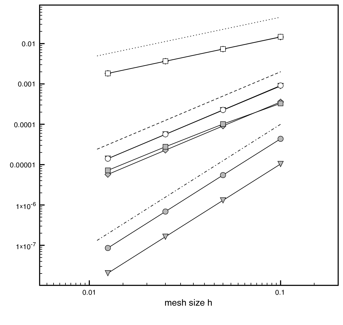
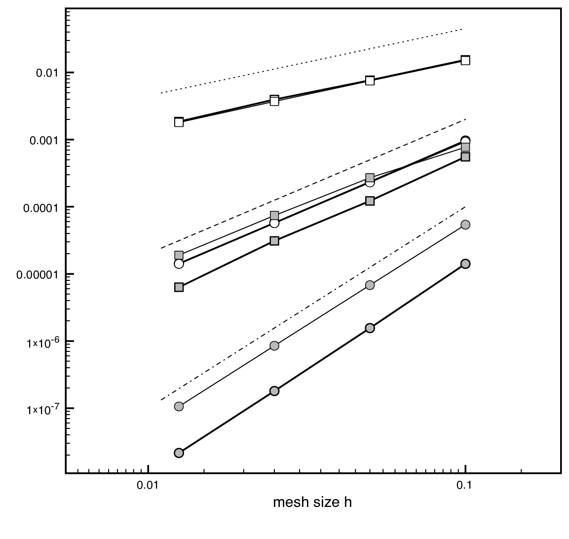
Here stands for functions continuous on each separate connected component of . It is straightforward to verify that the spaces are stable for our problem. In all figures below square markers refer to methods using and circles to methods using . Empty markers indicate convergence of the error in the -norm and filled markers in the -norm. We have also plotted for reference the slopes corresponding to convergence with in dotted line, in a dashed line and in dash dotted line. These reference plots are the same for all methods so that the relative performance can be assessed. In all cases the stabilisation parameter has been set to . This parameter appeared to give a resonable result for all methods. We observed that increasing the parameter can improve the accuracy in the multiplier at the expense of the primal variable and vice versa.
We consider the formulation (2.11\themathletter) with the stabilisation given by
and the finite element spaces proposed above. In figure 1\theletter, left plot, we give the convergence plots for and . Then we consider the method (4.17\themathletter) and give the same convergence curves in the right plot of (1\theletter). For comparison we also present the results obtained using the inf-sup stable finite element pairs . Finally we consider the penalty free version of Nitsche’s method, both the non-symmetric version given by equation (4.18\themathletter) and its symmetric equivalent that may be written
Observe that the stability properties of this latter method are unknown, but for the computations considered herein the method remained stable and optimally convergent. We report the convergence of the Nitsche type methods in the left plot of figure (2\theletter). The symmetric version is distinguished by thick lines. A consequence of the close relation between the Barbosa-Hughes method and Nitsche’s method is that in both the symmetric and the non-symmetric case the unpenalised Nitsche methods are recovered in the limit as the stabilisation goes to infinity. This is illustrated in the right plot of (2\theletter) where we show the variation -error of the difference between the solution obtained by the Barbosa-Hughes stabilisation and Nitsche’s method on a mesh as the penalty parameter goes to infinity. In both the non-symmetric and the symmetric case the penalty free Nitsche type methods are recovered. Observe the strong increase in the error for the symmetric case at approximately where the matrix becomes singular. For higher values of the penalty parameter no instabilities were observed.
We make the following observations. The -norm error is almost identical for all methods. For the -norm error all adjoint consistent methods have very similar error curves, whereas the lack of adjoint consistency is expressed only as a larger error constant and not in a loss of convergence order as expected from the analysis. In experiments not reported here we imposed Dirichlet conditions all around the domain to see the effects on the corners in the non-symmetric Nitsche method, but optimal convergence was still attained on the finest meshes. We also studied the error in the fluxes approximated by the multiplier and the results were similar to that of the -norm error.


VI. CONCLUSION
We have given an analysis of projection stabilised Lagrange
multipliers in an abstract framework and shown some applications of
this therory. We then showed how the residual based stabilisation
method of Barbosa-Hughes can be
interpreted as a method penalising the distance to a stable subspace
by relating it to the inf-sup stable penalty free Nitsche method. The
methods were tested and compared numerically on a simple model
problem. All these methods appear to have very similar properties. In
particular optimal convergence was observed in both the - and the
-norms independently of adjoint consistency. Nevertheless adjoint consistent
methods have smaller errors in -norm for a fixed mesh size and
similarly for the approximation of the fluxes. The observed difference was a moderate factor. One may
conclude from this that it is
reasonable that one may base the choice of method entirely on what is
the easiest to implement for a given application. It also follows from
the discussion of Section III. that the jump penalty operator
provides a stabilisation requiring minimal knowledge of the inf-sup
stable space .
Two open problems
are the question of stability of the penalty free symmetric Nitsche
method and accuracy in the -norm of the non-symmetric Nitsche
method.
Both of which are observed.
Acknowledgment
Section I. to III. of this paper was written for a doctoral course given in September 2009 at the doctoral school ICMS, Paris-Est Marne-la-Vallée, that I gave as invited Professor. The kind hospitality of Professors Alexandre Ern and Robert Eymard is graciously acknowledged. I also acknowledge funding from EPSRC (award number EP/J002313/1). Finally I would like to thank the reviewers of the paper whose constructive criticism helped improve the manuscript.
Appendix: construction of the Fortin interpolant
We will use the notation of section IV.B. and prove that the Fortin interpolant satisfying (2.5\themathletter) exists and that the stability constant is independent of how the interface cuts the mesh Note that the stability of the Fortin interpolant writes
where the hidden constant must be independent of the mesh-interface intersection. We introduce the extension operators such that for all , , and . Here denotes the mesh-domain defined as . Let denote an -stable interpolant. For each define the extended patch . Then on each patch define a function with , and
Define where
This construction is always possible, provided is a given (fixed) factor larger than , typically is sufficient.
Then the orthogonality condition of (2.5\themathletter) holds by construction. It remains to prove the -stability. By the triangle inequality and the disjoint supports of the we have,
| (6.1\themathletter) |
By the assumed stability of and we immediately have
For we consider one term in the sum and get by the construction
By the shape regularity of the there is no dependence on the mesh domain intersection in the constants. Summing over and using the fact that the are disjoint for fixed we obtain that
and the desired stability estimate follows by the approximation and stability properties of and the stability of . It remains to prove that
This follows by adding and subtracting in the left hand side, and using a triangle inequality to obtain
We now proceed using a global trace inequality, the stability of the interpolant and the above bound on the term , to show that
Collecting the above bounds concludes the proof.
References
References
- 1. I. Babuška. The finite element method with Lagrangian multipliers. Numer. Math., 20:179–192, 1972/73.
- 2. H. J. C. Barbosa and T. J. R. Hughes. The finite element method with Lagrange multipliers on the boundary: circumventing the Babuška-Brezzi condition. Comput. Methods Appl. Mech. Engrg., 85(1):109–128, 1991.
- 3. G. Barrenechea and F. Chouly. A local projection stabilized method for fictitious domains. Technical report, arXiv:1112.1592v1, 2011.
- 4. É. Béchet, N. Moës, and B. Wohlmuth. A stable Lagrange multiplier space for stiff interface conditions within the extended finite element method. Internat. J. Numer. Methods Engrg., 78(8):931–954, 2009.
- 5. R. Becker and M. Braack. A finite element pressure gradient stabilization for the Stokes equations based on local projections. Calcolo, 38(4):173–199, 2001.
- 6. R. Becker, E. Burman, and P. Hansbo. A hierarchical NXFEM for fictitious domain simulations. Internat. J. Numer. Methods Engrg., 86(4-5):549–559, 2011.
- 7. H. Ben Dhia and G. Rateau. Analyse mathématique de la méthode Arlequin mixte. C. R. Acad. Sci. Paris Sér. I Math., 332(7):649–654, 2001.
- 8. F. Brezzi. On the existence, uniqueness and approximation of saddle-point problems arising from Lagrangian multipliers. Rev. Française Automat. Informat. Recherche Opérationnelle Sér. Rouge, 8(R-2):129–151, 1974.
- 9. F. Brezzi and M. Fortin. Mixed and hybrid finite element methods volume 15 of Springer Series in Computational Mathematics. Springer-Verlag, New York, 1991.
- 10. F. Brezzi and M. Fortin. A minimal stabilisation procedure for mixed finite element methods. Numer. Math. 89 (2001), no. 3, 457–491.
- 11. E. Burman. Pressure projection stabilizations for Galerkin approximations of Stokes’ and Darcy’s problem. Numer. Methods Partial Differential Equations 24(1), 127–143, 2008.
- 12. E. Burman. A penalty free non-symmetric Nitsche type method for the weak imposition of boundary conditions. Technical report, arXiv:1106.5612, 2011.
- 13. E. Burman. Ghost penalty. C. R. Math. Acad. Sci. Paris, 348(21-22):1217–1220, 2010.
- 14. E. Burman and P. Hansbo. Fictitious domain finite element methods using cut elements: I. A stabilized Lagrange multiplier method. Comput. Methods Appl. Mech. Engrg., 199(41-44):2680–2686, 2010.
- 15. E. Burman and P. Hansbo. Interior-penalty-stabilized Lagrange multiplier methods for the finite-element solution of elliptic interface problems. IMA J. Numer. Anal., 30(3):870–885, 2010.
- 16. R. Codina and J. Baiges. Approximate imposition of boundary conditions in immersed boundary methods. Internat. J. Numer. Methods Engrg., 80(11):1379–1405, 2009.
- 17. C. R. Dohrmann and P. B. Bochev. A stabilized finite element method for the Stokes problem based on polynomial pressure projections. Internat. J. Numer. Methods Fluids, 46(2):183–201, 2004.
- 18. G. Dupire, J. P. Boufflet, M. Dambrine, and P. Villon. On the necessity of Nitsche term. Appl. Numer. Math., 60(9):888–902, 2010.
- 19. A. Ern ; J.-L. Guermond. Theory and practice of finite elements. Applied Mathematical Sciences, 159. Springer-Verlag, New York, 2004. xiv+524 pp. ISBN: 0-387-20574-8
- 20. F. Hecht, O. Pironneau, A. Le Hyaric, and K. Ohtsuka. FreeFem++ v. 2.11. User’s Manual. University of Paris 6.
- 21. A. Gerstenberger and W. A. Wall. An embedded Dirichlet formulation for 3D continua. Internat. J. Numer. Methods Engrg., 82(5):537–563, 2010.
- 22. M. Fortin. An analysis of the convergence of mixed finite element methods. RAIRO Anal. Numér. 11 (1977), no. 4, 341–354, iii.
- 23. V. Girault and R. Glowinski. Error analysis of a fictitious domain method applied to a Dirichlet problem. Japan J. Indust. Appl. Math., 12(3):487–514, 1995.
- 24. C. Grossmann. Penalties, Lagrange multipliers and Nitsche mortaring. Discuss. Math. Differ. Incl. Control Optim., 30(2):205–220, 2010.
- 25. A. Hansbo, P. Hansbo. A finite element method for the simulation of strong and weak discontinuities in solid mechanics. Comput. Methods Appl. Mech. Engrg. 193(33-35), 3523–3540, 2004.
- 26. P. Hansbo, C. Lovadina, I. Perugia and G. Sangalli. A Lagrange multiplier method for the finite element solution of elliptic interface problems using non-matching meshes. Numer. Math. 100 (2005), no. 1, 91–115.
- 27. M. Hautefeuille, A. Chandrasekhar, and J. E. Dolbow. Robust imposition of Dirichlet boundary conditions on embedded surfaces. Int. J. Numer. Meth. Engng, 2011. Published online.
- 28. P. Hild and Y. Renard. A stabilized Lagrange multiplier method for the finite element approximation of contact problems in elastostatics. Numer. Math., 115(1):101–129, 2010.
- 29. F. Liu and R. I. Borja. Stabilized low-order finite elements for frictional contact with the extended finite element method. Comput. Methods Appl. Mech. Engrg., 199(37-40):2456–2471, 2010.
- 30. J. Pitkäranta. Boundary subspaces for the finite element method with Lagrange multipliers. Numer. Math., 33(3):273–289, 1979.
- 31. J. Pitkäranta. Local stability conditions for the Babuška method of Lagrange multipliers. Math. Comp., 35(152):1113–1129, 1980.
- 32. G. Rapin and G. Lube. A stabilized scheme for the Lagrange multiplier method for advection-diffusion equations. Math. Models Methods Appl. Sci., 14(7):1035–1060, 2004.
- 33. R. Stenberg. On some techniques for approximating boundary conditions in the finite element method. J. Comput. Appl. Math., 63(1-3):139–148, 1995. International Symposium on Mathematical Modelling and Computational Methods Modelling 94 (Prague, 1994). \resetdefaults