Adaptive Network Coding for Scheduling Real-time Traffic with Hard Deadlines

We consider a time-slotted downlink system with one transmitter (e.g., base station) and $N$ receivers (users), as illustrated in Fig. 1. Time slots are synchronized across receivers and the transmission time of a packet corresponds to one time slot. The transmitter broadcasts $M$ packets to $N$ receivers over i.i.d. binary erasure channels with erasure probability $\epsilon$.¹¹ 1 The results derived in the paper can be readily applied to heterogeneous channels with different erasure probabilities. We assume immediate and perfect feedback available at the transmitter. For multimedia communications, it is standard to impose deadlines for delay-sensitive data (see, e.g., [15, 14, 4, 16, 17]). We assume that packets must be delivered to each receiver before $T$ slots, i.e., the deadline of each packet is $T$ slots. Any packet that cannot be delivered to all receivers by this deadline is dropped without contributing to the throughput.

Worth noting is that this model can be readily applied to finite-energy systems with NC, where the objective is to maximize the system throughput before the energy is depleted for further transmission. Therefore, the energy and delay constraints can be used interchangeably.

In Section III, we consider the basic model with one flow and one frame of $T$ slots. In Section IV, we generalize the model to multiple frames with multiple flows, where packets arrive at the beginning of each frame and they are dropped if they cannot be delivered to their receivers by the deadline of $T$ slots.

As noted above, the throughput gain of NC comes at the expense of longer decoding delay (since packets are coded and decoded as a block), which may reduce the throughput of the system due to the hard deadline constraints. Let $K$ denote the block size, i.e., the number of original packets encoded together by NC. We assume that the transmitter and each receiver know the set of coding coefficients, and the transmitter broadcasts the value of $K$ to receivers before the NC transmissions start. The coding coefficients can also be chosen randomly from a large field size (or from a predetermined coding coefficient matrix of rank $K$) such that with high probability $K$ packet transmissions deliver $K$ innovative packets in coded form to any receiver, i.e., the entire block of packets can be decoded after $K$ successful transmissions. As shown in [2], the probability that all receivers can decode the block of size $K$ within $T$ slots is given by

where $\binom{n}{m}$ denotes the number of combinations of size $m$ out of $n$ elements.²² 2 We can also employ random NC with a finite field size $q$. This would change the decoding probability (1) to a function of $q$. However, the general structure of the results will remain the same. Note that (1) strongly depends on the choice of block size $K$ and we can show that,

With block NC, there is the risk that none of the packets can be decoded by the receivers before the hard deadline. By using IDNC, it may be possible to start decoding without waiting for the entire block to arrive but the complexity of finding a suitable code may be overwhelming due to the dynamic programming involved in the problem [14]. Here, we provide the throughput guarantees for the worst-case scenario, where either the whole block or none of the packets can be decoded at any slot. There is a tradeoff between the block size and the risk of decoding. In particular, we cannot greedily increase $K$ to maximize the system throughput under the hard deadline constraints, since the risk that some receivers cannot decode the packets, i.e., $1-P(K,T)$, also increases with $K$ according to Lemma 2.1.

If the first block is delivered within the deadline, i.e., $T$ slots, the size of a new block (with new packets) needs to be re-adjusted for the remaining slots. In other words, we need real-time scheduling of network-coded transmissions depending on how close the deadline is. For example, when there is only one slot left before the deadline, the optimal block size is 1, since for any $K>1$, no receivers can decode the packets before the deadline. Also, the block size in a given slot statistically determines the remaining slots (before the deadline) along with the future system throughput. In Section III, we derive the optimal block size adaptation policy to maximize the system throughput under the deadline constraints for one frame with one flow. In Section IV, we generalize the results to the case with multiple frames with multiple flows.

The NC-based multimedia traffic scheduling of one frame is a sequential decision problem, which can be formulated as a Markov decision process (MDP) described as follows.

Horizon: The number of slots available before the deadline over which the transmitter (scheduler) decides the block size is the horizon. Due to the hard deadline, this MDP problem is a finite horizon problem with $T$ slots (one frame).

State: The remaining slots $t\in\{0,1,...,T\}$ before the hard deadline is defined as the state,³³ 3 We use the terms “state” and “slot” interchangeably. where $t=0$ denotes that there is no slot left for transmissions.

Action: Let $K_{t}$, $t\in\{1,...,T\}$, denote the action taken at state $t$, which is the block size for the remaining $t$ slots. Let $M_{t}$ denote the number of packets undelivered at state $t$. Thus, at state $t>0$, $K_{t}$ can be chosen from $1$ to $\min(t,M_{t})$. For $t=0$, the transmitter stops transmitting any packet, i.e., $K_{0}=0$. In general, the action space is defined as $\mathcal{K}_{t}=\{0,1,...,\min(t,M_{t})\}$.

Expected immediate reward: For the remaining $t$ slots, the expected immediate reward is the expected number of packets successfully decoded by all receivers, which is given by

where $P(K_{t},t)$ is given by (1), denoting the probability that each receiver can decode these $K_{t}$ packets within $t$ slots.

Block size adaptation policy: A block size adaptation policy $\mathcal{P}$ is a sequence of mappings, $\mathcal{P}=\{\mathcal{P}_{t}\}_{t=1}^{T}$, from $t$, $M_{t}$, $\epsilon$, and $N$ to an action $K_{t}\in\{0,1,...,\min(t,M_{t})\}$, i.e., $K_{t}=\mathcal{P}_{t}(t,M_{t},\epsilon,N)=\min(\mathcal{P}_{t}(t,\epsilon,N),M_{t})$. Without loss of generality, in Section III, we assume that $M_{t}$ is always larger than $t$, i.e., $K_{t}\in\{0,1,...,t\}$. This does not change the monotonicity structure of the block size with state $t$. We will discuss these structural properties in detail in Section III.

Total expected reward: Given the adaptation policy $\mathcal{P}$, the total expected reward for the remaining $t$ slots is given by

where the probability mass function $q_{t}(j)=P(K_{t},t-j)-P(K_{t},t-j-1)$ denotes the probability that the block of size $K_{t}$ is delivered over exactly $j$ slots before the deadline.

In each slot $t$, the optimal policy balances the immediate reward and the future reward by selecting a suitable block size $K_{t}^{*}$. In general, the approach of solving for the optimal block size by traditional dynamic programming [18] suffers from the “curse of dimensionality,” where the complexity of computing the optimal strategy grows exponentially with $t$. However, the optimal block size and its corresponding action space exhibit the monotonicity structures, and the optimal block size is bounded by the greedy block size. These unique structures make it possible to narrow down the search space of dynamic programming, and accordingly we develop a monotonicity-based backward induction algorithm (MBIA) with polynomial time complexity.

The MBIA searches for the optimal block size by backward induction and provides the optimal block size for each system state. Depending on the remaining time to deadline, the scheduler transmits coded packets with the optimal block size until each user receives enough packets to decode this block. Then, the scheduler adjusts the block size based on the current state, and proceeds with the new block transmission. This continues until the packet deadline expires or all packets are delivered. We present next the structural properties of block size adaptation problem that will lead to the formal definition of the MBIA.

Proof outline: As the number of remaining slots $t$ decreases, the maximum possible block size decreases as well, since $K_{t}\in\{0,1,...,t\}$; otherwise no receiver can decode the block of coded packets. $\square$

Proof outline: To show the unimodal property, it suffices to show that $R_{t}(K_{t})$ is log-concave, which can be shown by using induction method. The monotonicity property of $\hat{K}_{t}$ can be shown by invoking the contradiction argument and applying $\lim\nolimits_{t\rightarrow\infty}R_{t}(K_{t})=K_{t}$. $\square$

Fig. 2 shows the possible curves of $R_{t}(K_{t})$ for different values of $t$, illustrating the unimodal property of $R_{t}(K_{t})$ formally stated in Proposition 3.1. Based on Proposition 3.1, the monotonicity property of the optimal block size $K_{t}^{*}$ is given by the following theorem.

Proof outline: Based on Proposition 3.1, we can show that if $K_{t}^{*}<K_{t-1}^{*}$, $V_{t-1}(K_{t}^{*};\mathcal{P}^{*})>V_{t-1}(K_{t-1}^{*};\mathcal{P}^{*})$, which contradicts that $K_{t-1}^{*}$ is the optimal action in slot $t-1$. $\square$

As $t$ decreases, the risk that some receivers cannot decode the given block of packets increases for a fixed block size. Therefore, the scheduler becomes more conservative in the block size adaptation and selects a smaller block size.

Remarks: 1) For $t=1,2$, the optimal block size is $K_{t}^{*}=1$, which can be obtained by computing the Bellman equation (4). 2) When $N=1$, the optimal block size is $K_{t}^{*}=1$ for all $t$, since the plain retransmission policy with $K_{t}=1$ is better than the block coding with $K_{t}>1$ in the presence of the hard deadlines.

Proof outline: Based on Proposition 3.1, we can show if $K_{t}^{*}>\hat{K}_{t}$, along any sample path, the system throughput by taking the action $\hat{K}_{t}$ is at least as high as that by taking the action $K_{t}^{*}$, which contradicts that $K_{t}^{*}$ in this case is the optimal action in slot $t$. $\square$

Corollary 3.1 follows directly from Proposition 3.1 and Theorem 3.2. Based on these structural properties, we develop the MBIA, which is presented in Algorithm 1.

The MBIA confines the search space at state $t$ to the interval from $K_{t-1}^{*}$ (the optimal policy at state $t-1$) to $\hat{K}_{t}$ (the greedy policy at state $t$). Thus, the MBIA reduces the search space over time and reduces the complexity of dynamic programming as given by the following theorem.

Proof: Based on Proposition 3.1, $R_{t}(K_{t})$ has the unimodal property and therefore $\hat{K}_{t}$ can be solved efficiently by the Fibonacci search algorithm [19], which is a sequential line search algorithm with a complexity of $O(\log(t))$ at state $t$. Therefore, in each iteration, it takes $O(\log(t)+\hat{K}_{t}-K_{t-1}^{*})$ slots to find $K_{t}^{*}$. Based on Lemma 3.1, $\hat{K}_{t}-K_{t-1}^{*}$ is upper bounded by $t$. After some algebra, we show that the complexity of Algorithm 1 is bounded by $O(T^{2})$ and Theorem 3.3 follows. $\square$

Remarks: By using the MBIA, the optimal block size can be computed in polynomial time, which is a desirable property for online implementation. The optimal block size depends on the number of receivers and channel erasure probabilities. For different flows, the set of receivers may be different, which may result in different optimal block sizes, even when the number of remaining slots is the same across these flows. Therefore, without using the MBIA, offline schemes would need to compute the optimal policies for all possible receiver sets; however, this would be a computationally demanding task, as the number of receivers increases.

Based on the monotonicity properties of the greedy and optimal block sizes, the optimal policy becomes the plain retransmission, if the channel erasure probability is sufficiently large. This sufficiency condition for $K^{*}_{t}=1$ at slot $t$ is formally given as follows.

Proof outline: The proof follows directly by comparing $R_{t}(1)$ and $R_{t}(2)$ that are expressed as a function of $\epsilon$. $\square$

Note that (6) is a sufficient condition only and indicates the optimality of the greedy policy when $\epsilon$ is large enough.

Fig. 3 depicts how the threshold $\epsilon^{*}$ varies with $t$ and $N$. The underlying monotonicity property is formally stated in Corollary 3.2.

Remarks: 1) When the channel is good enough (with $\epsilon<\epsilon^{*}$), NC with $K_{t}>1$ can always improve the throughput compared to the plain retransmission policy. 2) As $t$ increases (i.e., the deadline becomes looser), the risk of decoding network-coded packets decreases, i.e., $\epsilon^{*}(t,N)$ increases. 3) As $N$ increases, it becomes more difficult to meet the deadline for each of $N$ receivers and therefore $\epsilon^{*}(t,N)$ drops accordingly.

The real-time scheduling policies presented so far focus on the expected throughput without considering the variation from the average performance. Therefore, it is possible that the instantaneous throughput drops far below the expected value. To reduce this risk, we use additional variation constraints to guarantee that the throughput performance remains close to the average. In particular, for each slot $t$, we introduce the variation constraint to the block size adaptation problem as follows:

where $\sigma_{t}^{2}$ is the maximum variation allowed in slot $t$ and the performance variation $v_{t}(K_{t})$ under action $K_{t}$ is given by

Since $v_{t}(K_{t})$ increases with $K_{t}$, (7) can be rewritten as the maximum block size constraint for each slot $t$, i.e.,

where $K_{t}^{\max}=\max\{K_{t}|K_{t}=\lfloor v_{t}^{-1}(\sigma_{t})\rfloor\}$, $v_{t}^{-1}(\cdot)$ is the inverse mapping of $v_{t}(\cdot)$, and $\lfloor x\rfloor$ denotes the largest integer smaller than $x$. The variation constraints do not change the monotonicity property of the optimal block size provided by Theorem 3.1. By introducing the variation constraints (9), the scheduler becomes more conservative in the block size adaptation. The additional bound $K_{t}^{\max}$ can be easily incorporated into the MBIA by changing the action space to $\mathcal{K}_{t}=\{K_{t-1}^{*},K_{t-1}^{*}+1,...,\min(K_{t}^{\max},\hat{K}_{t})\}$ at state $t$.

So far we have discussed the real-time scheduling policies with adaptive NC, where the channel erasure probability $\epsilon$ is perfectly known to the scheduler. The throughput performance of these policies depends on $\epsilon$; therefore, the scheduler needs to learn $\epsilon$ while adapting the block size, when it does not have (perfect) channel knowledge. Let $\hat{\epsilon}_{t}$ denote the estimate of the channel erasure probability in slot $t$. The scheduler can update $\hat{\epsilon}_{t}$ based on the feedback from the receivers. In slot $T$, if $\hat{\epsilon}_{T}<\epsilon$, we would expect with high probability that a block of packets with the size that is calculated with respect to $\hat{\epsilon}_{T}$ cannot be delivered before the deadline. Therefore, it is better to select the block size conservatively at the beginning, when the estimate $\hat{\epsilon}_{t}$ cannot be highly accurate yet, because of the small number of samples. As $\hat{\epsilon}_{t}$ improves over time, the block size can be gradually increased to improve the system throughput. Once the estimate is close enough to the actual value of $\epsilon$ after enough samples are collected, the block size should be adjusted (and reduced over time) according to the MBIA.

Clearly, there is a tradeoff between the channel learning and the block size adaptation. Here, we formulate a joint real-time scheduling and channel learning algorithm (Algorithm 2) to adapt the block size while updating the maximum likelihood estimate $\hat{\epsilon}_{t}$ of channel erasure probability. In slot $t$, based on the feedback, the scheduler can compute the packet loss ratio, $\epsilon_{t}=1-\frac{n_{t}}{N}$, where $n_{t}$ denotes the number of receivers that successfully receive a packet in slot $t$. Accordingly, the estimated channel erasure probability $\hat{\epsilon}_{t}$ is given by the moving average

The scheduler decides on the block size by comparing the temporal variation $|\hat{\epsilon}_{t}-\hat{\epsilon}_{t+1}|$ with a threshold $\delta$. A detailed description is given in Algorithm 2.

Remarks: Algorithm 2 captures the tradeoff between the channel learning and block size adaptation. There are two options for the scheduler depending on the relationship between $|\hat{\epsilon}_{t}-\hat{\epsilon}_{t+1}|$ and $\delta$. If the channel estimation is not yet good enough, Algorithm 2 chooses the block size conservatively by incrementing $K_{t}$ by at most $1$. Otherwise, Algorithm 2 computes the block size by applying the MBIA.

Fig. 4 illustrates for $N=5$ the monotonicity structure of the optimal block size (Theorem 3.1) and verifies that $K_{t}^{*}\leq\hat{K}_{t}$ (Theorem 3.2). Both the optimal and greedy block sizes increase when the channel conditions improve (from $\epsilon=0.5$ to $\epsilon=0.2$). Next, we evaluate the performance (average system throughput) of different policies. For comparison purposes, we also consider a soft delay-based conservative policy, where the scheduler chooses the largest block size with the expected completion time less than or equal to the number of remaining slots. The expected completion time is studied in [2], and it is given by

Fig. 5 compares the performance of the optimal, greedy, conservative and plain retransmission policies for $N=10$ and $T=10$. The plain retransmission policy always performs the worst, whereas the conservative policy performs worse than the greedy policy. However, as $\epsilon$ increases, all policies select smaller block sizes and their performance gap diminishes.

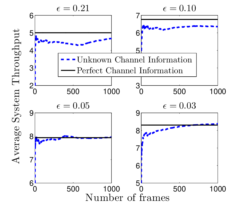
Fig. 6 shows the tradeoff between the average system throughput and the throughput variation. When the channels are good (e.g., $\epsilon=0.1$ in Fig. 6), the variation constraint (7) makes the scheduler choose a small block size, which reduces the average system throughput accordingly. However, there is no significant effect of (7) when channels are bad (e.g., $\epsilon=0.5$ in Fig. 6), since the scheduler already chooses a small block size for large $\epsilon$. Fig. 7 evaluates the performance of Algorithm 2 under channel uncertainty and show that Algorithm 2 is robust with respect to the variation of $\delta$ and achieves a reliable throughput performance close to the case with perfect channel information.

The scheduler allocates slots for each flow and uses the optimal real-time scheduling policy with adaptive NC developed in Section III to transmit network-coded packets. Given the arrivals, the scheduler needs to allocate a suitable number of slots for each flow to satisfy the delivery ratio requirement. This resource allocation is defined as a feasible schedule, $s=(s_{f})_{f\in\mathcal{F}}$, where $s_{f}$ denotes the number of slots allocated to flow $f$ and $\sum_{f\in\mathcal{F}}s_{f}\leq T$. Our goal is to maximize the weighted throughput subject to the delivery ratio and hard deadline constraints. We find the optimal schedule, i.e., the probability $Pr(s|a)$ that given the arrivals $a$, the schedule $s\in\mathcal{S}$ is used from the set $\mathcal{S}$ of all feasible schedules. Then, the expected service rate for flow $f$ is upper-bounded by

where $c_{f}(s_{f})$ is the expected number of packets that can be delivered under schedule $s_{f}$, which is a constant and can be solved by the MBIA. Hence, we formulate the joint resource allocation and block size adaptation as the following optimization problem:

where $w_{f}$ is the weight for flow $f$ and can be used as a fairness metric for resource allocation to each flow.⁶⁶ 6 The problem (13) can be generalized to the case with congestion control by treating the weights as virtual queues for flow rates (similar to the service deficit queues that we use later in Section IV-B). Note that (13) generalizes the problem studied in [21] by using adaptive NC schemes in packet transmissions.

Since (13) is strictly convex, the duality gap is zero from the Slater’s condition [20]. The dual problem is given by

where $\nu_{f}$ is the Lagrangian multiplier for flow $f$. The objective function of (14) is linear and the upper bounds for $\mu_{f}$ are affine functions. Therefore, the optimization problem (14) can be rewritten as:

Thus, we have the following gradient-based iterative algorithm to find the solution to the dual problem (14),

where $k$ is the step index, $\rho>0$ is a fixed step-size parameter, and $c_{f}(s_{f}^{*}(k))$ is the expected service rate for flow $f$ under schedule $s_{f}^{*}(k)$. Letting $\hat{\nu}_{f}(k)=\frac{\nu_{f}(k)}{\rho}$, (16) is rewritten as

Remarks: The update equation for $\hat{\nu}_{f}$ can be interpreted as a virtual queue for the long-term delivery ratio with the arrival rate $\lambda_{f}q_{f}$ and the service rate $\mu_{f}^{*}(k)$, which keeps track of the deficit in service for flow $f$ to achieve a delivery ratio greater than or equal to $q_{f}$. Note that (17) provides only the static solution to (14). Next, we provide an online scheduling algorithm which takes into account the dynamic arrivals of the flows.

The online scheduling algorithm is given by

where $\hat{c}_{f}(s_{f}^{*}(k))$ denotes the actual delivered number of packets under the schedule $s_{f}^{*}(k)$ depending on the channel realizations, and $\hat{a}_{f}(k)$ is a binomial random variable with parameters $a_{f}(k)$, the number of packet arrivals of flow $f$ in the $k$th frame, and $q_{f}$. This implementation for $\hat{a}_{f}(k)$ was proposed in [21]. At the beginning of each period, the schedule $s^{*}(k)$ is determined by (18). Then, the packets of each flow $f$ are transmitted with the MBIA in the scheduled $s^{*}_{f}(k)$ slots. The virtual queue $\hat{\nu}_{f}$ is updated based on the number of successfully delivered packets $\hat{c}_{f}(s_{f}^{*}(k))$ of each flow $f$. With Lyapunov optimization techniques [22, 23], it can be shown that (18) has the following properties.

The proofs follow from the optimization framework in [22, 23] and they are similar to the proofs presented in [21]. Note that the online scheduling algorithm (18) can approach within $O(\rho)$ of the optimal solution to (14) and does not require any knowledge of the packet arrival statistics.

We consider a network with two flows, each with five receivers. The packet traffic of each flow follows Bernoulli distribution with mean $\lambda_{f}$ packets/frame for $f=1,2$, and the length of each frame is $10$ slots. In the simulation, we set $\lambda_{f}=\lambda$ for $f=1,2$. The channel erasure probability $\epsilon$ is $0.3$, the weights $w_{f}$ are $1$ for all flows, the step-size $\rho$ is $0.1$, and the simulation time is $10^{5}$ frames.

We evaluate the performance of our algorithm by comparing the region of achievable rates $(\mu_{1},\mu_{2})$ with the plain retransmission under different traffic flow rates $\lambda$, where the achievable rates denote the feasible solution to (13) for given delivery ratio requirements $q_{f}$. By varying $q_{f}$, we find the achievable rate region. As illustrated in Fig. 8, the plain retransmission only achieves a small fraction of the region with adaptive NC. By using adaptive NC, the network can support flows with heavier traffic.

Fig. 9 shows the average service deficit $\hat{\nu}$ of two flows. The delivery ratio requirement of each flow is $0.8$. As $\lambda$ increases, $\hat{\nu}$ grows unbounded, which means that the conditions, $\mu_{f}^{*}>\lambda_{f}q_{f}$ for all $f\in\mathcal{F}$, are not satisfied, i.e., the arrival rates are not in the “stability” region, and the online scheduling algorithm cannot meet the delivery ratio requirements.

$P(K,T)$ is monotonically decreasing with $K$, if $\hat{P}(K,T)$ is monotonically decreases with $K$, where

such that $P(K,T)=(\hat{P}(K,T))^{N}$. First, we express

Since from (20) it follows that

is negative, $P(K,T)$ is monotonically decreasing with $K$.

1) To show that $R_{t}(K_{t})$ is unimodal, it suffices to show that $R_{t}(K_{t})$ is log-concave, i.e., $\hat{R}(K)=\frac{1}{N}\log(K)+\log(\hat{P}(K,T))$ is concave. Since $\frac{1}{N}\log(K)$ is concave, it suffices to show that for any given $T$, $\log(\hat{P}(K,T))$ is concave, i.e., $\hat{P}(K,T)$ is log-concave. Based on the definition of log-concavity, in what follows, we will show that

Based on (21), (22) can be rewritten as

We use induction to show (23). For $T=1,2$, it is obvious to see that (23) holds. For $T=3$, we can verify (23) by using (19). Assume that for $T=t>3$, (23) holds. For $T=t+1$, after some algebra, we have

which is based on the induction and (21).

2) Since $P(K_{t},t)$ is monotonically increasing with $t$ for any $K_{t}$, $R_{t}(K_{t})$ is monotonically increasing with $t$. Besides, as $t$ goes to infinite, $\lim\limits_{t\rightarrow\infty}R_{t}(K_{t})=K_{t}$, i.e., the block with length $K_{t}$ can be delivered almost surely. Therefore, for any $K<\hat{K}_{t}$, we can conclude that $R_{t+1}(\hat{K}_{t})>R_{t+1}(K)$. Since $\hat{K}_{t+1}$ is the optimal block size in slot $t+1$, i.e., $R_{t+1}(\hat{K}_{t+1})\geq R_{t+1}(\hat{K}_{t})$, if $\hat{K}_{t+1}<\hat{K}_{t}$, then we have $R_{t+1}(\hat{K}_{t+1})<R_{t+1}(\hat{K}_{t})$, which contradicts the fact that $\hat{K}_{t+1}$ is the optimal block size in slot $t+1$. Therefore, $\hat{K}_{t+1}\geq\hat{K}_{t}$.

The proof follows from a contradiction argument. Suppose that $K_{t}^{*}>K_{t+1}^{*}$. It can be shown that $K_{t}^{*}\leq\hat{K}_{t}$ by a contradiction argument. From Proposition 3.1, it follows that $R_{t}(K_{t}^{*})>R_{t}(K_{t+1}^{*})$ in slot $t$. Since $K_{t}^{*}$ is the optimal action in slot $t$, $V_{t}(K_{t}^{*};\mathcal{P}^{*})>V_{t}(K_{t+1}^{*};\mathcal{P}^{*})$. Since $K_{t}^{*}>K_{t+1}^{*}$ in slot $t$, when the optimal policy is applied, the future reward $J_{t}(K_{t}^{*})$ under $K_{t}^{*}$ is less than the future reward $J_{t}(K_{t+1}^{*})$ under $K_{t+1}^{*}$, due to the less remaining time under $K_{t}^{*}$. The future rewards under both actions are monotonically increasing with $t$, since $R_{t}(K)$ is monotonically increasing with $t$ for given $K$. Moreover, $\lim\limits_{t\rightarrow\infty}(J_{t}(K_{t}^{*})-J_{t}(K_{t+1}^{*}))=0$, since the probability of successfully delivering any given set of packets under any policy goes to 1, when the remaining time goes to infinity. This indicates that the gap between these future rewards decreases in slot $t+1$. Since $R_{t}(K)$ is monotonically increasing with $t$, we have $R_{t+1}(K_{t}^{*})>R_{t+1}(K_{t+1}^{*})$. Therefore, $R_{t+1}(K_{t}^{*})+J_{t+1}(K_{t}^{*})>R_{t+1}(K_{t+1}^{*})+J_{t+1}(K_{t+1}^{*})$, i.e., in slot $t+1$, the total expected reward under $K_{t+1}^{*}$ is less than that under $K_{t}^{*}$, which contradicts that $K_{t+1}^{*}$ is the optimal action in slot $t+1$.

The proof follows from a contradiction argument. Suppose that $K_{t}^{*}>\hat{K}_{t}$. For any sample path, the case with $\hat{K}_{t}$ will deliver the block earlier than the case with $K_{t}^{*}$. For the sample paths with the number of slots that all the channels between the transmitter and the receivers are good less than $K_{t}^{*}$, the reward under $\hat{K}_{t}$ is higher than that under $K_{t}^{*}$. For the other sample paths with the number of slots that all the channels between the transmitter and the receivers are good greater than $K_{t}^{*}$, the block with size $\hat{K}_{t}$ will be delivered earlier than that with size $K_{t}^{*}$. We assume that after the block with size $\hat{K}_{t}$ is delivered, the scheduler chooses to deliver the block with size 1, before the block with size $K_{t}^{*}$ is delivered. Then after the block with size $K_{t}^{*}$ is delivered, the optimal policy is applied for both cases. Obviously, in this case, both cases will generate the same reward. However, for the case with block size $\hat{K}_{t}$, the policy that we applied after the block with size $\hat{K}_{t}$ is delivered may not be optimal, which means that the reward under the optimal policy is no less than the reward of the policy we used. Therefore, the total expected reward under $K_{t}^{*}$ is less than that under $\hat{K}_{t}$, which contradicts the fact that $K_{t}^{*}$ is the optimal action in slot $t$.

References

- [1] R. Ahlswede, N. Cai, S. Li, and R. Yeung. Network information flow. IEEE Trans. Inform. Theory, 46(4):1204-1216, 2000.
- [2] A. Eryilmaz, A. Ozdaglar, M. Medard, and E. Ahmed. On the delay and throughput gains of coding in unreliable networks. IEEE Trans. Inform. Theory, 54(12):5511-5524, 2008.
- [3] J.-K. Sundararajan, D. Shah, and M. Medard. ARQ for network coding. In Proc. of IEEE ISIT, pages 1651-1655, 2008.
- [4] E. Drinea, C. Fragouli, and L. Keller. Delay with network coding and feedback. In Proc. of IEEE ISIT, pages 844-848, 2009.
- [5] Y. E. Sagduyu, and A. Ephremides. On broadcast stability of queue-based dynamic network coding over erasure channels. IEEE Trans. Inform. Theory, 55(12):5463-5478, 2009.
- [6] D. Nguyen, T. Tran, T. Nguyen, and B. Bose. Wireless broadcast using network coding. IEEE Trans. Veh. Technol., 58(2):914-925, 2009.
- [7] J. Barros, R. A. Costa, D. Munaretto, and J. Widmer. Effective delay control in online network coding. In Proc. of IEEE INFOCOM, pages 208-216, 2009.
- [8] T. Ho, R. Koetter, M. Medard, M. Effros, J. Shi, and D. Karger. A random linear network coding approach to multicast. IEEE Trans. Inform. Theory, 52(10):4413-4430, 2006.
- [9] D. Traskov, M. Medard, P. Sadeghi, and R. Koetter. Joint scheduling and instantaneously decodable network coding. In Proc. of IEEE Globecom Workshops, pages 1-6, 2009.
- [10] J. Heide, M. V. Pedersen, F. H. P. Fitzek, and T. Larsen. Network coding for mobile devices - systematic binary random rateless codes. In Proc. of IEEE ICC Workshops, pages 1-6, 2009.
- [11] W. Yeow, A. Hoang, and C. Tham. Minimizing delay for multicast-streaming in wireless networks with network coding. In Proc. of IEEE INFOCOM, pages 190-198, 2009.
- [12] A. A. Yazdi, S. Sorour, S. Valaee, and R. Y. Kim. Optimum network coding for delay sensitive applications in WiMAX unicast. In Proc. of IEEE INFOCOM, pages 2576-2580, 2009.
- [13] R. Li, and A. Eryilmaz. Scheduling for end-to-end deadline-constrained traffic with reliability requirements in multi-hop networks. In Proc. of IEEE INFOCOM, pages 3065-3073, 2011.
- [14] X. Li, C.-C. Wang, and X. Lin. On the capacity of immediately-decodable coding schemes for wireless stored-video broadcast with hard deadline constraints. IEEE J. Sel. Areas Commun., 29(5):1094-1105, 2011.
- [15] D. Nguyen and T. Nguyen. Network coding-based wireless media transmission using POMDP. In Packet Video Workshop, pages 1-9, 2009.
- [16] H. Gangammanavar and A. Eryilmaz. Dynamic coding and rate-control for serving deadline-constrained traffic over fading channels. In Proc. of IEEE ISIT, pages 1788-1792, 2010.
- [17] I.-H. Hou and P. R. Kumar. Scheduling heterogeneous real-time traffic over fading wireless channels. In Proc. of IEEE INFOCOM, pages 1-9, 2010.
- [18] D. P. Bertsekas, Dynamic Programming and Optimal Control, Athena Scentific, Belmount, Massachusetts, 2005.
- [19] J. Kiefer. Sequential minimax search for a maximum. Proc. Amer. Math. Soc., 4(3):502-506, 1953.
- [20] S. Boyd and L. Vandenberghe. Convex Optimization. Cambridge, U.K.: Cambridge Univ. Press, 2004.
- [21] J. J. Jaramillo, R. Srikant, and L. Ying. Scheduling for optimal rate allocation in ad hoc networks with heterogeneous delay constraints. IEEE J. Sel. Areas Commun., 29(5):979-987, 2011.
- [22] L. Georgiadis, M. J. Neely, and L. Tassiulas. Resource allocation and cross-layer control in wireless networks. Foundations and Trends in Networking, 1(1):1-149, 2006.
- [23] M. J. Neely. Stochastic network optimization with application to communication and queueing systems. Synthesis Lectures on Communication Networks, 3(1):1-211, 2010.
- [24] J. Yackoski, B. Azimi-Sadjadi, A. Namazi, J. H. Li, Y. E. Sagduyu, and R. Levy. RF-NEST: radio frequency network emulator simulator tool. In Proc. of IEEE MILCOM, pages 1882-1887, 2011.
- [25] J. Ahrenholz, C. Danilov, T. Henderson, and J. Kim. CORE: a real-time network emulator. In Proc. of IEEE MILCOM, pages 1-7, 2008.