Driven Brownian coagulation of polymers
Abstract
We present an analysis of the mean-field kinetics of Brownian coagulation of droplets and polymers driven by input of monomers which aims to characterize the long time behavior of the cluster size distribution as a function of the inverse fractal dimension, , of the aggregates. We find that two types of long time behavior are possible. For the size distribution reaches a stationary state with a power law distribution of cluster sizes having exponent . The amplitude of this stationary state is determined exactly as a function of . For , the cluster size distribution never reaches a stationary state. Instead a bimodal distribution is formed in which a narrow population of small clusters near the monomer scale is separated by a gap (where the cluster size distribution is effectively zero) from a population of large clusters which continue to grow for all time by absorbing small clusters. The marginal case, , is difficult to analyze definitively, but we argue that the cluster size distribution becomes stationary and there is a logarithmic correction to the algebraic tail.
pacs
82.20.-w,82.35.Lr,83.80.JxI Introduction
Aggregation underlies numerous phenomena from milk curdling and blood coagulation to planet and star formation. A review of the earlier work on aggregation has been given by Chandrasekhar [1]; the following work is summarized in a number of books and reviews [2, 3, 4, 5, 6, 7, 8]. This research field has been initiated by a pioneering work of Smoluchowski [9] who established the framework for the analysis of aggregation. Smoluchowski considered well-mixed diluted systems and argued that the governing equation for the concentration of clusters of “mass” (that is, clusters composed of monomers, where the monomers are the clusters of the minimal mass) reads
| (1) |
Here is the rate at which clusters of mass and merge. Only binary collisions are taken into account since the system is assumed to be diluted. Mathematically, the reaction rates form an infinite symmetric matrix, ; the pre-factor in front of the gain terms on the right-hand side of (1) is needed to avoid double counting.
In addition to devising the mathematical framework underlying aggregation processes, Smoluchowski also computed the reaction rate in the most important case of Brownian coagulation. Namely, assuming that aggregates are spherical, Smoluchowski showed that
| (2) |
where and are the diffusion coefficient and the radius of the cluster of mass . Invoking the Stokes-Einstein relation between the diffusivity of a spherical (three-dimensional) object and its radius yields and hence Eq. (2) gives . Using additionally volume conservation, , one arrives (up to a multiplicative factor that can be absorbed into the time variable) at the following expression for the Brownian reaction rate
| (3) |
Rate equations (1) with the Brownian reaction rates (3) have never been solved. It is not shocking, of course, as mathematically they form an infinite set of coupled non-linear differential equations (1) with varying coefficients (3). For simpler reaction rates, Eqs. (1) can admit analytical solutions. For instance, Smoluchowski already noticed [9] that the Brownian reaction rate is homogeneous, . This feature suggests to consider the simplest such reaction rate, const. In this situation the rate equations (1) are indeed solvable [9, 1]. A very few other solvable cases have been found in later work (see [3, 6, 7, 8] for review), yet for all these years there has been no progress for the Brownian reaction rate. This classical case appears as analytically intractable problem as it originally looked.
In this work, we consider aggregation with input. Such driven aggregating systems often approach a non-equilibrium steady state [10, 11, 12] and the steady states tend to be more tractable. The details of input play rather limited role, e.g. they do not affect the emerging large mass behavior, if only clusters of small mass are injected. It is customary to assume that only monomers are injected. The governing equations then read
| (4) |
where we set the strength of the monomer flux to unity. (The flux strength can always be absorbed into the time variable.)
In the long time limit, the mass distribution can become stationary. In this situation one must solve
| (5) |
The stationary solutions, when they exist, often exhibit power-law behavior. These are non-equilibrium stationary states which arise due to the flux of mass from small mass scales to large mass scales supplemented by input at the small mass scale. These states are analogous to the flux-dominated stationary states that occur in fluid turbulence [13], passive scalar advection [14], wave turbulence [15], granular gases [16], and other driven aggregation systems [17, 18, 19, 20, 21].
In this paper we present a detailed analysis of the long-time behavior of the cluster size distribution for range of physically relevant models of Brownian coagulation with input of monomers which are parameterized by a single scaling exponent, , which is related to the fractal dimension of the aggregates. We start by describing the parameter space of relevant models in Sec. II and outline where problems of Brownian coagulation fit in this space. Next in Sec. III we study the cases which includes Smoluchowski’s original problem of Brownian coagulation of spherical droplets. We show that, in this regime, the size distribution becomes stationary for large times. For the case of spherical droplets, we show that the tail of the size distribution has the form
| (6) |
in the limit, the first exact result for this classical problem to best of our knowledge. In Sec. IV we study the cases where we find that the size distribution does not become stationary and characterize the dynamics for such kernels which include the physically interesting cases of stiff polymers () and polymers in an ideal solvent (). Finally in Sec. V, we provide some insights into the marginal case of an ideal polymer, although a complete analysis eludes us. We close with a short discussion.
II Models of Brownian coagulation
Before beginning our study Brownian coagulation of polymers, let us first briefly describe the wider parameter space of models in which Brownian coagulation sits. This will help to place our subsequent work in context.
II.1 A two-parameter class of reaction rates
The two-parameter class of homogeneous reaction rates given by
| (7) |
has been extensively studied (mostly without input) in the literature. See [7] for a review. The reason is that members of this class, for different values of the parameters and , reproduce various rates (or their asymptotics) that appear in applications.
We shall only discuss models for which the exponents and satisfy
| (8) |
The reason is that a system with kernel (7) undergoes a gelation transition when . Gelation corresponds to a loss of mass conservation in Eq. (1) after a finite time [22]. In the absence of a source of monomers, a gelling system reaches a steady state, but the steady state is trivial, namely the entire system is comprised of a single cluster which, in the limit of an infinite system, has infinite size. (In the presence of a source, a stationary state can be reached for such gelling systems [20] but they contain only finite total mass which considerably complicates the question of how the stationary state is approached dynamically. In particular, the scaling analysis outlined in the appendix fails since the first moment of the scaling function diverges.)
In addition, following the majority of work in this field, we shall further restrict the possible values of the parameters and to the range
| (9) |
The mathematical reason is that when , and/or , the system exhibits a highly singular phenomenon known as instantaneous gelation (see [8]). This essentially means that the solution of the infinite set of rate equations is ill-defined. One can make sense of a regularized version of Eq. (1) in this regime but the cut-off plays a crucial role [23]. In any case, for systems where coagulation requires physical contact between clusters, the reaction rate cannot grow faster than the masses of the clusters. The requirements (9) are then natural in such cases.
It is instructive to recall the derivation [12] of the stationary state for the rates (7), modulo the restrictions on the values of and discussed above. We shall employ the generating function approach [24]. We denote generating functions by
| (10) |
and the corresponding moments by
| (11) |
To find a stationary solution to (4), (7) we multiply (4) by and sum over to obtain
| (12) |
Let us assume that the cluster size distribution decays algebraically for small cluster sizes. Various exact solutions for particular kernels and the scaling argument outlined in Appendix A suggest that algebraic decay is plausible:
| (13) |
To determine the decay exponent and the amplitude let us recast the conjectural asymptotic behavior of the mass distribution into a singular behavior of the generating function. Indeed, the algebraic large behavior (13) of is equivalent to the following singular behavior of the generating functions in the limit:
| (14a) | ||||
| (14b) | ||||
Substituting expansions (14a)–(14b) into equation (12) and matching the constant terms we obtain . Matching then the leading behaviors we recover known results [12] for the decay exponent
| (15) |
An expression for the amplitude is rather cumbersome, but using standard identities for the Euler’s Gamma function it simplifies to
| (16) |

Using Eqs. (15)–(16) we can determine when the system can reach a steady state. First, we must assure that the series constituting and are convergent. This implies that and , which in conjunction with (15) lead to
| (17) |
This requirement simultaneously guarantees that the expression (16) for the amplitude is acceptable. The validity of (17) and (8) actually ensures the validity of (9). Geometrically the region in the plane where (17) and (8) are satisfied, and thus a steady state is reached, is the semi-infinite strip denoted in Fig. 1 by region A.
It is possible that the steady state is never reached. The analysis above shows that this can happen only outside the semi-infinite strip denoted by region C in Fig. 1. For instance, a sub-monolayer epitaxial growth is described by the generalized sum-kernel reaction rates
| (18) |
These rates are included in the class of rates (7) if one sets and . Two physically interesting cases are (this occurs when ad-atoms undergo “terrace” hopping) or (for the “periphery” hopping mechanism) [25]. In both of these cases, and generally when , the system evolves ad infinitum [18, 19], e.g. the cluster density grows as for . In the borderline case of , there appears an additional nested logarithm [18, 19], viz. the cluster density increases as . These behaviors are difficult to confirm by solving numerically mean-field rate equations, let alone to observe in simulations of a sub-monolayer epitaxial growth [26].
II.2 Brownian coagulation of polymers
Let us now restrict our attention to the main topic of this paper, the rates for Brownian coagulation. The generalization of the Smoluchowski formula, (2), from three to dimensions is . In the physically interesting two- and three-dimensional settings, the range of relevant models is rather limited.
If aggregation occurs on a two-dimensional substrate 11 1 More precisely, the factor in Smoluchowski formula should be replaced by in 2D; here we ignore this slowly varying logarithmic factor., then . Now the diffusion coefficient often varies algebraically with the size of the cluster, with being the mobility exponent, and this leads to the kernel (18); the corresponding behaviors have been investigated in Refs. [18, *KMR1999].
In three dimensions for spherical aggregates we arrive at (3). For fractal aggregates one would get a generalized Brownian kernel
| (19) |
where is the inverse fractal dimension of clusters. Most of the rest of this paper is devoted to the study of the solutions of Eq. (1) with these rates as the parameter is varied. The only difference between Eq. (19) and Eq. (7) with is an additional constant factor in (19) which actually affects the steady state. The analysis, however, is similar as we shall see in the next section. If we ignore this additional factor of 2 for the moment, the amplitude given by (31) remains positive as long as . Since is the fractal dimension of clusters, we conclude that the Brownian coagulation with input in three dimensions results in a stationary mass distribution if . The amplitude vanishes when thereby questioning that the mass distribution reaches a stationary limit in this case. Physically is realized when clusters are membranes.
A range of interesting behaviors arises when clusters are polymers. Coagulation often generates polymers. For instance, this naturally occurs if monomers have two reactive bonds. Schematically we can represent a monomer as . Pairs of monomers collide to create dimers with two reactive bonds, and generally clusters are polymers with two reactive bonds: . In polymer physics, we encounter three typical situations [28]. For the ideal chain, equivalently a polymer in the so-called solvent, the polymer is essentially a random walk, so , or . For a polymer in a good solvent, . Based on the discussion above, we expect that the mass distribution in this case does not reach a steady state 22 2 For the polymer in bad solvent, and we recover the classical Brownian coagulation kernel (3).. The same is true when polymers are very stiff, so that the kernel is given by (19) with .
In the following sections we address the challenge of understanding driven Brownian coagulation, as characterized by the Brownian kernel (19), in the range of the parameter space indicated by the solid line in Fig. 1. The previous discussion suggests that the cases , , and are physically most interesting. We first study the stationary case, in Sec. III. We then study the non-stationary case, , in Sec. IV. We leave the marginal case, , to the final Sec. V since it is the most challenging.
II.3 Remarks on numerical simulations

All numerical simulations presented in this paper were done using a variant of the coarse-graining method described in Refs. [30, 31]. Numerically, one must necessarily truncate Eq. (1) at some large cluster size which we denote throughout by . The choice of truncation is not unique. We chose to truncate by requiring that all clusters having mass greater than are removed from the system. For all dynamical simulations, care was taken to ensure that simulations were halted before the cluster size distribution started to feel the presence of this cut-off. We validated the code by comparing the amplitude of the stationary state against the exact result, Eq. (16). The results are shown in Fig. 2 for the kernel (7) with . We can see that, our numerical measurements are in exact agreement for small values of . As approaches , however, there is a considerable finite size effect which diminishes as the cut-off, , is increased.
III Stationary case:
III.1 Constant kernel
We begin with the simplest case when the merging rate is constant, . In this setting one can determine both the steady state mass distribution and several temporal characteristics. (This has been done e.g. [10, 11] and reviewed in [7, 8].) Hence this model sheds the light on the emergence of the steady state. Without loss of generality, we set in Eqs. (20). This choice can be achieved by appropriate rescaling of the density and time. The rate equations for the aggregation process that proceeds with a constant merging rate and driven by input of monomers then read
| (20) |
The total density of clusters, , is just the zeroth moment of the cluster size distribution. Summing Eqs. (20) we find that satisfies
| (21) |
so for an initially empty system
| (22) |
Plugging (22) into the first rate equation (20) we obtain , from which the density of monomers is
| (23) |
Generally, one can solve Eqs. (20) recursively to give
| (24) |
This formal solution quickly gets very unwieldy. Equations (22)–(23) show that the system reaches a non-trivial steady state 33 3 We are mostly interested in the steady state, so to make formulas less cluttered we write instead of ., . See Fig. 3.
The determination of from the time-dependent solution, (24) is impractical. A simpler procedure is based on the generating function technique introduced in Sec. II.1. We multiply Eq.(20) by , sum over and set the left-hand side to zero to obtain a stationary state. This transforms the infinite system (20) into a quadratic equation for the generating function :
Solving this equation we get . Expanding we arrive at
| (25) |
Note that for large , so that the mass density diverges. This is not surprising since
| (26) |
due to mass conservation.
When is large, the mass distribution is very close to stationary for sufficiently small masses , while for the mass distribution is essentially zero. The crossover mass is found from
| (27) |
implying that . The scaling analysis and numerical measurements presented in Appendix A suggest that is true for all values of in the range .
III.2 Brownian coagulation with input

Consider steady states in a class of models with the generalized Brownian kernel (19). Adopting the notation of Eqs. (10) and (11), multiplying (4) by and summing over , we arrive at the following equation for the generating functions
| (28) | |||||
Expanding , and in the limit
| (29) |
and substituting (29) into Eq. (28) we obtain in the zeroth order 44 4 Thus we cannot determine the steady state cluster density . The same holds for models considered in Sect. II.1.. Matching the leading terms in in this expansion, we determine the decay exponent to be and obtain a relation for the amplitude :
| (30) |
From this we obtain
| (31) |
For the classical Brownian coagulation () we arrive at the announced prediction (6) for the tail. Note that if one ignores the constant in (3), then the factor in (6) would be replaced by 55 5 This follows from (16) with .. The scaling functions (see Eq. (65)) for the constant kernel case, , and the Brownian coagulation case, , are plotted in Fig. 4 multiplied by a factor of . The plateaux for small masses indicate that the scaling exponent is very well supported numerically. Furthermore the predicted values for the amplitudes of these plateaux are in reasonable agreement. The discrepancy for the case can be traced to a finite size effect. It is interesting to observe that the large mass structure of the size distribution is not trivial with a characteristic “bump” being clearly visible. We remark that a somewhat similar bump is observed hydrodynamic turbulence as the energy cascade enters the dissipation range. In that context, this bump is known as the “bottleneck effect” [35] and can be attributed to the depletion of nonlinear interactions due to the decay of the energy spectrum as it enters the dissipation range. It is tempting to suggest, by analogy, that the bump in Fig. 4 is the result of the depletion of the reaction rate for large masses due to the absence of potential coagulation partners ahead of the front. Further investigation would be required to test this suggestion quantitatively. In any case, this bump is typical for all values of and plays a very important role in the following section where we analyze the case of .
IV Nonstationary case
IV.1 Stiff Polymers ()


The Brownian coagulation of stiff polymers is described by reaction rates
| (32) |
Let us first explicitly demonstrate that the stationary state is never reached. For the kernel (32), the first few governing equations (4) read
| (33) |
where we have taken into account mass conservation (26) and again adopted the notation (11) to denote moments of the cluster size distribution.
In the long time limit and therefore from (33) we find the leading asymptotic behavior of the densities of light clusters:
These partial results reveal the general pattern, viz.
| (34) |
Thus for any fixed mass, the corresponding density approaches to zero: . The formulas (34) are applicable before the minimum is reached.
Plugging (34) into the governing equations one finds that the amplitudes are determined by recurrence ,
| (35) |
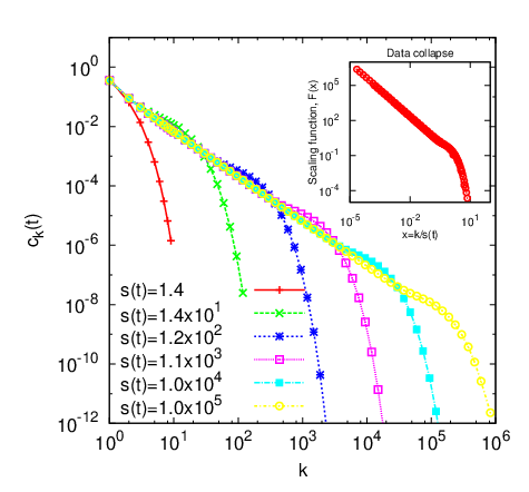
The sequence , etc. does not appear in 66 6 Online Encyclopedia of Integer Sequences, http://oeis.org and apparently does not admit a compact expression that depends only on . The asymptotic behavior of the amplitudes is simple. We need only one relation, when , which immediately follows from (35) and (32). Using this together with (34) one finds that for a fixed large , the mass distribution quickly decreases with when , a minimum is reached at , and then starts to increase. Fig. 5 shows the time evolution of the cluster distribution for stiff polymers obtained from numerical simulations. The emergence of a minimum is clearly observed. The predicted linear increase in the position of the minimum is well supported by numerics (main panel of Fig. 6). The predicted exponential decrease of with time is also well supported by numerics (inset of Fig. 6) although the rate of decrease seems to be less than 2.
The behavior of the mass distribution in the region is harder to understand than the behavior (34) in the ‘boundary layer’ region . Before analyzing the mass distribution in the region let us look at some higher order moments which encode a lot of information about the mass distribution. Generally, the moments evolve according to rate equations
| (36) |
etc. Specializing (36) to the reaction rate (32) gives
| (37) |

We have analyzed equations (37) using some guess work guided by simulations. The emerging behavior is quite simple. The asymptotic of the moment , and more generally any moment with , is dominated by monomers. In particular, the moment which appears in Eqs. (37), is given by
| (38) |
in the leading order (see red crosses in Fig. 7). The moments with exhibit a simple scaling behavior:
| (39) |
We have since . To find other amplitudes we insert (39) into (37) and obtain
etc., from which
| (40) |
Generally all with can be expressed through which therefore remains the sole unknown amplitude. Numerics (see inset of Fig. 7) indicate that . These relationships between moments are verified numerically for the first few moments (the main panel of Fig. 7).
The asymptotic behaviors (38)–(39) tell us that the mass distribution exhibits a scaling behavior outside the boundary layer region. If is the typical mass scale and is the typical density scale, the moments will exhibit the scaling behavior
| (41) |
The consistency between (39) and (41) sets
| (42) |
The same mass scale characterizes the Brownian coagulation in the situations when the mass distribution approaches a stationary limit, namely for the reaction rate (19) with . In this case, when , and the same argument as in (27) gives . The time evolution of the cluster size distribution is shown in Fig. 5 and clearly illustrates the predicted separation of the size distribution into two populations of clusters: a boundary layer near the monomer scale and a broader distribution of large clusters. The inset of Fig. 5 demonstrates that the large mass part of the cluster distribution collapses very well when rescaled using the theoretical scaling given by Eq. (42).
In addition to the scaling contribution to the moment , there is a contribution coming from the boundary layer region where the mass distribution follows (34). Actually the contribution from the boundary layer region is dominated by monomers. The scaling contribution to the moments dominates when and the monomer contribution dominates when ; at the marginal case of both contributions are comparable. These arguments explain (38), and more generally when , and (39) for .
Using the scaling form of the mass distribution
| (43) |
we can express the amplitudes via the integer moments of the scales mass distribution
| (44a) | ||||
| (44b) | ||||
| (44c) | ||||
Let us now try to determine the scaled mass distribution . When , the reaction rate (32) becomes and therefore the gain term in the Smoluchowski equation (4) can be re-written as
| (45) |
while the loss term simplifies to
| (46) |
The sum on the right-hand side of Eq. (45) contains the summation over the boundary layer and scaling region. The former is dominated by the contribution from monomers, while in the scaling region the summation can be replaced by integration. Therefore
| (47) |
Inserting Eqs. (45)–(47) into (4) gives
where we have also used . We now replace the difference by the derivative and use the scaling form (43) to find the governing equation for the scaled mass distribution
| (48) |
where, as in Eq. (40), we used notation . We must solve (48) subject to
| (49) |
It seems impossible to find an analytic solution of the boundary-value problem (48)–(49). However, we can determine the asymptotic behaviors and the qualitative shape of the scaled mass distribution. For instance, in the small limit keeping the dominant terms simplifies (48) to , from which
| (50) |
In the opposite limit, the scaled mass distribution decays exponentially
| (51) |
Plugging (51) into (48) and taking the limit we arrive at an equation that determines the amplitude :
Overall, the scaled mass distribution has a bell-shaped curve which vanishes exponentially fast in the and limits.
Note that without input the scaled mass distribution also has a bell-shaped curve and similar asymptotic behaviors [37], though the mass scale is different, , and the scaling ansatz is given by instead of (43). The most important distinction from the driven case is the lack of the boundary layer region.
IV.2 Polymers in Good Solvents:

The physically interesting situation of polymers in good solvents corresponds to , but the following analysis applies to the entire region . The procedure is essentially the same as for the case. The densities of monomers and dimers satisfy
| (52) |
Therefore asymptotically we have for monomers, for dimers, and generally
| (53) |
where the amplitudes are determined by recurrence and (35). The mass distribution is described by Eqs. (53) in the boundary layer region.
The first few integer moments satisfy
| (54) |
From these equations we see again the validity of the scaling behavior (39) which implies Eqs. (42)–(43). Using (39) with we conclude that and therefore
| (55) |
The same arguments as in Sec. IV.1 show that the monomers provide the dominant contribution to the total cluster density . Thus asymptotically
| (56) |
These scaling laws are verified numerically in Fig. 8. We remark that there is again a very strong finite size effect as approaches the marginal value of so that for the physically interesting case of we were unable to integrate for times long enough to observe the final asymptotic scaling predicted by (56) although the trend is clearly evident from the behavior of the larger values of .
V Marginal case of ideal polymer chains:

When , the amplitude given by Eq. (31) vanishes indicating that our analysis does not apply to this situation. The approach that has led to Eq. (31) is based on two assumptions: The emergence of a stationary solution and an algebraic behavior (13) of the stationary solution. Obviously, at least one of these assumptions is incorrect when . In this marginal case the major assumption regarding stationarity appears to work, while the secondary assumption of the power-law behavior (13) no longer holds. Since the power-law asymptotic is valid for all , one anticipates that the deviation is merely logarithmic. This suggests the conjectural asymptotic
| (57) |
There are some parallels with a problem in wave turbulence which we studied previously [38]. In the turbulence setting, the corresponding expression for the amplitude diverges rather than vanishes for a particular marginal kernel, and we did find that this divergence led to a logarithmic correction. The current problem seems to be considerably more difficult as our final asymptotic (62) involves a product over repeated logarithms.
Before proceeding we note that the assumption that the cluster densities become stationary in the limit tells us that the moment
| (58) |
must remain finite. Indeed, the rate equation for the monomers
tells us that the moments , and must remain finite (of course, the finiteness of the moment suffices) and the stationary value for the monomer density is given by
| (59) |
The conjectural behavior (57) of the tail is compatible with the finiteness of the moment when . Since we do not know a-priori that the cluster size distribution becomes stationary, we check the finiteness of the moments for large times numerically (see inset of Fig. 9) and find fairly strong evidence that the relevant moments tend to finite limits as in support of the assumption of stationarity. The stationary value of the monomer density is well described by Eq. (59) as shown in the main panel of Fig. 9.


To determine the exponent we use again the generating function approach and arrive at (28). The conjectural behavior (57) leads to certain behaviors of the generating functions in the limit, yet the results are inconsistent for all . For , the results are almost consistent, namely after canceling the dominant terms one eventually arrives at a relation of the form . Formally, this is of course inconsistent, although the error is much smaller than for any . Another drawback is that for the moment diverges, although in a very mild logarithmic manner.
Thus we should take , although the ansatz (57) with this is still slightly incorrect. A similar prediction is obtained by entirely different means in Appendix B. After a bit of trial and error one arrives at an improved ansatz
| (60) |
The finiteness of the moment now implies . The singularity analysis of the generating function equation (28) shows that results are inconsistent for all , while for the inconsistency is the weakest, namely one gets . (We use notation for the repeated logarithm: By definition and .) Thus we should take , although the ansatz (60) with this is still slightly incorrect. Trying
| (61) |
one again finds that and the ansatz (61) should be correct by another multiplicative factor , and then by , etc. In other words
| (62) |
A similar subtle behavior characterized by an infinite product of repeated logarithms arises in reversible polymerization [39]. In practice, the repeated logarithms are essentially undetectable, so at best one can hope to see
| (63) |
These predictions are compared with numerics in Fig. 10. Figure 10(A) shows the time evolution of the cluster size distribution for the marginal case . The same data are shown in Fig. 10(B) multiplied by a factor of . The fact that the tail of the size distribution now looks almost flat on this plot indicates that the exponent is correct although there is still some weak variation with in the tail which may indicate a logarithmic correction. The inset of Fig. 10(B) shows the same data collapsed according to the scaling (42). It is clear that, similar to what we found for the non-stationary case in Sec. IV.1, the leading bump of the size distribution is very well described by scaling whereas the tail is not. Figure 10(C) shows the same data multiplied by an additional factor of as suggested by the theoretical arguments outlined above. We concede that it is open to interpretation whether the result demonstrates a more convincing plateau for small cluster sizes than the corresponding data without the logarithmic correction plotted in Fig. 10(B). It seems that the honest conclusion to draw is that the numerics are unable to give definitive support to the conjectured behavior (63) although the fact that we obtained the same answer by completely different means in Appendix B gives us some degree of confidence that we have obtained the correct asymptotic behavior.
VI Conclusions and discussion
To conclude we have presented an extensive analysis of the kinetics of Brownian coagulation of polymers in the presence of a source of monomers at the mean field level. Our study focused on the determining the structure of the cluster size distribution for large times as a function of the exponent , the inverse fractal dimension of the polymer aggregates. We find that this behavior falls into two classes, depending on the value of .
If the exponent of the kernel is in the range then the size distribution for any fixed mass becomes stationary for large times (although the typical mass continues to grow as for all times). The resulting stationary state is a non-equilibrium stationary state characterized by a balance between the generation of new clusters by the injection and subsequent aggregation of monomers and the loss of clusters via aggregation. The stationary state carries a flux of mass through the space of cluster sizes from small clusters to large. We determined that the scaling exponent of this stationary state is always and obtained an exact expression for the amplitude of this stationary state as a function of . During the course of this analysis, we analytically determined the stationary cluster size distribution in the presence of source of monomers for the problem of Brownian coagulation of spherical droplets () originally introduced by Smoluchowski at the foundation of this field almost one century ago.
If the exponent is in the range , which includes the physically relevant cases of stiff polymers and polymers in an ideal solvent we find that the cluster size distribution never reaches a stationary state. Rather the population of clusters splits into two populations resulting in a bimodal cluster size distribution. In this regime, the size distribution exhibits a narrow “boundary layer” of clusters near the monomer scale. This boundary layer is separated by a gap, in which the cluster size distribution goes exponentially to zero in time, from a population of large clusters which continue to grow for all times by absorbing small clusters.
The marginal case, corresponding to ideal polymers, turned out to be very difficult to understand theoretically since it exhibits aspects of both behaviors. Our analysis suggests that the size distribution in this case does become stationary, but the tail acquires a logarithmic correction; more work is required to make a definitive statement about the final asymptotic state for this marginal case.
Acknowledgements.
CC gratefully acknowledges financial support for this research from Boston University and the University of Warwick.References
- [1] S. Chandrasekhar, Rev. Mod. Phys. 15, 1 (1943).
- [2] P. J. Flory, Principles of Polymer Chemistry (Cornell University Press, London, 1953).
- [3] R. Drake, in Topics in Current Aerosol Research, edited by G. Hidy and J. Brock (Pergamon, New York, 1972).
- [4] S. Friedlander, Smoke, Dust, and Haze: Fundamentals of Aerosol Dynamics, 2nd ed. (Oxford University Press, Oxford, 2000).
- [5] H. Pruppacher and J. Klett, Microphysics of Clouds and Precipitation, 2nd ed. (Kluwer Academic Publishers, Dordrecht, The Netherlands, 1997).
- [6] D. J. Aldous, Bernoulli 5, 3 (1999).
- [7] F. Leyvraz, Phys. Reports 383, 95 (2003).
- [8] P. Krapivsky, S. Redner, and E. Ben-Naim, A Kinetic View of Statistical Physics (Cambridge University Press, Cambridge, 2010).
- [9] M. V. Smoluchowski, Z. Phys. Chem. 92, 129 (1917).
- [10] G. B. Field and W. C. Saslaw, Astrophys. J. 142, 568 (1965).
- [11] W. H. White, J. Colloid Interface Sci. 87, 204 (1982).
- [12] H. Hayakawa, J. Phys. A 20, L801 (1987).
- [13] U. Frisch, Turbulence: the legacy of A. N. Kolmogorov (Cambridge University Press, Cambridge, 1995).
- [14] G. Falkovich, K. Gawȩdzki, and M. Vergassola, Rev. Mod. Phys. 73, 913 (2001).
- [15] V. Zakharov, V. Lvov, and G. Falkovich, Kolmogorov Spectra of Turbulence (Springer-Verlag, Berlin, 1992).
- [16] E. Ben-Naim and J. Machta, Phys. Rev. Lett. 94 (2005).
- [17] H. Takayasu, Phys. Rev. Lett. 63, 2563 (1989).
- [18] P. L. Krapivsky, J. F. F. Mendes, and S. Redner, Eur. Phys. J. B 4, 401 (1998).
- [19] P. L. Krapivsky, J. F. F. Mendes, and S. Redner, Phys. Rev. B 59, 15950 (1999).
- [20] C. Connaughton, R. Rajesh, and O. Zaboronski, Phys. Rev. E 69, 061114 (2004).
- [21] C. Connaughton, R. Rajesh, and O. Zaboronski, Phys. Rev. Lett. 94, 194503 (2005).
- [22] R. M. Ziff and G. Stell, J. Chem. Phys. 73, 3492 (1980).
- [23] R. C. Ball, C. Connaughton, T. H. M. Stein, and O. Zaboronski, Phys. Rev. E 84, 011111 (2011).
- [24] H. S. Wilf, generatingfunctionology (Academic Press, 1990).
- [25] S. V. Khare, N. C. Bartelt, and T. L. Einstein, Phys. Rev. Lett. 75, 2148 (1995).
- [26] Y. A. Kryukov and J. G. Amar, Phys. Rev. E 83, 041611 (2011).
- [27] More precisely, the factor in Smoluchowski formula should be replaced by in 2D; here we ignore this slowly varying logarithmic factor.
- [28] M. Rubinstein and R. H. Colby, Polymer Physics (Oxford University Press, 2003).
- [29] For the polymer in bad solvent, and we recover the classical Brownian coagulation kernel (3).
- [30] M. Lee, Icarus 143, 74 (2000).
- [31] C. Connaughton, Physica D 238, 2282 (2009).
- [32] We are mostly interested in the steady state, so to make formulas less cluttered we write instead of .
- [33] Thus we cannot determine the steady state cluster density . The same holds for models considered in Sect. II.1.
- [34] This follows from (16) with .
- [35] G. Falkovich, Phys. Fluids 6, 1411 (1994).
- [36] Online Encyclopedia of Integer Sequences, http://oeis.org.
- [37] P. G. J. van Dongen and M. H. Ernst, Phys. Rev. Lett. 54, 1396 (1985).
- [38] C. Connaughton and P. Krapivsky, Phys. Rev. E 81, 035303(R) (2010).
- [39] E. Ben-Naim and P. L. Krapivsky, Phys. Rev. E 77, 061132 (2008).
- [40] This calculation is formal because we have previously assumed to be independent of .
- [41] N. V. Brilliantov and P. L. Krapivsky, J. Phys. A Math. Gen. 24, 4789 (1991).
Appendix A Scaling analysis

The assumption of scaling puts several strong constraints on the dynamics of the cluster size distribution which we summarize here. Consider the continuous analogue of Eq. (1) obtained by replacing, the discrete cluster size index, , with a continuous cluster “mass”, :
| (64) | |||||
Let us assume that the solution exhibits scaling. That is to say, there exists a monotonically increasing characteristic cluster size, and a scaling function of a single variable, , such that the cluster size distribution tends to the the scaling form
| (65) |
Throughout this paper, we took the characteristic size to be given by the ratio of moments . More precisely, the scaling behavior (65) is supposed to emerge in the scaling limit and with the scaling variable kept fixed. Let us now determine the exponent . Substituting Eq. (65) into Eq. (64) we obtain an integro-differential equation for the scaling function
and a simple differential equation for the characteristic cluster size,
| (66) |
where is the degree of homogeneity of the kernel. If we further assume that the scaling form contains the total mass:
then we obtain a second equation for :
| (67) |
where is the first moment of the scaling function. Comparing Eqs. (66) and (67) we obtain the exponent :
| (68) |
Equations (66) and (68) require that the typical size grows as a power law for large time:
| (69) |
For the case of Brownian coagulation, , the assumption of scaling together with the assumption that the mass is concentrated in the scaling part of the size distribution, requires that . This prediction is in good agreement with numerics. See Fig. 11 for some representative numerical results for the generalized Brownian kernel, Eq. (19), for several values of .
Furthermore, if the size distribution becomes stationary (and non-zero) as , then Eq. (65) and Eq. (68) require that the scaling function must be algebraic for small values of in order to cancel the time dependence:
| (70) |
Again for the case of Brownian coagulation, assuming scaling leads us to expect that if we have a stationary state it must scale as for small cluster sizes.
Appendix B An alternative derivation of the stationary state
An alternative way of obtaining the stationary state amplitudes given by Eq. (16) or Eq. (31) was outlined in [20]. We summarize this method here since it provides some insight into what happens in the marginal case, . If we assume that the size distribution behaves algebraically in the large limit, , then after some re-arrangement, (64) can be written as
| (71) | |||||
The right-hand side contains three integrals and we now apply the following changes of variables
to the second and third integrals, respectively. After performing some algebra and taking advantage of the fact that the kernel is a homogeneous function of its arguments, we obtain
| (72) |
where
It is clear that a stationary state is obtained if the exponent is given by . The conservation law expressing the conservation of mass,
| (73) |
defines a flux of mass, , through mass scale . Multiplying Eq. (72) by and integrating therefore allows us to express this mass flux as a function of for any value of the exponent :
| (74) |
From Eq. (73), we see that the flux should become independent of (and equal to 1 in our units) in order to have a stationary state. Thus, we can evaluate the amplitude as
| (75) | |||||
the latter step resulting from the use of l’Hôpital’s rule to evaluate the initial undetermined expression. For the general Brownian kernel, Eq. (19), we obtain
| (76) | |||||
We have not succeeded in analytical computation of the integral in Eq. (76) and demonstration that the result is identical to (31) which was obtained via the generating function route. Numerical integration (Fig. 12) indicates that the two expressions are indeed identical.

While this approach has yielded an answer which we already established before, it has the advantage of working for any homogeneous kernel. Furthermore, it is very helpful in providing physical insight about what happens for the marginal case, , when vanishes. If we formally repeat the preceding calculation taking into account the presence of a small mass cut-off at the monomer scale, we would obtain 77 7 This calculation is formal because we have previously assumed to be independent of .
| (77) | |||||
Analysis of the divergence of the integrand in Eq. (77) at the endpoints of the region of integration indicates that this divergence is integrable if . For such kernels, therefore, this integral becomes independent of the monomer cut-off when we consider to be much larger than the monomer scale and the amplitude of the stationary state is given by a universal constant. As we have seen above, this amplitude also characterises independence of the flux of mass through any given mass scale, , in the stationary state. This calculation tells us that when we consider masses much larger than the monomer mass, if there is no contribution to this flux from aggregation with monomers. The mass transfer is thus local in the mass space in the sense that mass is transferred primarily through the aggregation of comparable sized clusters. This is contrast to nonlocal models where mass is transferred primarily through the aggregation of large masses with small masses of the order of the monomer scale. From this perspective, the addition model [41] is the most extreme example of non-local transfer. The corresponding analysis of the more general class of models given by Eq. (7) shows that the mass flux is local in the stationary state provided . This is the physical origin of the region of regular stationary behaviour in Fig. 1.
When , the integrand in Eq. (77) diverges as at the lower cut-off which integrates up to give a logarithmic dependence of on as gets large:
| (78) |
This suggests that the stationary distribution for ideal polymers acquires a logarithmic correction:
as suggested by the previous analysis of Sec. V. Here it should be noted that the assumption that becomes independent of as becomes large and thereby allowing it to be taken outside of the integral in Eq. (71), remains marginally inconsistent as grows. Attempting to correct this inconsistency by incorporating this logarithmic correction into Eq. (71) seems likely to lead again to the repeated logarithms of Sec. V. For this reason, although our numerics are not definitive on this matter, we believe the evidence is in favour of stationary behaviour for the case of ideal polymers but with logarithmic corrections to the scaling of the size distribution.