Impact of massive neutrinos on the Higgs self-coupling and electroweak vacuum stability

In order to generate light neutrino masses, one typically introduces three right-handed neutrinos besides the Standard Model particle content. The corresponding Lagrangian reads

where $\tilde{H}={\rm i}\tau_{2}H^{*}$ is the Higgs doublet, and $Y_{\nu}$ denotes the Yukawa coupling matrix. At energy scales below the lightest right-handed neutrino threshold, the light neutrino mass matrix is given by the well-known seesaw formula [21, *Yanagida:1979as, *Mohapatra:1979ia, *GellMann:1980vs]

where $v$ is the vacuum expectation value of $H$. Ignoring the flavor structures, Eq. (5) allows us to naively estimate the magnitude of $Y_{\nu}$. For example, for $m_{\nu}={\cal O}(0.1)~{\rm eV}$, one has $Y_{\nu}$ of order unity if $M_{R}={\cal O}(10^{14})$ GeV. In what follows, we shall consider however the flavor structure of $Y_{\nu}$ by using an explicit parametrization scheme.

Adopting the convention defined in Ref. [38], we make use of the following parametrization of $Y_{\nu}$,

where $\bar{M}_{R}$ and $\bar{m}_{\nu}$ stand for the diagonal mass matrices of heavy and light neutrinos, respectively. Here $U$ is a unitary (PMNS) matrix diagonalizing $m_{\nu}$ as $\bar{m}_{\nu}=U^{T}m_{\nu}U\equiv{\rm diag}(m_{1},m_{2},m_{3})$ with $m_{i}$ being light neutrino masses. $R$ denotes a complex orthogonal matrix which we parameterize as

where both $O$ and $A$ are real matrices. A similar parametrization has been discussed in a different context in [39]. The orthogonality of $R$ implies that $O$ is orthogonal and $A$ is antisymmetric, i.e.,

with real $a,b,c$. We will show in the following section that such a parametrization scheme is particularly useful in discussing the evolution of $\lambda$.

At energy scales above the right-handed neutrino threshold additional contributions to the SM $\beta$-functions have to be considered in the evolution of all physical parameters. For the Higgs self-coupling, $\beta_{\lambda}$ receives corrections repeated here for convenience [25, *Pirogov:1998tj]:

at one-loop level. The first term turns to be small when $\lambda$ approximates to zero, whereas the second term is not suppressed by $\lambda$ and may affect the RG evolution of $\lambda$ significantly for large $Y_{\nu}$. In general, the presence of right-handed neutrinos drives $\lambda$ towards smaller values at higher energy scales.

For simplicity, we assume that the right-handed neutrino masses are degenerate, i.e., $M_{1}=M_{2}=M_{3}=M_{0}$, which allows us to match the effective theory onto the full theory at a unified scale $\mu=M_{0}$. Note that only the combination $Y^{\dagger}_{\nu}Y_{\nu}$ enters the $\beta$-function of $\lambda$, and one can easily prove that ${\rm tr}\left(Y^{\dagger}_{\nu}Y_{\nu}\right)$ depends only on the real parameters in $A$:

where $r=2\sqrt{a^{2}+b^{2}+c^{2}}$. One observes that neither the rotation matrix $O$ nor the mixing matrix $U$ affects the evolution of $\lambda$ directly. Furthermore, the hyperbolic cosine factor involving $r$ plays a crucial role in seesaw models since it could enhance the magnitude of $Y_{\nu}$ without spoiling the values of the light neutrino masses. In other words, the $R$ matrix elements can be arbitrarily large in virtue of the fact that $R$ disappears from the seesaw formula playing no role in determining the light neutrino masses¹¹ 1 Obviously, the elements of $Y_{\nu}$ need to be perturbative.. However, $R$ does influence the Yukawa couplings in $Y_{\nu}$ which could lead to sizable impact on the running of $\lambda$.

In case that the light neutrino masses are quasi-degenerate, namely $m_{1}\simeq m_{2}\simeq m_{3}=m_{0}$, Eq. (10) can further be simplified to

As a numerical example, we take $M_{0}=1~{\rm TeV}$, $m_{0}=0.1~{\rm eV}$, $r=25$, and obtain ${\rm tr}\left(Y^{\dagger}_{\nu}Y_{\nu}\right)={\cal O}(0.1)$. The naive estimate from $m_{\nu}=Y_{\nu}^{2}v^{2}/M_{R}$ would give $Y_{\nu}^{2}\sim 10^{-11}$ and thus a negligible effect. Therefore, even for very light right-handed neutrinos, sizable Yukawa couplings are still acceptable when the matrix structure of $Y_{\nu}$ is taken properly into account. Arranging sizable Dirac Yukawas in case of a low seesaw scale is often done in order to construct scenarios in which the seesaw messengers are to be produced at colliders. The reason is that the mixing with the SM particles is given by $S\sim Y_{\nu}v/M_{R}$, which needs to be not too small in order to allow sizable cross sections [40, 41, 42]. As a further illustration of this, consider the case in which the mixing of one right-handed neutrino with SM particles, say, electrons, saturates the present bound [43, *Bekman:2002zk]: $|S_{ei}|^{2}\leq 0.0054$. This implies that $Y_{\nu}\simeq 0.4$ $(M_{R}/$TeV). We stress that if right-handed neutrinos can be produced at colliders, the effects on the Higgs self-coupling and electroweak vacuum stability that we discuss in this paper can be expected.

We note that the above analytical approximations rely on the assumption of a degenerate (or nearly degenerate) right-handed neutrino mass spectrum. Relaxing this assumption will not allow us to eliminate the rotation matrix $O$ in Eq. (10), and thus increase the number of free parameters (three real rotation angles are necessary to parameterize $O$). It will furthermore complicate the analysis significantly, as several thresholds would have to be taken into account. In analogy to Refs. [27, 19, 30], we will stick to degenerate heavy neutrinos, but in contrast to those works (which used $R=\mathbbm{1}$) take the flavor structure of the Yukawa matrix into account.

Finally we stress that the complexity of $e^{{\rm i}A}$ is crucial in the leptogenesis mechanism [45]. The presence of light right-handed neutrinos may also have impact on various low scale phenomena, e.g., lepton flavor violating processes, non-unitarity effects in neutrino oscillations, neutrinoless double beta decay as well as signatures at colliders.

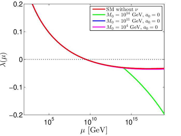
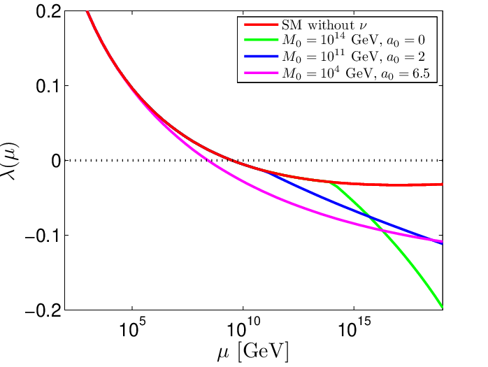
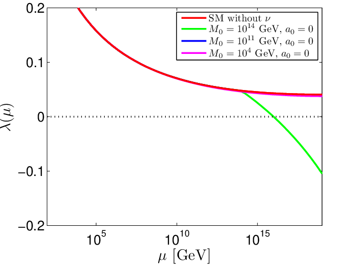
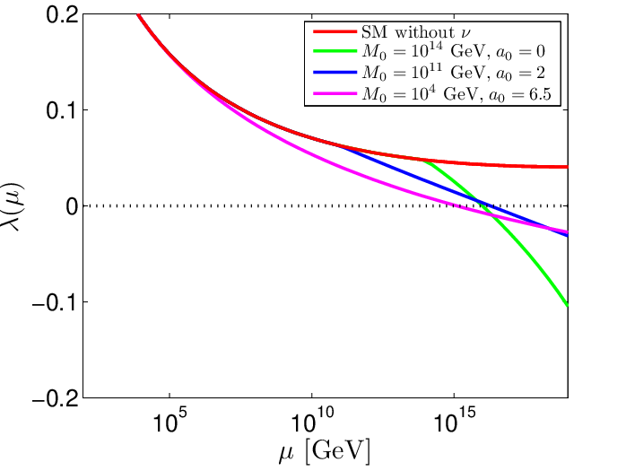
In Fig. 1 we show the impact of right-handed neutrinos on the evolution of $\lambda(\mu)$. For illustration purpose, we take $m_{H}=125~{\rm GeV}$ and $m_{H}=135~{\rm GeV}$ together with the light neutrino mass $m_{1}=0.1~{\rm eV}$. The value 125 GeV corresponds to a situation in which even in the SM there is a non-trivial cutoff scale, whereas 135 GeV is for our parameter choice a value which in the absence of SM extensions causes no conceptual issues up to the Planck scale. The red curves in Fig. 1 show the running behavior in the pure SM case, from which one can see that for $m_{H}=125~{\rm GeV}$ the self-coupling $\lambda$ crosses zero at energy scales around $10^{10}~{\rm GeV}$, indicating an upper bound on the potential new physics scale. In case of $m_{H}=135~{\rm GeV}$, the SM is valid in principle up to the Planck scale. The green and blue curves show the running of $\lambda$ with right-handed neutrino mass scale $M_{0}=10^{11}~{\rm GeV}$ and $M_{0}=10~{\rm TeV}$, respectively. For the left plots, we switch off the $A$ matrix by setting $a_{0}=0$. As can be seen from the plot, the evolution of $\lambda$ is barely affected by right-handed neutrinos (the curves almost overlap with each other), which is consistent with our analytical analysis since $Y_{\nu}$ is small in order to compensate a light right-handed neutrino scale. However, when we switch on the real parameters in the $A$ matrix, the evolution of $\lambda$ is modified significantly after crossing the seesaw threshold. Even for relatively light right-handed neutrinos, one can see clearly the shift of the cutoff scale down to low energy ranges. Noteworthy is for instance that the case $m_{H}=135~{\rm GeV}$ (which is safe in the SM) can have an unstable vacuum. This can happen even in the canonical case without any non-trivial $R$, as can be seen by the green line corresponding to $M_{0}=10^{14}$ GeV [27].

The effect of right-handed neutrinos on the stability bounds is shown in Fig. 2 for particular choices of parameters. The threshold effects take place at $\mu=M_{0}$ and can be identified easily on the plot. In the SM framework, there is essentially no stability constraint for Higgs masses larger than about $130~{\rm GeV}$, whereas in the presence of right-handed neutrinos the cutoff scale $\Lambda$ is decreased significantly, in particular for low scale seesaw models with large $A$ matrix elements. For completeness, we also show in Fig. 2 the triviality bounds on the Higgs mass improved by including right-handed neutrinos, i.e., $\lambda(\mu)<4\pi$. As expected, there is very little effect from seesaw. One can read from the plot that the Higgs mass window becomes narrower when the right-handed neutrinos are added, which is mainly due to the strengthening of the stability bounds.

As mentioned above, in determining the cutoff scale of possible new physics, the neutrino Yukawas can be crucial and may affect $\beta_{\lambda}$ in a similar way as the top quark mass. We illustrate in Fig. 3 the allowed parameter ranges in the $m_{H}$–$M_{0}$ plane by choosing the light neutrino mass $m_{1}=0.1~{\rm eV}$ and $a_{0}=2$. One can read from the plot that, for a chosen Higgs mass smaller than $125~{\rm GeV}$, the cutoff scale is essentially not affected by right-handed neutrinos (cf. the horizontal lines at the bottom of Fig. 3), since the corresponding Yukawa couplings are not significant enough when right-handed neutrino thresholds are lighter than $10^{10}~{\rm GeV}$. The situation becomes more complicated for a Higgs mass in the intermediate range, i.e., $130~{\rm GeV}\lesssim m_{H}<180\lesssim{\rm GeV}$, owing to the fact that there is essentially no stability constraint in the pure SM framework (i.e., $\Lambda$ can be as large as the Planck scale $10^{19}~{\rm GeV}$). For example, if the Higgs mass is located at $m_{H}=140~{\rm GeV}$, the cutoff scale $\Lambda$ decreases with increasing $M_{0}$, because $Y_{\nu}$ becomes larger in this case. When $\Lambda\gtrsim M_{0}$, $\Lambda$ stops decreasing and achieves a minimum, which can be seen from the plot for right-handed neutrino masses around a critical scale $M^{\rm cric}_{0}\sim 10^{12}~{\rm GeV}$. This can be easily understood because $\Lambda$ cannot be smaller than $M_{0}$, otherwise the right-handed neutrino threshold will not be crossed.²² 2 Note that a negative $\lambda$ arises for $\Lambda<M_{0}$, which, however, does not necessarily mean that the model is invalid, since the unlikely possibility of a metastable electroweak vacuum exists. For a general discussion on this topic, see, e.g. Ref. [13]. Then, for right-handed neutrino masses in the range $M_{0}>M^{\rm cric}_{0}$, the RG evolution between $M_{0}$ and $\Lambda$ is strongly enhanced by larger $Y_{\nu}$, which drives $\lambda$ to zero very efficiently, even for a small energy interval. Therefore, the cutoff $\Lambda$ will remain close to $M_{0}$, which is reflected in Fig. 3 by the vertical parts of the contour $\Lambda=10^{13}~{\rm GeV}$. Finally, when $m_{H}>180~{\rm GeV}$, $\Lambda$ is mainly constrained by the triviality bounds (cf. the horizontal lines at the top of Fig. 3). We should note that the features discussed here do not rely on the specific choice of model parameters. In general, the value of $M^{\rm cric}_{0}$ decreases with decreasing $a_{0}$.

We also show in Fig. 4 the parameter space of $M_{0}$ and $a_{0}$ constrained by the stability bound for $m_{H}=125~{\rm GeV}$ and $135$ GeV. From the plot one observes that the role of right-handed neutrinos becomes visible in case of a relatively large $a_{0}$ (e.g., $a_{0}>4$). In general, for a chosen $M_{0}$, the larger $a_{0}$ the smaller the cutoff scale one can expect. Interestingly, when both $M_{0}$ and $a_{0}$ are sizable, $\Lambda$ remains close to the right-handed neutrino masses ($\Lambda\simeq M_{0}$), due to the same reason mentioned in the above paragraph. This feature is shown by the vertical curves.

The RG evolution of $\lambda$ depends also on the light neutrino masses as can be seen in Eq. (10). Thus, we illustrate in Fig. 5 the dependence of $\Lambda$ on the lightest neutrino mass $m_{1}$. One can observe from the plot that, for a chosen right-handed neutrino scale, the larger the light neutrino mass, the lower the value at which $\Lambda$ could be located. This is in good agreement with our analytical results [cf. Eqs. (10) and (11)]. Moreover, $\Lambda$ is very sensitive to $a_{0}$, in particular when $a_{0}$ is large. Note however that $a_{0}$ cannot be arbitrarily large since $Y_{\nu}$ suffers from the perturbativity constraint. Furthermore, when right-handed neutrinos are relatively light (e.g. $\lesssim 10~{\rm TeV}$), the unitarity of the PMNS matrix $U$ sets constraints on the mixing between light and heavy neutrinos, suggesting roughly $(Y_{\nu}v/M_{0})^{2}\mathrel{\hbox to0.0pt{\raise 2.20013pt\hbox{$<$}\hss}{\lower 2.20013pt\hbox{$\sim$}}}10^{-3}$ [43, *Bekman:2002zk].

While the discussion made so far used a general parametrization of the unknown neutrino Yukawas, specific models or frameworks constructed in order to predict certain features of lepton mixing will be able to provide more definite information on the flavor structure. We will shortly discuss two examples. Both of them were constructed in order to have sizable cross sections for the production of heavy neutrinos at the LHC.

Model A: We first consider an $A_{4}$ type I seesaw model described in Ref. [31], in which right-handed neutrinos are assigned to the three-dimensional representation of $A_{4}$ while lepton doublets transform under ${\bf 1}^{\prime\prime}$. At leading order, $Y_{\nu}$ is given by

with $\omega=e^{{\rm i}\frac{2}{3}\pi}$, and the right-handed neutrino mass matrix is proportional to a unit matrix, i.e., $M_{R}=M_{0}\mathbbm{1}$. Using the seesaw formula (5), one can easily see that light neutrinos are massless in the leading order approximation. Small perturbations or explicit symmetry breaking terms are therefore needed to include neutrino masses. We can ignore them for the purpose of our study. The neutrino contribution to $\beta_{\lambda}$ is estimated by

As an example, we take $h_{1}=h_{2}=h_{3}=0.15$ together with $M_{0}=350~{\rm GeV}$, for which a discovery search can be performed at the LHC [42]. We illustrate in Fig. 6 the effect of right-handed neutrinos on the RG evolution of $\lambda$. Similar to Fig. 1, the right-handed neutrino corrections are noteworthy compared to the SM evolution.

Model B: Next we consider the minimal TeV seesaw model [32, *Zhang:2009ac], in which only two right-handed neutrinos are introduced, having opposite CP parity. In this model, right-handed neutrinos can be paired together to form a pseudo-Dirac fermion, and light neutrinos are massless at leading order due to the conservation of lepton number. Effectively, at leading order, the Yukawa coupling matrix is given by

while the right-handed mass matrix takes a $2\times 2$ form,

It is not difficult to calculate that³³ 3 Note that diagonalization of $M_{R}$ is not necessary, because the unitary matrix $V$ that diagonalizes it will appear together with $Y_{\nu}$ as $VY_{\nu}$ and thus drops out of $Y^{\dagger}_{\nu}Y_{\nu}$.

The running of $\lambda$ for the parameter choice $y_{1}=y_{2}=y_{3}=0.15$ is shown in Fig. 6. In comparison to model A, a factor $3$ is missing in ${\rm tr}\left(Y^{\dagger}_{\nu}Y_{\nu}\right)$, and therefore the modification to the running of $\lambda$ is milder.

Note that, in order to accommodate non-vanishing neutrino masses in those models, small lepton number violating perturbations have to be introduced [31, 32, *Zhang:2009ac, 34, *Ohlsson:2010ca, *Ibarra:2011xn, *Haba:2011pe], whose stability has to be guaranteed by symmetries. Explicitly, in order to generate sub-eV light neutrino masses, one needs perturbation terms $\epsilon$ in the Yukawa matrix of the order $\epsilon\sim\frac{m_{\nu}M_{R}}{y_{i}v^{2}}$. Taking Model B as an example, we can estimate that $\epsilon\sim 10^{-11}$. The mechanism behind this stability and the precise values of the parameters do not affect the main results of this work.

The Dirac Yukawas influence all $\beta$-functions of the SM, in particular the one of the top quark Yukawa coupling $y_{t}$. Its $\beta$-function approximately reads [47, *Machacek:1983fi, *Machacek:1984zw, *Arason:1991ic, *Ford:1992mv, *Luo:2002ey]

at energy scales above the right-handed neutrino threshold. Recall that, in the SM, the top quark Yukawa coupling tends to be smaller at higher energy scale due to the negative contribution of gauge couplings in $\beta_{y_{t}}$ (see e.g., [46]). Since the neutrino Yukawas contribute with a positive sign, the running behavior of $y_{t}$ may be significantly modified. The RG evolution of $y_{t}$ is depicted in Fig. 7 for some examples. An interesting observation is that the exact value $y_{t}=1$ (which is impossible in the SM) could be obtained at higher energy scales, indicating the restoration of certain kinds of Yukawa unifications or flavor symmetries. We see that this value can be reached for the case of low scale seesaw with non-trivial flavor structure as well as for the canonical case with $M_{0}$ being of order $10^{14}~{\rm GeV}$.