Learning Feature Hierarchies with Centered Deep Boltzmann MachinesThanks: Also at the Department of Brain and Cognitive Engineering, Korea University, Anam-dong, Seongbuk-gu, Seoul 136-713, Korea

Deep Boltzmann machines (Salakhutdinov and Hinton, 2009, DBM,) are in principle powerful models for extracting the hierarchical structure of data (Montavon et al., 2012). Unfortunately, attempts to train layers jointly (without greedy layer-wise pretraining) have been mostly unsuccessful. As we will argue later in greater detail, a possible reason for this could be that the mapping of net activities onto the sigmoid nonlinearities is not centered to zero by default.

In this paper, we propose to recenter the output of each unit to zero by rewriting the energy as a function of centered states $\xi=x-\beta$ where $\beta$ is an offset parameter. The reparameterization of the energy function leads to a better conditioned Hessian of the estimated model log-likelihood. The centered Boltzmann machine is easy to implement as the reparameterization leaves the associated Gibbs distribution invariant.

We train a centered deep Boltzmann machine on the MNIST data set. Empirical results show that the centered DBM is able to learn a top-layer representation that contains useful discriminative features and to produce a good generative model of data. In addition, the centered DBM learns faster and is more stable than its non-centered counterpart.

In this section, we introduce the centered Boltzmann machine. In the following, the sigmoid function is defined as $\text{sigm}(x)=\frac{e^{x}}{e^{x}+1}$, $x\sim\mathcal{B}(p)$ denotes that the variable $x$ is drawn randomly from a Bernouilli distribution of parameter $p$ and $\langle\cdot\rangle_{P}$ denotes the expectation operator with respect to a probability distribution $P$. All these operations apply element-wise to the input vector.

A Boltzmann machine is a network of $M_{x}$ interconnected binary units that associates to each state $x\in\{0,1\}^{M_{x}}$ the energy

$\displaystyle E(x;\theta)=-x^{\top}Wx-x^{\top}b$

where $\theta=\{W,b\}$ groups the model parameters. The matrix $W$ of size $M_{x}\times M_{x}$ is symmetric and contains the connection strength between units. The vector $b$ of size $M_{x}$ contains the biases associated to each unit. A probability is associated to each state according to the Gibbs distribution

$\displaystyle p(x;\theta)=\frac{e^{-E(x;\theta)}}{\sum_{x}e^{-E(x;\theta)}}$

where the term in the denominator is the partition function that makes probabilities sum to one. For the centered Boltzmann machine, we rewrite the energy as a function of centered states

$\displaystyle E(x;\theta)=-(x-\beta)^{\top}W(x-\beta)-(x-\beta)^{\top}b$

where $\theta=\{W,b,\beta\}$ and where the vector $\beta$ contains the offsets associated to each unit of the network. Setting $\beta=\text{sigm}(b_{0})$ where $b_{0}$ is the initial bias enforces the initial centering of the Boltzmann machine. From these equations, we can derive the conditional probability

$\displaystyle p(x_{i}=1|x_{-i};\theta)=\text{sigm}(b_{i}+\sum_{j\neq i}W_{ij}(x-\beta)_{j})$

of each unit and the gradient of the model log-likelihood with respect to $W$ and $b$:

	$\displaystyle\frac{\partial}{\partial W}\langle\log p(x;\theta)\rangle_{\text{data}}$	$\displaystyle=\langle(x-\beta)(x-\beta)^{\top}\rangle_{\text{data}}-\langle(x-\beta)(x-\beta)^{\top}\rangle_{\text{model}}$
	$\displaystyle\frac{\partial}{\partial b}\langle\log p(x;\theta)\rangle_{\text{data}}$	$\displaystyle=\langle x-\beta\rangle_{\text{data}}-\langle x-\beta\rangle_{\text{model}}$

We present the method introduced by Montavon et al. (2011) that measures how the representation evolves layer after layer in a deep network. It is based on the theoretical insight that the projection of the input distribution onto the hidden units of each layer provides a function space that can be thought of as a representation or a feature extractor.

The method aims to characterize this function space by constructing a kernel for each layer that approximates the implicit transfer function between the input and the layer and measuring how much these kernels “match” the task of interest. The approach is theoretically motivated by the work of Braun et al. (2008) showing that projections on the leading components of the implicit kernel feature map (Schölkopf et al., 1998) obtained with a finite and typically small number of samples $n$ are close with essentially multiplicative errors to their asymptotic counterparts. In the following lines, we describe the principal steps of the analysis:

Let $X$ and $T$ be two matrices of $n$ rows representing respectively the inputs and labels of a data set of $n$ samples. Let

$\displaystyle f:x\mapsto f_{L}\circ\dots\circ f_{1}(x)$

be a deep network of $L$ layers. We build a hierarchy of increasingly “deep” kernels

	$\displaystyle k_{0,\sigma}(x,x^{\prime})$	$\displaystyle=\kappa_{\sigma}(x,x^{\prime})$
	$\displaystyle k_{1,\sigma}(x,x^{\prime})$	$\displaystyle=\kappa_{\sigma}(f_{1}(x),f_{1}(x^{\prime}))$
		$\displaystyle~\>\vdots$
	$\displaystyle k_{L,\sigma}(x,x^{\prime})$	$\displaystyle=\kappa_{\sigma}(f_{L}\circ\dots\circ f_{1}(x),f_{L}\circ\dots\circ f_{1}(x^{\prime}))$

that subsume the mapping performed by more and more layers of the deep network and where $\kappa_{\sigma}$ is an RBF kernel of scale $\sigma$. For each kernel $k_{l,\sigma}$, we can compute the empirical kernel $K_{l,\sigma}$ of size $n\times n$ and its eigenvectors $u_{l,\sigma}^{1},\dots,u_{l,\sigma}^{n}$ sorted by decreasing magnitude of their respective eigenvalues $\lambda_{l,\sigma}^{1},\dots,\lambda_{l,\sigma}^{n}$.

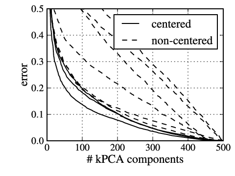
We measure how good a representation is with respect to a certain task by measuring whether the task is contained within the leading principal components of the representation. The matrix

$\displaystyle U_{l,\sigma}^{d}=(u_{l,\sigma}^{1}\mid\dots\mid u_{l,\sigma}^{d})$

spans the $d$ leading kernel principal components of empirical kernel. The error is obtained as the residuals of the projection of the labels $T$ on the $d$ leading components of the mapped distribution:

$\displaystyle e_{T}(l,d,\sigma)=||T-U_{l,\sigma}^{d}{U_{l,\sigma}^{d}}^{\!\!\!\top}T||_{F}^{2}$

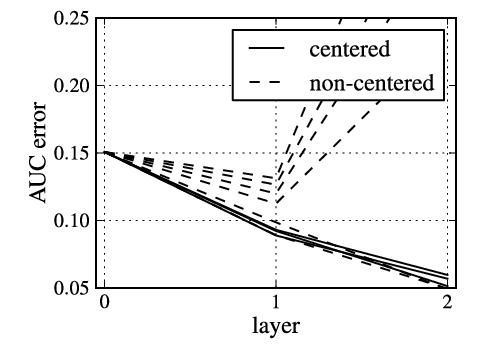
Curves $(e(l,0,\sigma),\dots,e(l,d,\sigma))$ represent how well the task can be solved as we add more and more principal components of the data distribution. These curves can be interpreted as learning curves as the regularization imposed by the rank of the kernel feature space determines the number of samples that are necessary in order to train the model effectively. Therefore, the number of observed kernel principal components $d$ closely relates to the amount of label information given to the learning machine. Small values for $d$ cover the “one-shot” learning regime where the model is asked to generalize from very few observations. On the other hand, large values for $d$ cover the other extreme case where label information is abundant, and where the representation has to be rich enough in order to encode any subtle variation of the learning problem. For practical purposes, these curves can be reduced as follows:

	$\displaystyle e_{T}(l,d)$	$\displaystyle=\min_{\sigma}e_{T}(l,d,\sigma)$		(5)
	$\displaystyle e_{T}(l)$	$\displaystyle=\frac{1}{n}\sum_{d=1}^{n}e_{T}(l,d)$		(6)

These compact measures of how well layer $l$ represent $T$ make it easier to compare the layer-wise evolution of the representation for different architectures.

Here, we present an analysis that estimates the likelihood of the learned Boltzmann machine (Salakhutdinov and Hinton, 2010) based on annealed importance sampling (Neal, 2001, AIS,). We describe here the basic analysis. Salakhutdinov and Hinton (2010) introduced more elaborate procedures for particular types of Boltzmann machines such as restricted, semi-restricted and deep Boltzmann machines.

A deep Boltzmann machine associates to each input $x$ a probability

$\displaystyle p(x;\theta)=\frac{\Psi(\theta,x)}{Z(\theta)}$

	$\displaystyle\text{where}\quad\Psi(\theta,x)$	$\displaystyle=\sum_{y,z}p^{\star}(x,y,z;\theta)$
	$\displaystyle Z(\theta)$	$\displaystyle=\sum_{x,y,z}p^{\star}(x,y,z;\theta)$

and where $p^{\star}(x,y,z;\theta)=e^{-E(x,y,z;\theta)}$ is the unnormalized probability of state ($x,y,z$). Computing $\Psi(\theta,x)$ and $Z(\theta)$ analytically is intractable because of the exponential number of elements involved in the sum. Let us rewrite the ratio of partition functions as follows:

$\displaystyle p(x;\theta)$

$\displaystyle=\frac{\Psi(\theta,x)}{Z(\theta)}=\frac{\frac{\Psi(\theta,x)}{\Psi(0,x)}}{\frac{Z(\theta)}{Z(0)}}\cdot\frac{\Psi(0,x)}{Z(0)}$

(7)

It can be first noticed that the ratio of base-rate partition functions ($\theta=0$) is easy to compute as $\theta=0$ makes units independent. It has the analytical form

$\displaystyle\frac{\Psi(0,x)}{Z(0)}=\frac{1}{2^{M_{x}}}.$

(8)

The two other ratios in Equation 7 can be estimated using annealed importance sampling. The annealed importance sampling method proceeds as follows:

Annealed importance sampling: 1. Generate a sequence of states $\xi_{1},\dots,\xi_{T}$ using a sequence of transition operators $\mathcal{T}(\xi,\xi^{\prime};\theta_{0}),\dots,\mathcal{T}(\xi,\xi^{\prime};\theta_{K})$ that leave $p(\xi)$ invariant, that is, • Draw $\xi_{0}$ from the base model (e.g. a random vector of zero and ones) • Draw $\xi_{1}$ given $\xi_{0}$ using $\mathcal{T}(\xi,\xi^{\prime};\theta_{1})$ • $\dots$ • Draw $\xi_{K}$ given $\xi_{K-1}$ using $\mathcal{T}(\xi,\xi^{\prime};\theta_{K})$ 2. Compute the importance weight $\displaystyle\omega_{\text{AIS}}=\frac{p^{\star}(\xi_{1};\theta_{1})}{p^{\star}(\xi_{1};\theta_{0})}\cdot\frac{p^{\star}(\xi_{2};\theta_{2})}{p^{\star}(\xi_{2};\theta_{1})}\cdot\dots\cdot\frac{p^{\star}(\xi_{K};\theta_{K})}{p^{\star}(\xi_{K};\theta_{K-1})}$

It can be shown that if the sequence of models $\theta_{0},\theta_{1},\dots,\theta_{K}$ where $\theta_{0}=0$ and $\theta_{K}=\theta$ evolves slowly enough, the importance weight obtained with the annealed importance sampling procedure is an estimate for the ratio between the partition function of the model $\theta$ and the partition function of the base rate model.

In our case, $\xi$ denotes the state $(x,y,z)$ of the DBM and the transition operator $\mathcal{T}(\xi,\xi^{\prime};\theta)$ is the alternate Gibbs sampler defined in Equation 3. We can now compute the two ratios of partition functions of Equation 7 as

$\displaystyle\frac{Z(\theta)}{Z(0)}\approx\text{E}[\omega_{\text{AIS}}]\quad\text{and}\quad\frac{\Psi(\theta,x)}{\Psi(0,x)}\approx\text{E}[\nu_{\text{AIS}}(x)]$

(9)

where $\omega_{\text{AIS}}$ is the importance weight resulting from the annealing process with the freely running Gibbs sampler and $\nu_{\text{AIS}}$ is the importance weight resulting from the annealing with input units clamped to the data point. Substituting Equation 8 and 9 into Equation 7, we obtain

$\displaystyle p(x;\theta)\approx\frac{\text{E}[\nu_{\text{AIS}}(x)]}{\text{E}[\omega_{\text{AIS}}]}\cdot\frac{1}{2^{M_{x}}}$

and therefore, the log-likelihood of the model is

$\displaystyle\text{E}_{X}[\log(p(x;\theta))]\approx\text{E}_{X}[\log\text{E}[\nu_{\text{AIS}}(x)]]-\log\text{E}[\omega_{\text{AIS}}]-M_{x}\log(2).$

(10)

Generally, computing an average of the importance weight $\nu_{\text{AIS}}$ for each data point $x$ can take a long time. In practice, we can use an approximation to this computation where the estimate is computed with a single AIS run for each point. In that case, it follows from Jensen’s inequality that

$\displaystyle\text{E}_{X}[\log\nu_{\text{AIS}}(x)]-\log\text{E}[\omega_{\text{AIS}}]\leq\text{E}_{X}[\log\text{E}[\nu_{\text{AIS}}(x)]]-\log\text{E}[\omega_{\text{AIS}}].$

(11)

Consequently, this approximation tends to produce slightly pessimistic estimates of the model log-likelihood, however the variance of $\nu_{\text{AIS}}$ is low compared to the variance of $\omega_{\text{AIS}}$ because the clamping of visible units to data points sharply reduces the diversity of AIS runs. We find that this approximation is sufficiently accurate for the purpose of this paper, that is, demonstrating the importance of centering deep Boltzmann machines.

In this section, we describe the different parameters used to train the deep Boltzmann machines and to perform the discriminative and generative analysis. These parameters correspond to reasonable choices, most of which have been validated by previous research work.

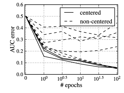
Table 1 corroborates the importance of centering for better discriminating in the top layer of a deep Boltzmann machine. As it can be seen in Figure 5 (left), discriminative performance of the top layer can be further improved by training the network for a longer time.

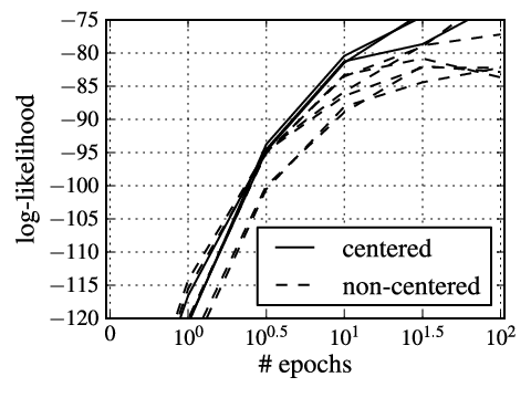
Table 2 further supports the importance of centering, showing that centered DBMs learn a better generative model of data. However, the advantage is not as strong as for the discriminative case. Indeed, units in the top layer are not critical for generative performance as the learning algorithm can simply discard them and learn a one-layer shallow generative model instead.

Figure 5 and 5 highlight the importance of centering for faster and more stable learning. The models emerging from the centered deep Boltzmann machine have systematically better discriminative properties in the top layer and good generative properties. While a non-centered DBM may ultimately learn a model which is as good as the one produced by a centered DBM, it may also diverge.

Figure 8 and 8 show that each model is able to learn reasonable first-layer filters but that second-layer filters learned by a centered DBM tend to be more varied than those learned by a non-centered DBM. This higher variety of second layer filters suggests that the centered DBM produces a richer top-level representation. The argument is corroborated by Figure 9 showing that, in absence of centering mechanism, the projection of the data on the top layer representation tends to form a simplistic low-dimensional manifold that may still contain useful features (for example, discriminating the digit “1” from other digits) but, on the other hand, that also discards a lot of potentially useful discriminative features. As suggested by Figure 8, the top-layer simplistic representation may even negatively affect the generative properties of the model by perturbing the balance between different classes.

We presented a simple modification of the deep Boltzmann machine that centers the output of the sigmoids by rewriting the energy function as a function of centered states. This centered version of the deep Boltzmann machine is easy to implement as it simply involves a reparameterization of the energy function. A theoretical motivation for centering is that it leads to a better conditioning of the Hessian of the optimization criterion.

This simple modification allows to learn efficiently a deep Boltzmann machine without greedy layer-wise pretraining. Experiments on real data corroborate the benefits of centering, showing that the centered deep Boltzmann machine learns faster and is more stable than its non-centered counterpart. In addition, the centered deep Boltzmann machine produces useful discriminative features in the top layer and a good generative model of data.

Training hierarchies of many layers is still tedious and requires many iterations. Understanding whether the difficulty comes from a difficult optimization problem or from the exhaustion of statistical information in the data set remains to be done. Also, despite an initial good conditioning of the Hessian, it can not be excluded that the solution progressively drifts towards degenerate regions of the parameter space throughout the learning procedure. Strategies to dynamically maintain the solution within well-behaved regions of the parameter space or to better descend the objective function also need to be further investigated.

References

- Braun et al. (2008) Mikio L. Braun, Joachim Buhmann, and Klaus-Robert Müller. On relevant dimensions in kernel feature spaces. Journal of Machine Learning Research, 9:1875–1908, Aug 2008.
- Glorot and Bengio (2010) Xavier Glorot and Yoshua Bengio. Understanding the difficulty of training deep feedforward neural networks. Journal of Machine Learning Research - Proceedings Track, 9:249–256, 2010.
- Hinton (2010) Geoffrey E. Hinton. A practical guide to training restricted Boltzmann machines. Technical report, University of Toronto, 2010.
- LeCun et al. (1998) Yann LeCun, Léon Bottou, Genevieve B. Orr, and Klaus-Robert Müller. Efficient backprop. In Genevieve B. Orr and Klaus-Robert Müller, editors, Neural Networks—Tricks of the trade LNCS 1524, pages 5–50. Springer, 1998.
- Montavon et al. (2011) Grégoire Montavon, Mikio L. Braun, and Klaus-Robert Müller. Kernel analysis of deep networks. Journal of Machine Learning Research, 12:2563–2581, 2011.
- Montavon et al. (2012) Grégoire Montavon, Mikio L. Braun, and Klaus-Robert Müller. Deep Boltzmann machines as feed-forward hierarchies. In International Conference on Artificial Intelligence and Statistics (AISTATS), 2012.
- Neal (2001) Radford M. Neal. Annealed importance sampling. Statistics and Computing, 11(2):125–139, 2001.
- Pearlmutter (1994) Barak A. Pearlmutter. Fast exact multiplication by the Hessian. Neural Computation, 6(1):147–160, 1994.
- Polyak and Juditsky (1992) Boris T. Polyak and Anatoly B. Juditsky. Acceleration of stochastic approximation by averaging. Siam J. Control Optim, 30(4):838–855, 1992.
- Salakhutdinov and Hinton (2009) Ruslan Salakhutdinov and Geoffrey E. Hinton. Deep Boltzmann machines. In Proceedings of the International Conference on Artificial Intelligence and Statistics, volume 5, pages 448–455, 2009.
- Salakhutdinov and Hinton (2010) Ruslan Salakhutdinov and Geoffrey E. Hinton. An efficient learning procedure for deep Boltzmann machines. Technical Report MIT-CSAIL-TR-2010-037, MIT, 2010.
- Schölkopf et al. (1998) Bernhard Schölkopf, Alexander Smola, and Klaus-Robert Müller. Nonlinear component analysis as a kernel eigenvalue problem. Neural Computation, 10(5):1299–1319, 1998.
- Tang and Sutskever (2011) Yichuan Tang and Ilya Sutskever. Data normalization in the learning of restricted Boltzmann machines. Technical Report UTML-TR-11-2, Department of Computer Science, University of Toronto, 2011.
- Tieleman (2008) Tijmen Tieleman. Training restricted Boltzmann machines using approximations to the likelihood gradient. In Proceedings of the 25th International Conference on Machine Learning, pages 1064–1071, 2008.
- Tieleman and Hinton (2009) Tijmen Tieleman and Geoffrey E. Hinton. Using fast weights to improve persistent contrastive divergence. In Proceedings of the 26th international conference on Machine learning, pages 1033–1040, 2009.
- Xu (2011) Wei Xu. Towards optimal one pass large scale learning with averaged stochastic gradient descent. CoRR, abs/1107.2490, 2011.