Randomized Benchmarking of Multi-Qubit Gates
Abstract
As experimental platforms for quantum information processing continue to mature, characterization of the quality of unitary gates that can be applied to their quantum bits (qubits) becomes essential. Eventually, the quality must be sufficiently high to support arbitrarily long quantum computations. Randomized benchmarking already provides a platform-independent method for assessing the quality of one-qubit rotations. Here we describe an extension of this method to multi-qubit gates. We provide a platform-independent protocol for evaluating the performance of experimental Clifford unitaries, which form the basis of fault-tolerant quantum computing. We implemented the benchmarking protocol with trapped-ion two-qubit phase gates and one-qubit gates and found an error per random two-qubit Clifford unitary of , thus setting the first benchmark for such unitaries. By implementing a second set of sequences with an extra two-qubit phase gate at each step, we extracted an error per phase gate of . We conducted these experiments with movable, sympathetically cooled ions in a multi-zone Paul trap—a system that can in principle be scaled to larger numbers of ions.
I Introduction
Quantum information processing (QIP) has the potential to solve difficult problems in many-body quantum mechanics and mathematics that lack efficient algorithms on classical computers. However, achieving useful QIP will require precise control of many qubits (two-level quantum systems) and the ability to execute quantum gates (operations that manipulate the quantum states of the qubits) with low error per gate. Here, the error per gate (EPG) is , where is the (average) gate fidelity defined as the uniform average over pure input states of , where is the (typically mixed) output state and is the intended output state (see Ref. [1]). A convincing demonstration of the potential for practical fault-tolerant QIP should include verification of consistent EPGs below a threshold of [2, 3].
So far, there has been substantial experimental progress on the basic techniques needed for QIP, including the manipulation of small numbers of qubits and the implementation of the basic quantum gates that are needed to perform useful algorithms [4]. The main challenges for QIP experiments that remain are to scale up to larger numbers of qubits and to decrease the EPG below the fault-tolerant threshold. Therefore, it is desirable to efficiently characterize or benchmark the performance of multi-qubit QIP experiments so as to extract the EPG of specific gates and enable comparison between different quantum computing platforms. With these goals in mind, we give a benchmarking protocol for arbitrary numbers of qubits and show the results from an experimental implementation for two qubits. The protocol builds on previous work that used randomized sequences of Clifford gates to measure the EPG of one-qubit gates, first implemented in Refs. [5, 6].
Compared to techniques such as process tomography [7, 8], randomized benchmarking offers several key advantages for characterizing EPGs of quantum gates. For example, while process tomography offers more complete information about the performance of a gate, it does not scale efficiently with the number of qubits in the system, it cannot readily measure EPGs below the error probabilities of state preparation and readout, and it does not verify performance of a gate in arbitrary computational contexts. In contrast, randomized benchmarking can determine EPGs with a number of measurements that scales polynomially with the number of qubits [5, 9]. Because randomized benchmarking measures an exponential decay of fidelity as a function of the number of gates in the sequences, errors in state preparation and readout do not limit the minimum EPG that one can measure. Also, randomized benchmarking involves gates in the context of long sequences of operations and therefore establishes an EPG that takes into consideration a computational context similar to that expected in the implementation of lengthy QIP algorithms. Because of these advantages, randomized benchmarking following the protocols of Refs. [5, 6] has been used to measure one-qubit gate errors in a range of systems including trapped ions [5, 10], superconducting qubits [11, 12], liquid-state NMR [6], and neutral atoms in an optical lattice [13]. Recently, randomized benchmarking was used to measure an EPG of for one-qubit operations with a trapped ion [10].
A number of previous works have described properties of two-qubit gates with various measurement techniques. With trapped ions, the fidelity for creating a Bell state has been measured at [14], [15], [16], [17] and [18]. Process tomography was used to look at single and repeated applications of a two-qubit entangling gate [19, 20]. The average fidelities were found to be for one and for two gates in Ref. [20]. Two-qubit gates have also been studied in other quantum computing platforms including superconducting and photonic qubits (see Ref. [4] and citations therein), with measured fidelities ranging from to , disregarding photon loss for photonic qubits. In a liquid-state NMR system, a randomized benchmarking technique was used to study the errors of sequences of randomized gates on three nuclear spins [6] and found EPGs of . The gates in this experiment were randomly chosen in a platform-dependent way from a special-purpose probability distribution where the probability of a two-qubit gate (the CNOT) was . However, gate sets vary by platform, and other experiments may choose different probability distributions, for example to improve randomization. As a result the error probabilities from Ref. [6] may be difficult to compare to those obtained in future experiments.
The multi-qubit protocol we describe first establishes a platform-independent error per operation (EPO) 11 1 We use the convention that EPGs refer to processes that are intended to implement elementary quantum gates, whereas EPOs refer to processes that implement quantum circuits that may scale with the number of qubits. In both cases, the gates or circuits need to be specified to interpret reported values. for Clifford unitaries by applying random sequences of Clifford unitaries of varying lengths. Here, a Clifford unitary is any operator in the Clifford group defined below. It then determines the EPG of individual gates of our choice by inserting them into these sequences. The individual gates to be characterized may depend on the platform. Of particular interest are implementations of one of the standard universal two-qubit gates such as the controlled-not (CNOT), phase gate or square-root of swap. The basic principles of the protocol are similar to the theoretical randomized Clifford-based benchmarking sequences described and analyzed in Ref. [9]. However, like the standard protocol used in one-qubit benchmarking experiments so far, the last gate of the sequence does not strictly reverse the effects of the previous ones, thus enabling the protocol to detect certain large errors that can otherwise masquerade as no errors. In addition, we discuss the practical aspects of choosing the random Clifford unitaries in the sequence and extend the protocol to enable characterization of specific gates, thus enabling diagnostics that were previously unavailable in randomized benchmarking. The proposed protocol is flexible without affecting the ability to compare results from unrelated implementations. We note that the theoretical relationship between the protocol’s EPGs and EPOs and the detailed physical noise parameters is not known in general [9]. However, we suggest that subject to simple consistency checks, the protocol’s reported EPGs and EPOs are nevertheless useful quantities for comparison and reflect computationally relevant error behavior.
For our demonstration with trapped ions, we take advantage of a multi-zone ion trap [21]. The universal two-qubit gate chosen here is a phase gate, , implemented via a Mølmer-Sørensen gate [22] and acting as the diagonal matrix with diagonal in the basis labeled by ,,,, where and represent the two eigenstates of each qubit, with , etc. Qubit addressing is implemented by separation of the ions into different wells, and long sequences of gates are supported by sympathetic cooling techniques as required for the approach to scalable ion-trap quantum computing described in Refs. [23, 24]. The experiment extends the technology demonstrated in [20] by using longer sequences of gates and a different implementation of the phase gate [25] to act directly on a magnetic-field-insensitive transition in 9Be+.
From sequences of up to seven Clifford unitaries, each requiring an average of phase gates, we deduced an EPO of for the Clifford unitaries and an EPG of for the phase gates. Although we implemented relatively long sequences, the experiment does not yet demonstrate stationary behavior because ion loss prevented routine implementation of longer sequences. There are also indications that the errors increased with sequence length by two to three standard deviations, with the EPOs ranging from to and the EPGs from to as the sequences lengthened. Our EPO sets the first benchmark for random two-qubit Clifford unitaries. The EPG shows no improvement over the gates used in [20], but applies to gates used in computationally relevant contexts in longer sequences.
The paper is structured as follows: We first describe the protocol and its main features for two qubits. We then discuss the experimental implementation of the protocol and show the experimental results. The data-analysis methods are detailed next, followed by a discussion of necessary consistency checks and estimates of physical sources of error. We finally define the protocol for arbitrary numbers of qubits, and make recommendations for how to apply and compare it when qubit numbers vary.
II Benchmarking Protocol
Clifford unitaries are fundamental to most error-correcting procedures envisioned for quantum computing (see, for example, Ref. [26]) and thus serve as a foundation on which universal fault-tolerant quantum computing is built. As a result, a large fraction of the fundamental processes in proposed quantum computing architectures involve Clifford unitaries. The three main features of the group of Clifford unitaries that make it useful for our purposes are that its members have compact representations that can be efficiently converted to circuits of elementary quantum gates, outcomes of standard measurements of sequences of Clifford unitaries can be efficiently predicted by classical computation, and the group is sufficiently rich that error operators can be perfectly depolarized. These features are explained in context below.
For a system of qubits, Clifford unitaries can be constructed by combining one-qubit rotations, defined as with , about the and axes, and two-qubit CNOT gates. Alternatively, the Clifford unitaries are the members of the Clifford group, which is defined as the set of unitaries with the property that for every Pauli operator , is a signed product of Pauli operators. We consider two gates or unitaries that differ only by a global phase to be identical.
The randomized benchmarking protocol is an extension of “Clifford twirling” [1]. In the simplest instance of Clifford twirling, an arbitrary quantum process is sandwiched between a random Clifford unitary picked from a uniform distribution and its inverse . Alternatively, we can think of Clifford twirling as averaging the process over all elements in the set , of Clifford unitaries. The key property of Clifford twirling is that this new process behaves like one that uniformly depolarizes with some probability. In other words, a single parameter, the probability that a pure input state is mapped to an orthogonal state, characterizes the new, average process [1]. When is a noisy implementation of the identity gate, such as a long self-reversing sequence of gates, we use this parameter as the definition of the average error of . Clifford twirling can be generalized to learn the average error of an arbitrary process intended to implement a specific Clifford unitary : The inverting Clifford unitary that is applied after the process is modified to an implementation of the unitary . With this modification, the net effect is if there are no errors in . Because Clifford unitaries form a group, is also Clifford. The implementation of should not rely on to provide , and it is better not to decompose it into a composition of three processes according to the given expression. This can be satisfied by first evaluating the unitary operator as an element of the Clifford group and then implementing it by an efficient procedures for translating Clifford unitaries into quantum circuits [27, 28]. If contains errors, then the net process applies the unitary followed by a uniformly depolarizing error whose parameter defines the average error of .
Randomized benchmarking extends the idea of Clifford twirling from the simple three-step sequence described above to randomized sequences of Clifford unitaries with errors. These sequences consist of steps where each step implements a randomly-chosen Clifford unitary and may have errors. Each step in the sequence simultaneously acts as a process that undergoes twirling and contributes to the twirling of errors in the other steps. Under optimistic assumptions described later, each step effectively behaves as an ideal unitary followed by a depolarizing process. The first goal is to establish the average error per step, which can then be reported as the EPO for Clifford unitaries.
The method for implementing the Clifford unitaries making up the steps in the randomized sequences is up to the experimenter. Here we describe our approach. To improve stability of the twirling process and take advantage of the typically lower errors of one-qubit gates, each step is composed of a Clifford unitary preceded by a Pauli unitary, where the two parts are chosen so that together they implement a uniformly random Clifford unitary. The choice of Pauli unitary on each qubit is random and independent from the choice of Clifford unitary; each Pauli unitary involves applying either no pulse or a major-axis -pulse. There are eight possible such pulses acting as , where is a Pauli matrix or the identity: , . The sign in the exponent affects only the global phase and results in two choices for each possible matrix in the exponent. We keep the sign because in many cases including ours, the change in sign can involve a physically different device setting, such as the phase in a pulse generator that determines the orientation of the fields that mediate the pulse. Each qubit’s pulse is chosen uniformly at random from the above eight pulses.
Because of this Pauli randomization procedure, it suffices to choose the unitary in the second part of the step uniformly at random from the Clifford group modulo the group of Pauli products. For this we can take advantage of the fact that the group of Pauli products is a normal subgroup of the Clifford group, and the quotient group (of Clifford unitaries modulo Pauli products) has a representation in terms of binary symplectic matrices of dimension such that modulo , where is a block matrix with blocks whose diagonal blocks are zero and whose off-diagonal blocks are the identity, see, for example Ref. [29, 30]. The terminology is based on Ref. [31]. For two qubits, there are such matrices . Uniformly and randomly choosing from among these matrices is computationally straightforward and efficient.
Determining an implementation of the Clifford unitary described by such a matrix in terms of the elementary gates available in a particular experiment is more challenging. There are efficient algorithms that translate an arbitrary symplectic binary matrix into order of elementary one- and two-qubit gates [27, 28], each of which can then be mapped into experimentally available operations. However, there is strong motivation to obtain shorter implementations, as this is a sure way to improve the measured EPO. While it is unlikely that optimal implementations can be readily obtained for arbitrary numbers of qubits, we used the following strategy for two qubits optimized for our demonstration: By exhaustively listing compact circuits of one-qubit Clifford gates and phase gates , we determined for each of the symplectic binary matrices a circuit with the minimum number of phase gates implementing the corresponding Clifford unitary (modulo a Pauli product). On average, phase gates were required. These circuits were then translated into appropriate actions in our ion-trap platform.
Given the method for generating the random unitaries for one step, a benchmarking experiment is configured by first deciding on a set of lengths that determine the numbers of steps in sequences to be generated. The EPO is determined by fitting an exponential decay to fidelities ( , where is the error probability) measured for each sequence length. The choice of lengths therefore contributes to how well the EPO can be extracted. In particular, there should be enough lengths for stable curve fitting, and lengths much greater than the inverse EPO contribute little additional information. For each length , many sequences of random steps are produced. At the end of each such sequence, a randomized measurement step is added. This step consists of a Pauli randomization followed by a Clifford unitary that inverts the preceding Clifford steps. The final Clifford unitary is chosen independently of the Pauli randomization. This ensures that in the absence of errors, the final state is again in the computational basis but randomized. Which basis element it should be in can be computed by use of standard efficient methods for simulating sequences of Clifford unitaries [29]. The sequence can then be experimentally implemented after preparation of each qubit in the eigenstate of and followed by a measurement in the basis of each qubit.
One should implement sufficiently many runs of each sequence to have good signal-to-noise on the inferred probabilities of getting a correct or incorrect answer in the measurement for this particular sequence. The process of generating and implementing random sequences at each length is repeated in order to ensure randomization of the unitaries and their associated implementation errors. For our two-qubit benchmarking demonstration, we used the set of lengths and generated between and random sequences of each length. The variation in numbers of sequences is explained below. We implemented runs for each sequence to determine its probability of error 22 2 Due to an undetermined problem in the control code, for approximately of experiments, the record for one run is missing. Thus, for experiments with nominally runs, occasionally only runs were recorded..
The experimental runs yield an average probability of error for each length , where the average is over the sequences of this length and their runs. To analyze we start by making the simple assumption that each step’s error behaves as a completely depolarizing channel (see, for example, Ref. [30], pg. 378) characterized by error probability independent of its gates or position in the sequence. Similarly, we assume an overall error probability for state preparation, the last inverting gate and its Pauli randomization, and measurement. Then the mean of with respect to repetitions of the experiment satisfies
| (1) |
for two qubits. The case of more than two qubits is discussed in Sec. VIII. Note that is the depolarization probability if the error probability is . The probability of not depolarizing the state in a sequence is the product of the probabilities of not depolarizing in each step. To derive the equation, note that in terms of , the probability of not depolarizing is .
Assuming that the experimental observations are consistent with the simple exponential behavior suggested by this formula, we use it as the defining formula for the EPO of a random Clifford unitary, regardless of the actual behavior of errors. In particular, in the context of these benchmarks, we associate the EPO with the decay parameter of the error probabilities rather than a particular exact parameter of the underlying physical errors. This supports the platform-independent use of randomized benchmarking. If the simple depolarizing assumption does not hold, then may exhibit non-exponential and transient behaviors; see the discussion below. However, the twirling effected by the randomization is intended to induce behavior that matches the one implied by this assumption.
To isolate the EPG of the phase gate (or any other gate) we generate a second set of sequences by inserting after each random Clifford unitary. The final inverting Clifford unitary is chosen in the same way as before, taking into account the effect of the additional gates to ensure that the final state is a predictable computational basis state in the absence of errors. Under the same idealizing assumptions that yield Eq. (1), the average probability of error measured for the implementation of this experiment satisfies Eq. 1, but with a different value of due to the additional operation in each step. In an ideal experiment should be the same, but the model must take into consideration that it might have changed, for example due to experimental drifts. Explicitly,
| (2) |
where is the probability of error of a step consisting of a random Clifford gate and . In this context, the assumptions on the error behavior of could be relaxed from simple depolarization. We can isolate the EPG of by solving the identity
| (3) |
which gives
| (4) |
It is helpful to run randomized benchmarks on subsets of the available qubits so that results can be compared to other experimental platforms that have different numbers of available computational qubits and for investigating differences in behavior that depend on (for example) geometrical relationships between qubits. If possible, these benchmarks should be run in parallel on disjoint subsets. For these reasons, we checked the performance of the one-qubit gates in parallel on the two ion qubits. Because of the pre-existing benchmarks, we did not implement the above protocol for each qubit, but used a one-qubit benchmarking protocol similar to that of Ref. [5]. Briefly, the length of a sequence is the number of steps that consist of a Pauli gate (-pulse) followed by a Clifford gate (-pulse) on each qubit. Each step can be thought of as implementing a random computational gate. The gate sequence is followed by a Pauli gate and Clifford gate chosen to yield a predictable measurement outcome in the basis for each qubit. The Pauli gates are chosen with equal probability to be rotations about the or axis or the identity. The Clifford gates are chosen with equal probability from the following five options: or the identity. When many subsequent gates are composed together, this distribution of Clifford gates demonstrates favorable convergence to a uniformly random Clifford unitary in comparison with the distribution in Ref. [5]. The introduction of identity gates into the Clifford gate step reduces the average expected number of -pulses in that step from to .
III Experimental Implementation
We perform the benchmarking demonstration with the ion-trap system described in [32, 20, 33] using updated techniques. This system includes most of the features of the scalable quantum computing architecture of [23, 24]. We trap four ions in a six-zone linear Paul trap: two 9Be+ ions that serve as the qubits, and two 24Mg+ ions that are used for sympathetically recooling the qubit ions during the sequences. The ions form a linear chain along the axis of the trap, which is the axis of weakest confinement. The two-qubit phase gates are performed with all four ions in the same trap zone, in the order 9BeMgMgBe+ (Fig. 2a bottom left). Individual addressing of the ions for one-qubit rotations is achieved by separating the ions into two trap zones apart with a single 9Be+-24Mg+ pair in each zone (Fig. 2a below electrodes).

The qubit states are the and hyperfine states of 9Be+, where and are the total angular momentum quantum numbers. The energy difference between these states is first-order insensitive to magnetic-field fluctuations at the applied field of [20, 33]. At the beginning of each experiment we prepare the 9Be+ ions in the state. At the end of each experiment, we detect the qubit states by transfering the and states to the and states, respectively and then apply a -polarized laser beam that is directed to trap zone A (Fig. 2) and resonant with the S1/2 P3/2 cycling transition. The presence (absence) of ion fluorescence observed with a photomultiplier tube indicates the () state. For a single 9Be+ ion, the average number of photons collected in is typically for the state and for the (limited by stray light). This allows us to analyze each detection individually with a threshold detection level of around counts. To measure both qubits we first detect the state of the left qubit while the other is held in trap zone B (Fig. 2). Then we optically pump the left qubit to the state and transfer it into the “dark” state. Finally, we bring both qubit ions into trap zone A and apply the same procedure to detect the state of the right qubit.
One-qubit rotations about a vector in the plane are implemented with the “co-carrier” laser beams (Fig. 2) that cause stimulated-Raman transitions on the 9Be+ ions after they are separated and held in different trap zones [32, 20, 33]. Specifically, the carrier transitions perform , where , and depends on the phase difference of the laser beams at the position of the ion(s). For co-carrier transitions (on-resonance qubit transitions), two co-propagating laser beams have frequencies and (see Fig. 2b (i) ), where is the principal laser frequency at THz, which is approximately GHz below the to transition frequency and GHz is the qubit transition frequency. The co-carrier laser beam position along the trap axial direction is controlled with an acousto-optic deflector that allows the beam to address ions in either trap zone. The pulse duration for a single-qubit rotation by and , using the co-carrier beam configuration shown in Fig. 2b (i), was approximately and s, respectively. One-qubit gates () are implemented in software by shifting the RF phase of all future rotations for that qubit by . Identity gates are implemented with a wait time equal to .
One laser beam propagating along the co-carrier beam path and a pair of laser beams propagating along the 90∘ beam path (Fig. 2) are used to implement phase gates . In contrast to the experiments in [32, 20, 33], which implemented two-qubit phase gates directly on hyperfine states, we use one-qubit rotations and a Mølmer-Sørensen (MS) gate [22] to implement [25]. In the previous experiments, implementation of the phase gate required that the qubit ions’ states be transferred from the qubit manifold, where the qubit frequency is first-order independent of magnetic-field fluctuations, to other hyperfine states [20, 33]. However, the MS gate can be performed directly on the qubit states. To implement we surround a MS gate pulse, , with carrier -pulses on both ions by use of two laser beams as shown in Fig. 2b (ii) and (iii). The resulting three pulse sequence is , where we use and where the overall phase factor after has no physical consequence in this setting. The advantage of using as our elementary two-qubit gate rather than the MS gate is that this three-pulse sequence is insensitive to slow changes in the optical path-length difference of the non-copropagating beams, which cause to change [25]. The duration of the pulse is and the duration of each carrier pulse using the beam configuration shown in Fig. 2b (ii), is approximately . Due to wait periods between pulses that are necessary to stabilize the feedback loops that control the laser pulse amplitudes and phases, the three pulse sequence requires to complete. Before performing each gate we sympathetically laser-cool the four-ion crystal, first using Doppler and then Raman sideband cooling of the 24Mg+ ions [32, 20, 33]. This ensures that each time we implement , the motional modes along the axial direction are cooled to near the ground state. The cooling light interacts only with 24Mg+ and thus preserves the qubit state coherences.
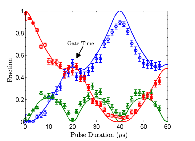
In more detail, the MS gate requires the simultaneous application of detuned blue and red sidebands. To achieve this, we overlap three laser beams with different frequencies in trap zone A (Fig. 2b (iii) ). One laser beam propagates along the co-carrier beam path with frequency . The other two beams co-propagate in the 90∘ beam path at frequencies of , where is the frequency of a motional mode and is a detuning. The two laser beams are derived from a single beam that is split and passed through different double-pass acousto-optic deflectors such that they end up with a frequency difference of . The split beams are then recombined on a - beam splitter with one port directed to the ions and the other going to a photo-detector that is used to measure and stabilize the phase of the beat note, as required to realize [25]. To implement , we simultaneously address the two highest-frequency axial motional modes for the four-ion crystal at and [32]. The detuning must be chosen such that the detuning from one mode is an integer multiple of the detuning from the other in order to fully disentangle both motional states from the qubit states at the end of the gate. Experimentally, we found a detuning of above was optimal given our laser beam intensities, which implies that the MS gate was implemented with one phase-space loop on the mode and four loops on the mode [22]. In Fig. 3 we plot the observed fraction of both ions in the state (red squares), both ions in the state (blue circles), and one ion in each state (green triangles) as a function of the duration of the red and blue sideband pulses applied to an initial state of . The MS gate is completed in approximately ().
For the Clifford and phase-gate benchmarks, we generated random sequences of lengths . The respective number of sequences implemented was for the Clifford benchmark, and for the phase-gate benchmark, in order of sequence length. Each time we performed a sequence for the Clifford benchmark we then immediately performed the corresponding phase-gate benchmark sequence. Each sequence was implemented times. From the measurement outcomes, we determined the fraction of measurements that matched the prediction. The data shown in Fig. 4 was obtained in four successive sets of experiments on the same day. During and between the sets we periodically recalibrated the magnetic field and the laser frequencies needed for sympathetic cooling of 24Mg but not the other pulse parameters. Within each set, the sequences were randomized with respect to length. However, the first (second, third, fourth) set involved sequences of lengths to (to , , , respectively). In particular, sequences of length were run only in the last set of experiments, which is why there are fewer sequences of length contributing to the data. During the experimental runs for these sets, we observed one ion-loss event. We did not implement longer sequences because ion-loss events became a problem for lengths greater than .
In our implementation, a Clifford unitary took on average. For the sequences with an extra gate inserted after each step, per step was typical. The most time-consuming elements of the sequence implementations were the sympathetic recooling of the ions after each recombination of the ions into trap zone A, followed by the separation and recombination processes. Each sequence began with approximately for state preparation and laser lock stabilization. Thus, a sequence of length with an extra inserted at each step lasted approximately . Longer sequences resulted in an accelerated rate of ion loss events (on the order of a loss event per minute), which can likely be attributed to a decreased probability of recovery from background gas collisions that can occur at any point during the sequences. Before running each sequence, two warmup sequences with experiments each were run to make sure the experiment was in a steady state; the results of these experiments were not recorded. Switching from one sequence to the next required to of computer time to reprogram the control hardware. In total, all of the Clifford benchmarks, including the sequences used to benchmark , were completed in approximately hour and minutes, which also includes the time durations needed for periodic recalibrations of the magnetic field as well as the time period to reload a set of ions following the only ion-loss event.
The parallel one-qubit benchmark whose results are shown in Fig. 5 was executed in one set, after all of the two-qubit benchmarks and following a recalibration of the one-qubit gates. The number of sequences implemented was for sequence lengths of , respectively. We ran each sequence times, as before. In order to approximately replicate the conditions of the experiment for the two-qubit benchmark, in each step, the ions were recombined into a single trap zone, recooled and then held for approximately the same duration required to execute before being separated again for the next sequence step.
IV Experimental Results
The red data points and curve in Fig. 4 show the results from the experimental Clifford gate benchmark and their match to an exponential decay. The match gives a Clifford unitary EPO of .

The blue data points and curve in Fig. 4 show the results from the benchmark. Curve-fitting and solving the above equations for give an EPG of .
We determined the errors per step on each qubit independently with the parallel one-qubit benchmarks explained above. The results from the benchmarks are shown in Fig. 5. The inferred one-qubit errors per step are and for the respective qubits. Using the assumption that laser pulses dominate the error per step, these results can be compared to the protocol of Ref. [5] through multiplication by the ratio of -pulses per step in the two protocols.

V Data Analysis Methods
In the limit of very large numbers of sequences for each length, we can use a simple, nonlinear, weighted-least-squares fit of Eq. (1) to the fidelity curves as a function of length. The weights are determined by the standard error of the mean for the fidelity at each length. Note that some non-linear least-squares fitting functions compute the error in the inferred parameters from the fitting error and ignore the scale of the errors implied by the weights given to the individual points. Because we already have a good estimate of the standard errors of these means, a better estimate of the error in the inferred parameters can be obtained by direct propagation of errors, particularly when there are few points.
For smaller numbers of sequences for each length, we must consider that we know little about the distribution of the fidelities for different random sequences of a given length. This distribution is affected not only by the differences in actual pulses applied, but also by factors such as the amount of coherence in error (see below). However, the estimate of a given sequence’s fidelity from the experimental runs is binomially distributed. Thus we used a partially parametric bootstrap [34] procedure to determine a standard error for the parameters inferred by fitting. Let be the number of different sequences of length used in the experiment. Denote the experimentally measured fidelity of the ’th sequence of length as , which is the fraction of times the correct result was obtained during the runs of the ’th sequence. We generated artificial data for each bootstrap resample as follows. For each length , we constructed by letting be a random element of the sequence of fidelities , picked independently (with replacement, that is, the same element can be picked multiple times) for different . For each , we generated a random according to a binomial distribution, so that was the fraction of ’s in random instances of a variable where the probability of was . We then averaged the for each length and computed the fit in the same way as it was computed for the real data to obtain the inferred parameters for this resample. This resampling procedure was repeated times, yielding resampled values for each of the parameters. The standard errors in the reported parameters are determined as the square-root of the variances of the corresponding resampled parameters. The values of the parameters are still the ones from the fit of the original experimental data, as this is the less biased estimate and requires no bootstrapping.
VI Consistency Checks
Although the relationship between EPOs and physical errors in gates is not known in general, specific benchmarking protocols provide well-defined EPOs that can be compared across platforms. However, for an implementation of the benchmark to be convincing, there are several assumed or expected properties that can be checked. These include the following: We can determine whether or not the fidelity curves are consistent with a simple exponential as a function of sequence length, and if not, analyze the deviations. Given that we know the implementations of the Clifford unitaries, we can compare the EPO for a Clifford unitary with that inferred from the EPG for a phase gate and the one-qubit benchmark.
First we consider the exponential fits shown in Fig. 4. The values (four degrees of freedom) for the two curves are and , respectively. The higher one corresponds to a -value of , approximately the conventional boundary for significance. There is other evidence that the exponential model may not be a good fit. First, the two preparation/measurement errors are expected to be the same, but the fits seem to suggest otherwise, although the statistical significance is not strong. Second, both sets of data seem to dip below the fit near the end. Together these observations suggest an increased EPO for later Clifford unitaries. Indeed, dropping the first points from the analysis suggests higher EPOs. For example, the fits for the last four and three sequence lengths have EPOs of and , respectively. The corresponding EPGs are and . Note that the second values are from a two-parameter fit to three points, which reduces their significance. The fits to the first four sequence lengths give an EPO of and an EPG of . The higher EPOs for longer sequences could be related to the fact that unlike the shorter ones, they were run only in the last or last two sets of experiments, without recalibrating pulse parameters except as noted above. We attempted to confirm this hypothesis by analyzing the results for sequence lengths one to three separately for each set. The results of this analysis are consistent with a drop but have insufficient signal-to-noise to be conclusive.
In principle, we would like the platform to have the property that errors reach stationary behavior soon after state preparation, and the benchmark’s reported EPO should reflect the stationary error. As noted above, we were not able to implement long enough or sufficiently many sequences to clearly observe stationary behavior, or to determine the extent to which the behavior is nonstationary. The EPO and EPG reported in the abstract are determined from all six lengths tested—given the “early” and “late” values above, we believe that they are a good representation of mid-length behavior of gate errors. Our inability to consistently run sequences of length longer than six prevents any claims of stationary behavior.
Other issues with the exponential fits that can arise include the possibility that the curves are a mixture of exponentials, as would be expected if the EPOs change slowly compared to the time required to run a sequence. In this case, the apparent EPOs would tend to decrease with increasing sequence length, as the higher-EPO runs affect the loss at shorter lengths, but tail behavior is dominated by the slowest decay. Given the observations of the previous paragraph and the available statistics, we cannot usefully test for this possibility.
Now we consider consistency between the measured EPOs and EPGs. We estimate the EPO that we should have measured given the EPGs obtained from the one-qubit and the phase gate benchmarks. For this estimate, we count the complexity of sequences of one-qubit pulses in terms of the number of effective -pulses applied. This counts only pulses around the or axes, taking into consideration that -axis pulses and identity gates are essentially error-free. The -pulses are counted as two -pulses. Coherent error addition is neglected. The one-qubit benchmark’s steps each have an average of effective -pulses per qubit. If we use as a representative error probability per step from the one-qubit benchmark (Fig. 5), we obtain as the linearized error probability per one-qubit -pulse. The factor of converts the average probability of error for one qubit to that for two qubits under the assumptions that the other qubit has no error and any Pauli error is twirled to a depolarizing error. For the purpose of this calculation, we take the error probability per phase gate to be . Each step in the Clifford benchmark has an average of effective pulses and phase gates. The linearized error probability for a step can therefore be estimated as , with a standard error of about , if we add the statistical errors in quadrature. This linear approximation is expected to give a pessimistic estimate, but in this case, the nonlinear correction is smaller than the error in the estimate. While our estimate gives a value below the measured EPO, the difference appears not to be statistically significant. We emphasize that the above strategy for estimating the EPO from EPGs neglects coherent error addition, which tends to increase the error, and internal error cancellation that could arise from the way pulses are combined within a step.
VII Estimates of Physical Sources of Error
We consider known sources of errors and estimate their contribution to the EPG of . Spontaneous emission is a fundamental source of error for transitions driven by stimulated-Raman transitions; here the laser beams are tuned approximately below the state [35, 36]. We simulate that for our laser parameters, this should contribute an error probability of to a one-qubit -pulse and to the phase gate. (Recall that the phase gate consists of an MS gate surrounded by -pulses.)
Errors can also arise from imperfect calibrations and slow drifts of the gate parameters. These parameters include beam intensities, frequencies, phases, and pulse durations. These types of errors are coherent in the sense that for any given run, each implemented gate still causes a unitary change in state, but not exactly the intended one. To determine whether such errors contribute significantly to the measured EPOs, we consider the variation in fidelities for different sequences of a given length. Coherent error contributions typically result in a variation that is larger than that expected from a simple statistical analysis [5]. For our experiment and in the absence of coherent errors, we attribute the largest sources of variation in the fidelities of Fig. 4 to the varying number of gates and single-qubit rotations needed to implement each step’s random Clifford unitary, and to the binomial statistics for the fidelities inferred from the runs of each sequence. Fig. 6 compares the actual variation and the variation predicted from the statistics of the number of phase gates per step and the binomial statistics. We did not include the variation in numbers of one-qubit gates due to their significantly smaller error. The gate statistics and binomial statistics are independent, so their contributions were added in quadrature. The predicted variation is generally somewhat less than the measured one but does not indicate coherence of the errors in a given sequence because our simple model does not account for all incoherent effects.
The main sources of coherent errors are due to drifts in beam intensity, relative laser field phases for the beams implementing the phase gate, and Stark-shifted frequencies. These drifts result in errors in pulse time, and phase and frequency calibration, each of which are estimated to contribute approximately equally to the EPG. We estimate that their total contribution to the phase gate EPG is less than .

There are a number of lesser sources of error to consider. In addition to the slow intensity drifts included above, there are also fluctuations in intensities that can be slow compared to sequence duration but are too fast to be calibrated out. For example, these can arise from fluctuations in laser power or from noise in the position of the laser beams with respect to the ions, due to vibration and air movement. Such fluctuations in intensity lead to loss of visibility in Rabi flopping curves [23, 5]. From such curves, we determined that the Rabi rate on the carrier transition with the non-copropagating beams fluctuates by from experiment to experiment. This results in a contribution of [18] to the phase gate EPG.
Due to the finite Lambe-Dicke parameter for the ions, fluctuations in ion motional energy can cause errors in the MS gate [23, 37]. As in Ref. [32], we estimate that each motional mode is cooled to an average excitation of at most quanta before the implementation of each phase gate. This leads to errors in the MS gate of due to the finite excitation of the modes directly involved in the gate and due to the fluctuating Debye-Waller factors of the other modes combined [23, 37].
Intrinsic background heating for the ions results in motional decoherence in the MS gate while the spins and motion of the ions are entangled. We measure a heating rate for a single 9Be+ ion to be to quanta per millisecond in the common axial mode at a confinement frequency of . However, the motional modes used for the MS gate have only a small component of the center-of-mass motion. Conditions here are essentially the same as those of a previous experiment [20], and imply a contribution of less than to the phase gate’s error.
To perform the phase gate, the optical path lengths of the two non-copropagating beams should ideally remain constant throughout the gate’s three-pulse sequence, whose duration is . Measurements of the optical beat-note between the non-copropagating Raman beams give a linewidth of order ; from this we estimate that optical-path-length fluctuations result in a phase-gate error of the order of , assuming the relative phase fluctuations at the beat-note detector are the same as those experienced by the ions.
The qubit coherence time and thus the benchmark error probabilities are affected by fluctuations in the magnetic field and its gradients, which cause differential frequency shifts in the qubits. Experimentally we determine a qubit coherence time by measuring the decay of the contrast in a two-pulse Ramsey experiment as a function of the duration between pulses. We find a coherence time of . Due to the resolution limit of our frequency synthesizer, which serves as a clock to keep track of the qubit phases during the randomized benchmarking experiments, we are systematically detuned from the qubit frequency by . The error due to this frequency offset should be negligible, given the typical time required for a Clifford unitary of a few milliseconds. We measure a magnetic field difference between trap zones A and B of , which leads to a systematic frequency difference between the qubits of a few millihertz depending on the exact value of the magnetic-field.
As an independent check on phase-gate fidelity, we measured the state fidelity for a Bell state created by use of the phase gate , as was done in Refs. [14, 15, 18]. Such measurements were performed before and after the randomized benchmarking data was taken. Before the benchmark we determined a Bell state fidelity of . After the benchmark we obtained . These fidelities include errors due to imperfect state initialization, detection, and three carrier -pulses using the co-propagating beams that are needed to prepare and analyze the state. A measurement of the state fidelity where the Bell state was prepared using only the MS gate and analyzed with a single non-copropagating carrier -pulse, thereby removing one non-copropagating carrier pulse and three co-propagating carrier pulses from the measurement, gave . The fidelities are consistent with the EPG determined by the benchmark.
Errors for one-qubit gates implemented with copropagating beams are likely dominated by changes in the Rabi rate [5]. An indication of whether or not long-term drifts may have affected the two-qubit benchmark can be obtained by comparing two one-qubit benchmarks. The first was run immediately after the two-qubit benchmark, without recalibrating. The second followed recalibration of the relevant pulses and is the one that we reported above. The first one found EPGs and for the two qubits, respectively, suggesting that at least the second qubit’s gates may have been in need of recalibration by the end of the two-qubit benchmarks.
Error can also be caused by loss of ions due to background gas collisions. We checked for loss of ions after each sequence, and if an ion-loss event was detected, we removed the previous sequence from the data set. We observed a significant increase in the rate of ion loss events for sequences involving more than ion separation/recombination processes—one such process is needed for each phase gate performed. This limited the maximum length of the sequences used in the randomized benchmarking. The reason for the increase in the rate of ion loss is not understood.
In summary, the errors discussed in the previous paragraphs amount to a phase gate EPG of about (linearized, incoherent error addition) to be compared to the benchmark-determined EPG of . The EPG estimate of includes for spontaneous emission, for calibration imperfections, for intensity fluctuations, for ion motion, for motional heating, and for optical path length fluctuations. The fact that our measured error is greater than our estimated error based on known physical sources suggests that our model of errors for the phase gate is incomplete.
VIII Multi-qubit Randomized Benchmarking
Clifford benchmarks as defined above can serve as a platform-independent strategy for comparing the quality of quantum operations in a computational context. For qubits, the expressions for the EPOs and EPGs of Eq. (1) and (4) are generalized as follows:
| (5) | |||||
| (6) |
where is a gate being characterized by insertion after each step. These equations can be established under idealizing assumptions in the same way as Eqs. 1 and 4, after observing that for qubits, the probability that the sequence does not depolarize is . The comparison on the basis of EPOs and EPGs obtained from the length-dependent loss of fidelity makes sense in the absence of significant deviations from the simple exponential-decay model. The thus-measured EPGs can be meaningfully interpreted as true average gate errors in the idealized case where the errors are independent, depolarizing and stationary. In general, the connection to the actual error-behavior of elementary gates is not well understood [9]. Nevertheless, we believe that sufficiently small randomized-benchmark-determined EPGs are a good indication of gate quality that can be compared to a general-purpose fault-tolerance threshold goal such as the often-mentioned . In the above, we have considered how to take into account the indications for non-exponential decay in our data. Generally, if there is clear evidence of non-exponential decay, the behavior and range of observed EPOs and EPGs and the extent to which stationary behavior was achieved need to be discussed. Given sufficiently many sequence lengths, these ranges can be determined by considering different-length intervals. Initial transients in error behavior may be expected even in the case where stationary behavior is achieved for longer sequences and can be analyzed separately.
The translation of a given Clifford unitary into a circuit of elementary gates suitable for a given platform is up to the experimenter, so some improvements are possible by greater efficiency of the translation rather than higher quality gates. We consider such “software” improvements to be potentially as useful as strictly “hardware”-based ones. Furthermore they are usually easier for others to implement. However, we believe that for small numbers of qubits, such circuit translations are already sufficiently close to optimal for software improvements of this sort to be self-limiting. The individual gate benchmarks implemented by inserting specific gates after the Clifford unitaries can show directly how much the gate quality has improved, independent of how the Clifford unitaries have been translated into circuits of elementary gates.
When benchmarking qubits, we suggest that the benchmarks are applied to different subsets of the qubits so that comparable EPOs are obtained for qubits. We recommend that such benchmarks be applied in parallel to disjoint subsets, if possible. This solves the problem of comparing new results to earlier ones involving platforms with fewer qubits. Nevertheless, it would be helpful to have a way of comparing EPOs for the Clifford benchmark that is independent of the number of qubits. One possibility is to divide the EPO by , the average over Clifford unitaries of the minimum number of controlled-not gates needed to implement them with a circuit consisting of controlled-not gates and arbitrary one-qubit Clifford gates. For two qubits, this normalization factor is determined by , so the normalized Clifford EPO for our benchmark is . For three qubits we determined rounded at the last digit. Since the number of Clifford unitaries grows very rapidly with , it may be difficult to determine the normalization factor exactly for . It is known that scales as [38, 27, 28]. While this complexity may seem relatively large at first, any viable platform must be able to implement circuits of this size, if not much larger. In particular, any successful demonstration of the Clifford benchmark also establishes the ability to implement non-trivial circuits for algorithmic purposes.
If the primary purpose of the experiment is to benchmark individual gates by inserting them after randomized unitaries, it is desirable to find ways to achieve sufficient randomization that are more efficient than random Clifford unitaries. In particular, to exhibit an EPG of a gate in this way, it suffices for the random unitaries to approximate a so-called unitary -design as explained in [1]. Such approximations are possible with circuits involving a logarithmic multiple of two-qubit gates [1]. How to best translate these theoretical ideas into a practical benchmark remains to be determined.
For the Clifford benchmark, the strategy for choosing the final unitary of a sequence given above is more constrained than necessary for ensuring that the measurement outcome is deterministic in the absence of error. This may result in less effective error depolarization. We suggest two alternatives that greatly reduce the constraints on . The first is to choose uniformly at random from all Clifford unitaries that ensure that the final state in the absence of error is a logical state. This is equivalent to constructing as an implementation of the inverse of the previous unitaries followed by a random gate that can be decomposed into CNOT and Pauli product operators. An even more randomizing approach is to choose as suggested in Ref. [5]. In this case, is composed of a uniformly random Clifford unitary followed by one-qubit Clifford gates randomly chosen to ensure that a randomly chosen joint -measurement is deterministic in the absence of errors. By a joint -measurement we mean measurement of a product of operators on a subset of the qubits. The product’s eigenvalues are and can be determined by multiplying the standard basis measurement outcomes of the qubits in the subset, where a qubit’s and measurement outcomes are mapped to , , respectively. This strategy takes advantage of the often much better fidelity of one-qubit gates for the sequence-dependent part of the last unitary. A disadvantage is that instead of deterministic bit values, only one bit value is obtained in each run of the experiment. To fit the resulting data, we use Eqs. 5 and 6 with .
IX Conclusion
In summary, we have described a protocol for randomized benchmarking of gates in a quantum information processor and implemented the protocol experimentally on two qubits to measure the error per operation of arbitrary two-qubit Clifford unitaries. The protocol we propose is independent of the gate set that is experimentally implemented and so can provide an easily portable method for evaluating the performance of Clifford unitaries on different physical platforms. Furthermore, with this method it is straightforward to isolate the fidelity of a specific two-qubit gate. We have emphasized some of the consistency checks that can be performed to qualify the reported errors per operation or gate. Looking ahead, this randomized benchmarking protocol should prove useful as different experimental implementations of quantum information processors aim to increase the number of qubits and work to decrease the errors towards what is required for fault-tolerance.
Acknowledgements.
This work was supported by NSA, IARPA, ONR and the NIST Quantum Information Program. The authors would like to thank Scott Glancy and Brian Sawyer for careful readings of the manuscript. JPG is supported by NIST through an NRC fellowship. This paper is a contribution by NIST and not subject to U.S. copyright.References
- [1] C. Dankert, R. Cleve, J. Emerson, and E. Livine, Phys. Rev. A 80, 012304 (2009), arXiv:quant-ph/0606161.
- [2] J. Preskill, Proc. R. Soc. Lond. A 454, 385 (1998).
- [3] E. Knill, Nature 463, 441 (2010).
- [4] T. D. Ladd, F. Jelezko, R. Laflamme, Y. Nakamura, C. Monroe, and J. L. O/’Brien, Nature 464, 45 (2010).
- [5] E. Knill, D. Leibfried, R. Reichle, J. Britton, R. B. Blakestad, J. D. Jost, C. Langer, R. Ozeri, S. Seidelin, and D. J. Wineland, Phys. Rev. A 77, 012307 (2008).
- [6] C. A. Ryan, M. Laforest, and R. Laflamme, New Journal of Physics 11, 013034 (2009).
- [7] I. L. Chuang and M. A. Nielsen, J. Mod. Opt. 44, 2455 (1997).
- [8] J. Poyatos, J. Cirac, and P. Zoller, Phys. Rev. Lett. 78, 390 (1997).
- [9] E. Magesan, J. M. Gambetta, and J. Emerson, arXiv:1109.6887 (unpublished).
- [10] K. R. Brown, A. C. Wilson, Y. Colombe, C. Ospelkaus, A. M. Meier, E. Knill, D. Leibfried, and D. J. Wineland, Phys. Rev. A 84, 030303(R) (2011), arXiv:1104.2552.
- [11] J. M. Chow, J. M. Gambetta, L. Tornberg, J. Koch, L. S. Bishop, A. A. Houck, B. R. Johnson, L. Frunzio, S. M. Girvin, and R. J. Schoelkopf, Phys. Rev. Lett. 102, 090502 (2009).
- [12] J. M. Chow, L. DiCarlo, J. M. Gambetta, F. Motzoi, L. Frunzio, S. M. Girvin, and R. J. Schoelkopf, Phys. Rev. A 82, 040305(R) (2010).
- [13] S. Olmschenk, R. Chicireanu, and J. V. Porto, New Journal of Physics 12, 113007 (2010).
- [14] C. A. Sackett, D. Kielpinski, B. E. King, C. Langer, V. Meyer, C. J. Myatt, M. Rowe, Q. A. Turchette, W. M. Itano, D. J. Wineland, and C. Monroe, Nature 404, 256 (2000).
- [15] D. Leibfried, B. DeMarco, V. Meyer, D. Lucas, M. Barrett, J. Britton, W. M. Itano, B. Jelenković, C. Langer, T. Rosenband, and D. J. Wineland, Nature 422, 412 (2003).
- [16] P. C. Haljan, P. J. Lee, K.-A. Brickman, M. Acton, L. Deslauriers, and C. Monroe, Phys. Rev. A 72, 062316 (2005).
- [17] J. P. Home, M. J. McDonnell, D. M. Lucas, G. Imreh, B. C. Keitch, D. J. Szwer, N. R. Thomas, S. C. Webster, D. N. Stacey, and A. M. Steane, New Journal of Physics 8, 188 (2006).
- [18] J. Benhelm, G. Kirchmair, C. F. Roos, and R. Blatt, Nat Phys 4, 463 (2008).
- [19] M. Riebe, K. Kim, P. Schindler, T. Monz, P. O. Schmidt, T. K. Körber, W. Hänsel, H. Häffner, C. F. Roos, and t. . P. T. o. I. T. Q. G. R. Blatt”, Phys. Rev. Lett. 97, 220407/1 (2006).
- [20] J. P. Home, D. Hanneke, J. D. Jost, J. M. Amini, D. Leibfried, and D. J. Wineland, Science 325, 1227 (2009).
- [21] J. D. Jost, Ph.D. thesis, Univ. of Colorado, Boulder, Boulder, CO, 2010.
- [22] A. Sørensen and K. Mølmer, Phys. Rev. Lett. 82, 1971 (1999).
- [23] D. J. Wineland, C. Monroe, W. M. Itano, D. Leibfried, B. E. King, and D. M. Meekof, J. Res. Natl. Inst. Stand. Technol. 103, 259 (1998).
- [24] D. Kielpinski, C. Monroe, and D. J. Wineland, Nature 417, 709 (2002).
- [25] P. J. Lee, K.-A. Brickman, L. Deslauriers, P. C. Haljan, L.-M. Duan, and C. Monroe, J. Opt. B 7, S371 (2005).
- [26] D. Gottesman, in Proceedings of Symposia in Applied Mathematics, edited by J. Samuel J. Lomonaco (American Mathematical Society, Washington, DC, 2010), Vol. 68, pp. 13–58, arXiv:0904.2557.
- [27] S. Aaronson and D. Gottesman, Phys. Rev. A 70, 052328 (2004).
- [28] K. N. Patel, I. L. Markov, and J. P. Hayes, Quantum Information and Computation 8, 0282 (2008).
- [29] D. Gottesman, Ph.D. thesis, Calif. Inst. Tech, Pasadena, California, 1997, quant-ph/9705052.
- [30] M. A. Nielsen and I. L. Chuang, Quantum Computation and Quantum Information (Cambridge University Press, Cambridge, UK, 2001).
- [31] A. R. Calderbank, E. M. Rains, P. W. Shor, and N. J. A. Sloane, IEEE Trans. Inf. Th. 44, 1369 (1998).
- [32] J. D. Jost, J. P. Home, J. M. Amini, D. Hanneke, R. Ozeri, C. Langer, J. J. Bollinger, D. Leibfried, and D. J. Wineland, Nature 459, 683 (2009).
- [33] D. Hanneke, J. P. Home, J. D. Jost, J. M. Amini, D. Leibfried, and D. J. Wineland, Nature Physics 6, 13 (2010).
- [34] B. Efron and R. J. Tibshirani, An Introduction to the Bootstrap (Chapman & Hall, New York, 1993).
- [35] R. Ozeri, W. M. Itano, R. B. Blakestad, J. Britton, J. Chiaverini, J. D. Jost, C. Langer, D. Leibfried, R. Reichle, S. Seidelin, J. H. Wesenberg, and D. J. Wineland, Phys. Rev. A 75, 042329 (2007).
- [36] H. Uys, M. J. Biercuk, A. P. VanDevender, C. Ospelkaus, D. Meiser, R. Ozeri, and J. J. Bollinger, Phys. Rev. Lett. 105, 200401 (2010).
- [37] A. Sørensen and K. Mølmer, Phys. Rev. A 62, 022311 (2000).
- [38] V. V. Shende, A. D. Prasad, I. L. Markov, and J. P. Hayes, IEEE Transactions on Computer-Aided Design of Integrated Circuits and Systems 22, 710 (2003).