Which point sets admit a $k$-angulation?⁰⁰footnotetext: This research was supported by the DAAD and the Go8 within the Australia–Germany Joint Research Co-operation Scheme 2011 as part of the project Problems in geometric graph theory (Kennz. 50753217).

Since $G$ is $2$-connected the boundary of the outer face is a cycle $C$; say it has $r$ vertices. $P$ has at least $n-r$ interior points since every internal vertex must be an interior point. Let $e$ be the number of edges and $f$ be the number of faces in $G$. Thus $2e=k(f-1)+r$. Euler’s formula states that $n-e+f=2$. Thus, $n-r=n-2e+k(f-1)=n-2(n+f-2)+k(f-1)=k-n+(f-2)(k-2)$. Hence $n-r\equiv_{k-2}k-n$. Since $n-r$ is non-negative, $P$ contains at least $j$ interior points. ∎

Since $G^{\prime}$ is $2$-connected, all its faces are bounded by simple cycles. It remains to show that the internal faces are bounded by $k$-cycles. Each internal face of $G^{\prime}$ corresponds to a block with $k-2$ vertices in $G^{*}$. If a block contains a cycle, then the boundary of the corresponding face is not connected. Therefore, every block is a tree. Thus the number of edges in every block is $k-3$. This implies that the number of edges in the boundary of every internal face is $3(k-2)-2(k-3)=k$. ∎

Let $B$ be an inclusion maximal bad convex path in $C$. By definition, $z$ is contained strictly inside the convex hull of $\bar{B}$. Thus, $\bar{B}$ covers an angle of more than $\pi$ at $z$. Since $B$ is maximal convex, any other maximal bad convex path must be disjoint from $\bar{B}$, but this would exceed the total angle $2\pi$ at $z$. ∎

If $j=0$, then $n\equiv_{k-2}k$. There exists an outerplanar $k$-angulation with $f$ faces for every $f$, and the number of vertices is $k+(f-2)(k-2)\equiv_{k-2}k$. Therefore, using the result of Gritzmann et al. [14] mentioned above, a $k$-angulation can be drawn on $P$.

If $j>0$ then there is at least one interior point. Select an arbitrary interior point $z$ and construct the wheel triangulation with $z$ as the central vertex. If $j=1$ then the number of triangles in the wheel triangulation is $n-1\equiv_{k-2}k-j-1=k-2$. The weak dual is a cycle on $n-1=c(k-2)$ vertices, where $c\geq 2$ since $n\geq 2k^{2}$. This cycle can be partitioned into $c$ blocks, each of which is a path of order $k-2$. The subgraph of the wheel triangulation corresponding to this block partition is a subdivision of a wheel graph with $c$ spokes, and is therefore $2$-connected. Hence, by Proposition 3, it is a $k$-angulation.

Now assume $2\leq j\leq k-3$. We start by using Algorithm 1 to add $m:=j-1$ triangles to the wheel triangulation. Note that $m$ is the number of triangles we must add to the $n-1$ triangles of the wheel triangulation to make the total number of triangles a multiple of $k-2$. As triangles are added, the current outer cycle is denoted $C^{\prime}$. Reflex and non-reflex vertices on $C^{\prime}$ are defined analogously to those on $C$. Each time a triangle is added, a reflex vertex of $C^{\prime}$ becomes an internal vertex. In this way, we may identify each triangle with a unique vertex, and each triangulation (which extends the wheel triangulation) with a sequence of vertices.

Algorithm 1 is initialised at a non-reflex vertex on $C^{\prime}:=C$. Moreover, if there is a maximal bad convex path $B$, it is initialised at a non-reflex vertex inside $B$. It then proceeds clockwise around $C^{\prime}$ (see Figure 3). Each time it encounters a reflex vertex of $C^{\prime}$, it adds a triangle there, proceeds to the next vertex clockwise around $C^{\prime}$, and then updates $C^{\prime}$. Algorithm 1 stops when it has added $m$ triangles. The output is the sequence $S:=(s_{1},\dots,s_{m})$ of vertices in $C$ where triangles were added.

Algorithm 1 may complete many laps around $C^{\prime}$. If at some time no more triangles can be added, then $C^{\prime}$ must be a convex polygon. In this case, all interior points of $P$ have been removed from $C^{\prime}$, so at least $m$ triangles have been added. Therefore Algorithm 1 always terminates.

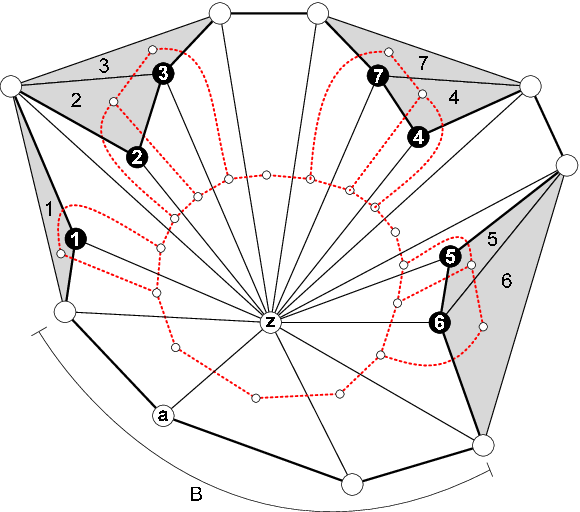
Let $G_{t}$ be the triangulation and $G^{*}_{t}$ the weak dual after Algorithm 1 has added $t$ triangles.

Recall that $S$ is the set of vertices in $C$ on which Algorithm 1 added triangles. Consider the collection of paths induced by $S$ in $C$. Each such path contains a reflex vertex of $C$, otherwise it would be a convex path and no triangle could be added on it. Therefore, for every convex path $X$, $X\setminus S$ is a single path.

Let $L$ be the subgraph induced in $C$ by the set of vertices that are visited by Algorithm 1. $L$ is either a path or all of $C$. An original reflex vertex of $C$ remains a reflex vertex of $C^{\prime}$, unless it is added to $S$. So Algorithm 1 never passes over a reflex vertex of $C$ without adding it to $S$. Therefore, even if $S$ does not contain all the reflex vertices of $C$, there must exist a path in $L$ that

(1) contains every vertex in $S$,

(2) contains no reflex vertices in $C\setminus S$ and

(3) does not intersect the path $B\setminus S$ (if a maximal bad convex path $B$ exists).

Let $U$ be the longest path in $C\setminus S$. Thus

We distinguish the following cases.

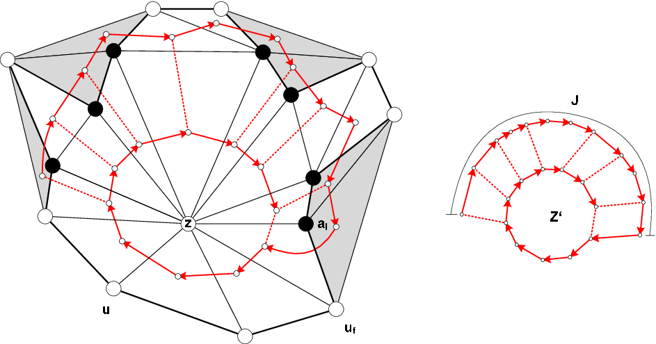
Case 1: All triangles added by Algorithm 1 share an edge with $C$.

$G^{*}$ contains a Hamiltonian path $H$ that begins at the start of $J$, then traverses $J$ and passes from the last vertex of $J$ to the inner cycle $Z^{\prime}$, visiting the rest of the vertices in clockwise order. We call this a spiral path. Since $|G^{*}|=n-1+m\equiv_{k-2}0$, the path $H$ can be partitioned into blocks consisting of paths each with $k-2$ vertices.

We now show that the subgraph of $G$ corresponding to this block partition of $G^{*}$ is $2$-connected, and hence a $k$-angulation of $P$ by Proposition 3. In the wheel triangulation, all vertices in the outer cycle $C$ are neighbours of $z$. In the final triangulation $G$ there are two large cycles, the new outer cycle $C^{\prime}$, and the cycle through the neighbours of $z$, call it $C_{z}$. Within $A$, the addition of triangles over the vertices of $S$ removes them from $C^{\prime}$, while pontoons are built over $A\setminus S$, removing these vertices from $C_{z}$. The vertices in $P\setminus(A\cup\{z\})$ make up²² 2 Since the endpoints of $A$ are in $S$, $U$ is maximal in $C\setminus S$, and $U$ is not contained in $A$, it follows that $U$ is the complement of $A\cup\{z\}$. $U$ and remain in both $C^{\prime}$ and $C_{z}$. Hence these two cycles intersect in the path $U$, which has order at least $2k$.

Now consider the subgraph $G^{\prime}$ of $G$ corresponding to the block partition described above. Since $U$ has order at least $2k$, there is at least one edge left from $z$ to a vertex $u$ in $U$. There is also an edge from $z$ to the clockwise last point $a_{l}$ in $A$, where the last block in $H$ ends. All edges of the cycles $C^{\prime}$ and $C_{z}$ remain except for possibly the edge from $a_{l}$ to the first vertex $u_{f}$ in $U$. Therefore, there is a $2$-connected spanning subgraph of $G^{\prime}$ consisting of the union of $C^{\prime}$, $C_{z}-a_{l}u_{f}$ and the path $a_{l}zu$. This subgraph is a $\theta$-graph (that is, a graph consisting of two vertices joined by three internally disjoint paths).

The weak dual graph $G^{*}$ now consists of the inner cycle $Z^{\prime}$, and the remaining outer section $J:=G^{*}-Z^{\prime}$. As before, the triangles of the pontoons form paths connecting the paths induced by the $m$ added triangles. However this time $J$ consists of two separate paths because the pontoon $R$ does not cover all of $U$ and $C\setminus A$ is not empty. Let $J_{1}$ be the path containing $R$, and let $J_{2}$ be the second path.

We now describe two disjoint paths that together cover all the vertices of $G^{*}$. The first path $H_{1}$ begins at the clockwise first vertex in $R$, traverses $J_{1}$ then passes to $Z^{\prime}$, continues clockwise until it can pass to the clockwise first vertex of $J_{2}$ and then continues to the end of $J_{2}$. Note that augmenting the pontoon $R$ by one triangle moves a vertex from $Z^{\prime}$ to $J_{1}$ and therefore enlarges $H_{1}$ by one vertex. Since $|U|>2k$, we can choose the order of $R$ such that the number of vertices in $H_{1}$ is a multiple of $k-2$ and still leave at least $k$ vertices in $Z^{\prime}$. The remaining vertices form a second path $H_{2}$ that is contained in $Z^{\prime}$. Since the total number of vertices in $G^{*}$ is a multiple of $k-2$, the order of $H_{2}$ must also be a multiple of $k-2$. Thus, both paths can be partitioned into blocks.

We again show that the subgraph $G^{\prime}$ of $G$ corresponding to this block partition of $G^{*}$ is $2$-connected, and hence a $k$-angulation of $P$ by Proposition 3. The outer cycle $C^{\prime}$ is a simple cycle. The internal vertices all lie on the boundary between the blocks of $H_{1}$ and the blocks of $H_{2}$. This boundary forms a path $D$ starting at the clockwise last vertex $u$ of $U$ that is not covered by the pontoon $R$, then proceeding clockwise through the neighbours of $z$ to the last vertex $a_{l}$ of $A$, then passing to $z$, then to the first vertex $a_{f}$ of $A$, and then proceeding clockwise through the neighbours of $z$ until the first vertex $u_{f}$ of $U$. Thus $C^{\prime}\cup D$ forms a spanning subgraph of $G^{\prime}$ which is again a $\theta$-graph.

Case 2: Some triangle added by Algorithm 1 shares no edge with $C$.

Before giving the full details, we sketch the remainder of the proof. We will begin by building pontoons between the trees $\{T_{i}\}$. Our goal is to partition the trees and pontoons into blocks separately from the inner cycle. Difficulties may arise from the fact that (unlike the paths in Case $1$) trees cannot in general be split into two components of arbitrary size. To avoid this problem, we will require that each tree is contained in a block (recall that no tree is larger than a block). This is possible if there are enough choices for where to start the first block. To this end, we build an additional pontoon at the start of the outer section of the weak dual. The order of this pontoon is chosen so that no block starts inside a tree.

We now give a detailed account of this method.

The weak dual $G^{*}$ now consists of two sections, the inner cycle $Z^{\prime}$ and the connected subgraph $J:=G^{*}-Z^{\prime}$ consisting of the trees and the pontoons (see Figure 6). The vertices of the trees have an ordering given by the clockwise order of their corresponding vertices in $A$, and the vertices of the pontoons have a clockwise ordering in $J$. Let $\sigma$ be a linear ordering of the vertices of $J$ that is consistent with these orderings, and where the intervals corresponding to each tree and pontoon are concatenated in the order they appear in $J$. That is, $\sigma$ begins with the vertices of $R$, then continues with the vertices of the first tree, then the next pontoon, then the second tree, and so on.

The partition of $G^{*}$ into blocks is done in a spiral manner similar to Case $1(a)$, starting with $J$ then passing to $Z^{\prime}$. $J$ is partitioned according to $\sigma$, taking the first $k-2$ vertices, then the next $k-2$ and so on. The order of the initial pontoon $R$ may be between $0$ and $k-3$. Adjusting the order of $R$ shifts the blocks in $\sigma$, and each order determines a set of block starting points. These sets partition $\sigma\setminus R$. A block must not start inside a tree (though it may start at the first vertex of a tree), so there are less than $m$ places in $\sigma$ where a block may not start. Since $m<k-2$, there must be some set of block starting points that avoids these obstructions. This implies that there exists a feasible order for $R$ such that all trees lie inside a block.

Just as in Case $1(a)$, we now show that there is a $2$-connected spanning subgraph of the graph $G^{\prime}$ corresponding to this block partition. Again there are two cycles $C^{\prime}$ and $C_{z}$, but in this case their intersection is not the whole of $U$, but rather just the part of $U$ not covered by $R$. Nevertheless, this remainder has order greater than $k$, so there is again an edge left from $z$ to a vertex $u$ inside it. There is also an edge from $z$ to $a_{l}$, the clockwise last vertex of $A$. All edges of $C^{\prime}$, and all but one of $C_{z}$ remain, and again there is a spanning $\theta$-subgraph consisting of these edges and the path $a_{l}zu$. Hence, by Proposition 3, $G^{\prime}$ is a $k$-angulation.

The partition of $G^{*}$ into blocks has two sections (similar to the two paths in Case $1(b)$). The first section starts at the first vertex of $R$, traverses $J_{1}$ according to the ordering $\sigma_{1}$, then passes to $Z^{\prime}$, continuing clockwise until it can pass to the first vertex of $J_{2}$, then continues according to the ordering $\sigma_{2}$ to the last vertex of $L$. The order of $R$ is chosen so that no block ends inside a tree. Then the order of $L$ is chosen so that the total number of vertices in this section is divisible by $k-2$. The second section of the partition is the remainder of $Z^{\prime}$. Since $|U|>2k$, and building each of $L$ and $R$ removes at most $k-3$ vertices, there are at least $6$ vertices of $U$ not covered by $L$ and $R$. This implies that the remainder of $Z^{\prime}$ is non-empty, and thus contains at least one block.

Just as in Case $1(b)$, we now show that there is a $2$-connected spanning subgraph of the graph $G^{\prime}$ corresponding to this block partition. As before, it consists of the outer cycle $C^{\prime}$ and a path $D$ covering the internal vertices. $D$ starts at the clockwise last vertex $u$ of $U$ that is not covered by the pontoon $R$, then proceeds clockwise through the neighbours of $z$ to the last vertex $a_{l}$ of $A$, then passes to $z$, then to the first vertex $a_{f}$ of $A$, and then proceeds clockwise through the neighbours of $z$ until the first vertex $u^{\prime}$ of $U$ that is not covered by the pontoon $L$. Thus $C^{\prime}\cup D$ forms a spanning $\theta$-subgraph of $G^{\prime}$, so $G^{\prime}$ is a $k$-angulation by Proposition 3. This concludes the proof of Theorem 1. ∎

The proof of Theorem 1 describes the algorithm. Here we outline the complexity of the main steps. The first step is to compute the convex hull boundary of $P$, a task that can be done in $O(n\log n)$ time using standard methods (see for example [7]). If there are less than $j$ interior points the algorithm terminates here and reports that no $k$-angulation exists (by Proposition 2).

The case $j=0$ requires drawing an outerplanar $k$-angulation on $P$. If we select an outerplanar $k$-angulation whose dual is a path, Bose [2] gives an $O(n\log n)$ time algorithm to do this. For $j\geq 1$, constructing the wheel triangulation, which requires sorting the points radially about $z$, can be done in $O(n\log n)$ time. The case $j=1$ is finished after the edges are removed from the initial triangulation to make a $k$-angulation; this takes $O(n)$ time.

For $j\geq 2$, we go through the major steps used in Algorithm 1 and in the construction of the $k$-angulation. Whether an external vertex is reflex can be determined in $O(1)$ time. Thus, a bad convex path $B$ can be computed in $O(n)$ time. In certain examples, Algorithm 1 may find as few as one triangle to add per lap around $C$, so the number of steps is $O(kn)$. Having determined the set $S$, the paths $A$ and $U$, and thus the case distinction, can be calculated in $O(n)$ time.

Building a pontoon of order $p$ takes $O(p)$ time, so the pontoons joining parts of $S$ can be built in $O(n)$ time. The dual graph can also be constructed with standard methods in $O(n)$ time. Computing the order of a pontoon such that the last block of the partition contains exactly $k-2$ vertices can be done in $O(n)$ time. In Cases $2(a)$ and $2(b)$, we need to compute the order of a pontoon $R$ such that all resulting blocks have valid starting points, that is, starting points that are not inside a tree. The order of $R$ may be between $0$ and $k-3$. In these cases, we simply iterate through each of the $k-2$ possibilities and check if all the resulting blocks have valid starting points. This takes $O(kn)$ time. The partition of the dual graph into blocks can be computed by traversing the dual graph in the manner described in $O(n)$ time. Finally, removing the edges to form a $k$-angulation takes $O(n)$ time. In total, we get a running time of $O(kn+n\log n)$. ∎

References

- [1] T. Biedl and M. Vatshelle. The point-set embeddability problem for plane graphs. Tech. Report CS-2011-27, University of Waterloo, Canada, November 2011.
- [2] P. Bose. On embedding an outer-planar graph in a point set. Comput. Geom. Theory Appl., 23(3):303–312, 2002.
- [3] P. Bose and G. Toussaint. No quadrangulation is extremely odd. In Algorithms and Computations, volume 1004 of Lecture Notes in Computer Science, pages 372–381. Springer, 1995.
- [4] P. Bose and G. Toussaint. Characterizing and efficiently computing quadrangulations of planar point sets. Computer Aided Geometric Design, 14(8):763–785, 1997.
- [5] S. Cabello. Planar embeddability of the vertices of a graph using a fixed point set is NP-hard. J. Graph Algorithms Appl., 10(2):353–363 (electronic), 2006.
- [6] N. Castañeda and J. Urrutia. Straight line embeddings of planar graphs on point sets. In Proc. Eighth Canadian Conference on Computational Geometry, pages 312–318, 1996.
- [7] M. de Berg, O. Cheong, M. van Kreveld, and M. Overmars. Computational geometry. Springer-Verlag, Berlin, third edition, 2008. Algorithms and applications.
- [8] T. K. Dey, M. B. Dillencourt, S. K. Ghosh, and J. M. Cahill. Triangulating with high connectivity. Comput. Geom. Theory Appl., 8(1):39–56, 1997.
- [9] E. Di Giacomo, W. Didimo, G. Liotta, H. Meijer, F. Trotta, and S. K. Wismath. -colored point-set embeddability of outerplanar graphs. J. Graph Algorithms Appl., 12(1):29–49, 2008.
- [10] E. Di Giacomo, W. Didimo, G. Liotta, H. Meijer, and S. K. Wismath. Constrained point-set embeddability of planar graphs. Internat. J. Comput. Geom. Appl., 20(5):577–600, 2010.
- [11] E. Di Giacomo, W. Didimo, G. Liotta, and S. K. Wismath. Book embeddability of series-parallel digraphs. Algorithmica, 45(4):531–547, 2006.
- [12] E. Di Giacomo, G. Liotta, and F. Trotta. Drawing colored graphs with constrained vertex positions and few bends per edge. Algorithmica, 57(4):796–818, 2010.
- [13] A. García, F. Hurtado, C. Huemer, J. Tejel, and P. Valtr. On triconnected and cubic plane graphs on given point sets. Comput. Geom. Theory Appl., 42:913–922, 2009.
- [14] P. Gritzmann, B. Mohar, J. Pach, and R. Pollack. Problems and Solutions: Solutions of Elementary Problems: E3341. Amer. Math. Monthly, 98(2):165–166, 1991.
- [15] J. M. Schmidt and P. Valtr. Cubic plane graphs on a given point set. In Proceedings of the 28th Annual Symposium on Computational Geometry (SoCG’12), to appear (2012).
- [16] C. Thomassen. Kuratowski’s theorem. Journal of Graph Theory, 5(3):225–241, 1981.
- [17] G. Toussaint. Quadrangulations of planar sets. In Algorithms and Data Structures, volume 955 of Lecture Notes in Comput. Sci., pages 218–227. Springer, Berlin, 1995.