Multiple Membranes in M-theory
Abstract
We review developments in the theory of multiple, parallel membranes in M-theory. After discussing the inherent difficulties with constructing a maximally supersymmetric lagrangian with the appropriate field content and symmetries, we introduce 3-algebras and show how they allow for such a description. Different choices of 3-algebras lead to distinct classes of 2+1 dimensional theories with varying degrees of supersymmetry. We then demonstrate that these theories are equivalent to conventional superconformal Chern-Simons gauge theories at level , but with bifundamental matter. Analysing the physical properties of these theories leads to the identification of a certain subclass of models with configurations of M2-branes on orbifolds. These models give rise to a whole new gauge/gravity duality in the form of an correspondence. We also discuss mass deformations, higher derivative corrections, and the possibility of extracting information about M5-brane physics.
Keywords:
String theory, M-theory, BranesCERN-PH-TH-2012-94
RUNHETC-2012-05
TIFR/TH/12-06
NI-12-013
1 M-theory and M-branes: a brief review
M-theory is a proposed interacting quantum theory involving fields and extended objects (“branes”) propagating in 11 spacetime dimensions. Its existence has been inferred from the properties of its massless fields, including the spacetime metric, which couple to each other via a specific classical lagrangian known as “11d supergravity,” to be described in more detail below. In addition to the massless fields, M-theory possesses two kinds of stable branes, namely 2-branes (equivalently referred to as “membranes”), and 5-branes. These are dynamical objects that extend in two and five spatial dimensions respectively (as well as time) and possess a characteristic tension and charge.
11d supergravity [1] is a locally supersymmetric lagrangian field theory involving massless bosons and fermions. It is special in that eleven is the highest spacetime dimension in which a consistent supersymmetric theory can be written down that has spins [2]. The theory has one 32-component spinor supercharge in eleven dimensions and, if we allow no more than two-derivative interactions, its lagrangian is unique. However, given the non-renormalisability of gravity in any dimension greater than or equal to four, it is not obvious how to extend this lagrangian to an ultraviolet-complete quantum theory. For this reason, the role of the 11d supergravity lagrangian in quantum physics remained unclear for many years.
The situation for supergravity theories in 10 spacetime dimensions is superficially similar. Type II supergravities have two spacetime supersymmetry charges, which in turn singles out ten as the maximum allowed spacetime dimension. With only two-derivative interactions and this amount of supersymmetry there is not one unique lagrangian, but rather two possible lagrangians with different field contents. These are referred to as type IIA and type IIB supergravity. Again, because of non-renormalisability, these lagrangians by themselves do not define an ultraviolet-complete quantum theory.
However, in these cases, an ultraviolet completion is known. Type IIA and IIB supergravities are the low-energy limits of corresponding superstring theories. In particular, this is how type IIB supergravity was originally discovered [3] and subsequently constructed [4, 5]. As shown in Ref. [3], there are two superstring theories in 10 dimensions, type IIA and IIB. Quantisation of these strings reveals, in particular, a spectrum of massless particles. Computations of string scattering amplitudes for these modes can be used to read off their low-energy lagrangians, and the resulting theories are type IIA and type IIB supergravity.11 1 Type IIA supergravity also arises by compactifying 11d supergravity on a circle [6, 7, 8], as we will discuss in more detail later. This fact, together with considerable evidence that string theory is ultraviolet finite, encourages us to think of superstring theory as the ultraviolet completion of type II supergravity. The full theory includes not just the massless modes of supergravity but also extended objects, specifically strings. It was later understood that the spectrum also includes extended branes. These have been studied from a variety of complementary points of view: in terms of worldvolume field theories of the degrees of freedom bound to them, as charged extended soliton-like solutions in supergravity, and as one-dimensional matrix models.
This relation between superstring theory and 10d supergravity provides a basis to conjecture the existence of a theory that similarly completes 11d supergravity in the ultraviolet (UV). Indeed, it was long expected that fundamental membranes play a role analogous to the one that strings play in completing ten-dimensional supergravities (see for example Refs.[9, 10]). This idea was further stimulated by the discovery that when compactifying 11d supergravity, wrapped membranes naturally turn into the fundamental strings of type IIA superstring theory [11]. While it has not actually proved possible to quantise fundamental membranes and derive 11d supergravity from them, it was argued via duality [12, 13, 14] that there is a consistent UV completion of 11d supergravity and that stable membranes are an important part of this theory.
The details of this conjectured theory, called “M-theory,” will be described below. In addition, for previous reviews on M-theory, its duality properties, compactifications, as well as complementary aspects of membrane dynamics, we refer the reader to [15, 16, 17, 18, 19, 20]. As we will see, 11d supergravity has no scalar fields and no dimensionless couplings. Therefore in particular it has no tunable coupling constant. The same must therefore be true of the hypothetical M-theory whose low-energy action is postulated to be 11d supergravity. It follows that unlike string theory, M-theory has no perturbative expansion. This makes it considerably harder to study than string theory. We believe in the existence of M-theory only because of many different properties and relationships that have been uncovered in the last three decades. These together provide convincing evidence for the existence of an elegant and internally consistent structure. In this chapter and the next, we will attempt to exhibit this structure. A key feature will be the presence of supersymmetric membranes and 5-branes.
The fact that 10d type IIA supergravity arises by dimensional reduction of 11d supergravity strongly suggests that the ultraviolet completions of the two theories (explicitly known in the former case and conjectural in the latter) are related. Indeed it has been convincingly argued [12, 13, 14] that upon starting with type IIA string theory and allowing the string coupling to become very strong, the resulting theory reveals a hidden eleventh dimension and should be thought of as M-theory. Conversely, upon compactifying the underlying eleven-dimensional spacetime on a spatial circle, M-theory reduces to type IIA string theory with the string coupling being related to the radius of the circle. This comparison is more subtle and rich than comparison of merely the low-energy effective actions. Indeed, here one keeps the Kaluza-Klein states [7] arising on compactification, as well as states arising from wrapped or unwrapped branes, and (as we explain below) a perfect match ensues. Thus M-theory is in fact a limit of string theory: more precisely, a novel and unexpected description of the dynamics of string theory in a strong-coupling region where the familiar string formalism (specifically perturbation theory) is not applicable.
A major puzzle in M-theory has been to understand which, if any, of its degrees of freedom plays a “fundamental” role analogous to that of the fundamental string in string theory. This is at least partially answered [11] by noticing that when M-theory turns into type IIA string theory upon compactifying a spatial dimension, the membrane of M-theory wrapped on this dimension can be identified with the fundamental string. In this sense the membrane appears to be the most fundamental object in M-theory, providing renewed justification for earlier attempts to treat it thus. Indeed it is presumably the origin of the letter “M” in “M-theory.” One must however be very careful about this interpretation because while quantisation and scattering are well-understood (perturbatively) for the fundamental string, there is no simple analogue for the membrane in M-theory.
A key feature of modern string theory is the dynamics of multiple D-branes [21], which are described by the end points of open strings. This description provides a great deal of insight into the worldvolume dynamics of the branes, which is described by familiar classes of gauge theories augmented by higher-derivative corrections. It should not come as a surprise that the dynamics of multiple membranes (and also of multiple 5-branes) is more complex than that of multiple D-branes. In parallel with our limited understanding of everything else about M-theory, relatively little has been known about the degrees of freedom localised on membranes and 5-branes. In the last few years, however, considerable progress has been made in understanding the interacting field theory on multiple membranes in M-theory. This constitutes the subject of the present review.
We note that there have been various attempts to directly define an eleven-dimensional quantum theory of gravity involving membranes. The first, well before the name M-theory was coined, aimed to quantise membranes as one does for strings. However this was later found to be fraught with difficulties (see e.g. [22]). A later definition involved reducing the degrees of freedom to those of matrices living on the worldvolume of D0-branes in the so-called infinite momentum frame [23]. That both of these approaches involve fundamental degrees of freedom that begin with the letter “M” is surely one of the reasons for the current name: M-theory. There is a great deal of literature concerning a single, quantum, membrane in eleven-dimensional supergravity; for example see the pioneering works [24, 25]. This review cannot claim to do justice to this topic; rather we aim to give a review of recent results concerning the infrared quantum description of multiple M2-branes in terms of novel highly supersymmetric gauge theories, analogous to the role of Yang-Mills gauge theories on D-branes.
In the remaining part of this chapter we provide a pedagogical discussion of 11d supergravity and its relationship to type IIA supergravity in 10d, along with a survey of the stable branes of M-theory. For the latter, we start in historical order with their worldvolume descriptions and go on to describe their appearance as stable classical solutions of 11d supergravity. We then show how M-theory and type IIA string theory branes are related.
The rest of this review is organised as follows. In Chapter 2 we make precise the definition of multiple membrane field theory and discuss the Basu-Harvey proposal, involving a triple-bracket, for the structure of such a theory. We also review the basics of supersymmetric Chern-Simons theories which are the foundation on which multiple membrane theories are built. In Chapter 3 we develop the mathematical structure of superconformal Chern-Simons field theories based on “3-algebras.” This includes the construction of the Bagger-Lambert-Gustavsson (BLG) model, which was the first example of a maximally supersymmetric lagrangian that was not a Yang-Mills theory, and the first description of multiple (albeit only two) M2-branes. All these developments come together in Chapter 4 where the Aharony-Bergman-Jafferis-Maldacena (ABJM) action, the effective description for multiple membranes in M-theory placed at an orbifold singularity, is presented. In Chapter 5 we begin the analysis of various features of the ABJM theory, including its relation to super-Yang-Mills via the novel Higgs mechanism as well as its connection to the BLG models. In Chapter 6 we continue with some more advanced topics, covering the description of M-theory momentum by monopole operators, as well as an extension of the theory through a mass deformation and its subsequent spacetime interpretation in terms of dielectric membranes. In Chapter 7 we consider more general superconformal Chern-Simons theories with reduced supersymmetry () and give their 3-algebra description. In Chapter 8 a few other potentially interesting directions are presented where 3-algebra-based theories play a role, including Lorentzian 3-algebras, higher derivative corrections and applications to M5-branes. Some closing remarks are presented in Chapter 9. For a less technical review, the reader is referred to [26].
1.1 Eleven-dimensional supergravity
A massless field with spin equal to 2 in four dimensions (and its analogues in higher dimensions) can be consistently coupled in a field theory only if the couplings obey general coordinate invariance. The spin-2 field is then identified with the metric of spacetime and upon quantisation becomes a “graviton,” the mediator of the gravitational force. Moreover, interacting massless fields with spin greater than 2 are believed to be inconsistent unless there are infinitely many of them. Therefore in trying to construct a supergravity theory we should look for a supermultiplet of bosonic and fermionic fields for which the highest spin is 2.
Indeed, just assuming supersymmetry and a spin-2 field one deduces that the supersymmetry must be local in spacetime. This arises from the fact that the anticommutator of two supersymmetries is a translation generator – in gravity, translations are promoted to local (general coordinate) transformations and the supersymmetry generators accordingly must generate transformations that are local in spacetime. Theories of this sort are called “supergravities.”
The metric or graviton field is denoted with . In spacetime dimensions this has on-shell degrees of freedom. This counting comes from the fact that the little group is , and the on-shell graviton transforms in the symmetric traceless representation of this group.
Supersymmetry requires that there be a superpartner for the graviton, known as the “gravitino” . The gravitino is the gauge particle of local supersymmetry (just as a Yang-Mills field is the gauge particle of usual gauge invariance). It is a fermion with both a vector and a spinor index, . Here is the dimension of the irreducible spinor representation of the little group, which depends in a complicated way on . The gravitino has on-shell degrees of freedom. To see this, note that a simple spinor of components has components on-shell while a -component vector has components on-shell. Thus a gravitino apparently has degrees of freedom. However due to the well-known properties of -matrices the “-trace” of the gravitino field, defined as , is clearly an irreducible representation by itself. Therefore to get an irreducible representation one must remove this part by imposing “-tracelessness”
| (1.1.1) |
which subtracts on-shell degrees of freedom, leaving the number quoted above.
To find a supermultiplet one can now compare the number of physical degrees of freedom of a graviton and a gravitino and try to account for the difference – if any – by introducing additional fields. We look for supermultiplets with the minimal amount of supersymmetry in a given dimension. From the discussion above, it follows that there will be a single gravitino. We exhibit the degrees-of-freedom count for various spacetime dimensions in the following table
| Spacetime dimension | Spinor dimension | Graviton | Gravitino | Difference |
| 4 | 4 | 2 | 2 | 0 |
| 5 | 8 | 5 | 8 | 3 |
| 6 | 8 | 9 | 12 | 3 |
| 7 | 16 | 14 | 32 | 18 |
| 8 | 16 | 20 | 40 | 20 |
| 9 | 16 | 27 | 48 | 21 |
| 10 | 16 | 35 | 56 | 21 |
| 11 | 32 | 44 | 128 | 84 |
| 12 | 64 | 54 | 288 | 234 |
The deficit can be made up by adding new bosons to the theory. However, once we reach there are so many bosons needed that we inevitably encounter “spin ” fields (we have not proved this here but it is the content of a theorem to which we referred earlier). For , we need to add bosonic fields with 84 on-shell degrees of freedom to obtain a matching of on-shell degrees of freedom, a necessary condition for supersymmetry. Fortunately there is an irreducible representation of the little group that has precisely this dimension. It is the antisymmetric 3-form . In general this has on-shell degrees of freedom, and for this is precisely 84!
Thus we may hope to find an 11d supergravity theory containing the massless fields
| (1.1.2) |
Indeed, it was shown by Cremmer, Julia and Scherk [1] that the following action is supersymmetric
| (1.1.3) | |||||
Here, is the Newton constant in 11 dimensions. It has dimensions of [length]9 and is often written in terms of , the 11d Planck length, via
| (1.1.4) |
The other quantities appearing in the above action are defined as follows. is the Ricci scalar and is the covariant derivative
| (1.1.5) |
The spin connections and are defined in terms of the vielbein (defined by ) and the gravitino as
| (1.1.6) |
with being the usual Levi-Civita spin connection associated to . has the property of being supercovariant – its supersymmetry variation does not contain derivatives of the supersymmetry parameter. Finally, the field strengths and are defined as
| (1.1.7) |
In form notation and
| (1.1.8) |
The supersymmetry transformations, labelled by an arbitrary spacetime-dependent infinitesimal spinor parameter , are as follows
| (1.1.9) |
where the antisymmetrised gamma-matrices are defined as22 2 The action and supersymmetry transformations given above follow from those of Ref. [1] by rescaling and such that a common factor of appears in front of all terms, and then sending , , , , to convert from the “mostly minus” metric there to the “mostly plus” one used in the present review. .
The above action is general-coordinate-invariant (and actually, since it involves fermions, also local-Lorentz-invariant), as one would expect of any action involving gravity. Additionally it is invariant up to a total derivative under the “2-form gauge symmetry”
| (1.1.10) |
where is an arbitrary infinitesimal spacetime-dependent 2-form.
1.2 Relation to string theory
So far we have not exhibited any relationship between M-theory and string theory. A relationship between them is strongly suggested by the compactification of 11d supergravity to 10 dimensions. For this, we assume the eleventh dimension is compactified on a circle with periodicity and find the massless fields in ten dimensions by taking the eleven-dimensional fields to be independent of . We must also decompose tensors and spinors into irreducible representations of the ten-dimensional Lorentz algebra. This is part of the process called Kaluza-Klein reduction (which additionally involves massive fields in the lower dimension arising from non-constant modes over the compact space).33 3 For a review of Kaluza-Klein supergravity see [27].
Let us now use the indices to denote 10d spacetime indices and for 10d tangent-space indices. Then the 11d metric and 3-form reduce as follows [7, 8, 13]
| (1.2.1) |
The quantities on the right hand side of the equalities are all ten-dimensional (both in the sense that they are representations of the 10d Lorentz group and that they depend on the 10d coordinates). This has not been denoted explicitly by a label except where confusion may occur.44 4 Note that is a scalar field. The decomposition above anticipates that an exponential parametrisation for the scalar will be natural.
The decomposition of the metric in the first line was chosen in part so that, using the standard identity for block matrix determinants
| (1.2.2) |
we have
| (1.2.3) |
The curvature term of the 11d action then reduces as
| (1.2.4) |
Similarly the 3-form-dependent terms of the 11d action reduce as
| (1.2.5) |
where we are being schematic and have omitted terms that involve powers of . We notice that the bosonic fields of the dimensionally reduced theory, that is a metric , a scalar and a 1-form, 2-form and 3-form (we drop the superscript from now on), are in one-to-one correspondence with the fields of type IIA supergravity in 10 dimensions. The latter has a metric, a scalar called the dilaton and a 2-form , all coming from the Neveu-Schwarz-Neveu-Schwarz sector, and 1-form and 3-form Ramond-Ramond potentials and .
The bosonic part of the type IIA supergravity action is
| (1.2.6) | |||||
where is the “string length” associated to type IIA string theory, of which this 10d supergravity is the low-energy limit.
To match the two sides we may perform a Weyl transformation on the metric and also a rescaling of . However we are not allowed to absorb powers of in the gauge potentials as these will lead to derivative couplings with the dilaton which are not present in type IIA supergravity in the frame in which we are working. It is now easy to see that with
| (1.2.7) |
the two actions match perfectly up to the overall constants in front of the integrals.
To match these constants, we first note that the 10d and 11d Planck lengths are related by virtue of the relation between 10d and 11d metrics
| (1.2.8) |
This tells us that a given physical distance , when measured in units of , is related to the same distance as measured in units of by
| (1.2.9) |
From the dilaton dependence of the type IIA action above we can read off that the constant part or VEV of the dilaton defines the string coupling via
| (1.2.10) |
It follows that
| (1.2.11) |
With this identification, we can match the coefficients if we set
| (1.2.12) |
where on the RHS we have extracted the VEV of from the integral. Substituting Eq. (1.2.11) in Eq. (1.2.12) we immediately find
| (1.2.13) |
To summarise, we have seen in this section that 11d supergravity, when compactified on a circle to 10d, is identical to type IIA supergravity. There is a definite relationship between the Planck lengths of the two theories, and also between the radius of compactification of the 11d theory (a parameter absent in the 10d description) and the coupling constant of the 10d theory (absent in the 11d description). At small radius or weak coupling the type IIA description is more appropriate, while at large radius or strong coupling it is the 11d description that is more appropriate. As we remarked earlier, since type IIA supergravity in 10d has a consistent ultraviolet completion in the form of type IIA string theory, this strongly suggests that 11d supergravity also has a consistent UV completion, which corresponds to the strongly coupled limit of type IIA string theory. It is this hypothetical completion that bears the name “M-theory.”
1.3 Motivations to study extended objects
There are two distinct kinds of limitations in our understanding of M-theory. One is that we have formulated it in a fixed spacetime background55 5 While here we have only chosen flat Minkowski spacetime, many other noncompact and partially compactified backgrounds are known and have been investigated. and it is not clear how to study M-theory in a background-independent way. Of course an analogous problem holds also in the existing formalisms of string theory. The other limitation is that there is no direct way to prove the existence of a consistent ultraviolet completion of 11d supergravity. In contrast, it can be quite convincingly demonstrated using the string perturbation expansion that superstring theories in 10 dimensions are ultraviolet finite, so at least in perturbation theory we can be sure they provide consistent UV completions of their low-energy supergravity theories. This cannot be repeated in M-theory due to the absence of a coupling constant.
However, given that in string theory it is the string size that cuts off possible ultraviolet infinities, one might suspect that something similar holds in M-theory, namely that it is a theory of not just point particles but also extended objects, one or more of which somehow provides an ultraviolet cutoff. This provides an important motivation to study extended objects or branes in 11d supergravity, to which we turn our attention in the following section.
Another related motivation to study extended objects in 11d supergravity is that the spectrum of type IIA string theory contains, besides the fundamental string, a profusion of other stable supersymmetric extended objects. The latter include both Dirichlet branes (“D-branes”) that exhibit unusual and striking features, as well as other more conventional branes. If the relationship that we have discussed above between 11d supergravity and type IIA supergravity in 10d lifts to a relationship between the hypothetical M-theory and the UV-complete type IIA string theory, there must be a precise relationship between the stable branes in the two theories. With this motivation in mind we construct branes of M-theory in the next section from two points of view: as extended worldvolume field theories and as soliton-like extended solutions of classical 11d supergravity. Then we go on to discuss their relationship with branes of type IIA string theory in 10d. As the title of this review indicates, the M-theory brane that will be of greatest interest to us is the 2-brane or membrane.
1.4 Worldvolume actions for M-theory branes
Worldvolume actions for particles or extended objects determine (after quantisation) the quantum mechanical behaviour of these objects. Typically they are made up of kinetic terms and couplings to gauge fields under which the object is charged. For M-branes, the worldvolume action crucially includes couplings to the 3-form gauge field.
To understand the origin of such couplings, recall the well-known coupling of a particle to a gauge field , which is
| (1.4.1) |
integrated along the worldline of a particle. The worldline itself is given by some function where is a parameter. Then the above coupling can be better written as
| (1.4.2) |
where
| (1.4.3) |
is the “pull-back” of the gauge field onto the worldline of the particle.
In string theory we encounter a generalisation of this where the particle worldline is replaced by the string worldsheet where labels points along the string. The analogous coupling of the string is to a 2-form field
| (1.4.4) |
where and
| (1.4.5) |
is the pull-back of the -field to the string worldsheet.
In general, the rank of the gauge potential is related to the spatial dimension of the charged object by . In the examples above, we see that point particles () are electrically charged under 1-form potentials, as is familiar in electromagnetism, while strings () are “electrically” charged under 2-forms. Now as long as all dimensions are noncompact, the only gauge field in 11d supergravity is the 3-form . It follows that the only possible electrically charged objects in this theory are 2-branes, or membranes, whose charge is manifested via the worldvolume coupling
| (1.4.6) |
Here are the worldvolume coordinates, with the first one being worldvolume time and the last two labelling points on the membrane, while
| (1.4.7) |
is the pull-back of the -field to the 2-brane worldvolume.
While the above must be a term in the 2-brane action in M-theory, it cannot of course be the whole story. As mentioned above we need to add kinetic terms. In addition, as we will explain later, the stable 2-branes in M-theory are actually supersymmetric. Therefore we have to supersymmetrise the worldvolume action.
We first present the bosonic part of the M2-brane action. It contains 11 scalar fields representing the brane coordinates, and a worldvolume metric that is treated as an independent field. The 11d supergravity fields and are treated as fixed backgrounds and the action is [9]
| (1.4.8) |
This is rather similar to the well-known action for a string worldsheet. Note however that while the worldvolume metric decouples for that case (in the critical dimension), here it remains a dynamical degree of freedom. Moreover the cosmological term in the worldvolume metric sets it equal, via the equations of motion, to the pull-back of the spacetime metric onto the brane
| (1.4.9) |
Supersymmetrising this action is most effectively done in superspace. To avoid going into all the complexities of the superspace construction, we restrict ourselves at present to a flat target spacetime, with vanishing 3-form , which will provide sufficient insight. In this case, the superspace action is easily reduced to an action for the bosonic coordinates and a set of fermionic coordinates . The latter are spinors in spacetime and scalars on the brane worldvolume. Although the number of bosonic and fermionic coordinates is not equal, we will soon see that both of them are effectively reduced to 8 degrees of freedom thanks to various symmetries. The discussion that follows is based largely on Ref. [28].
Let us define the quantity
| (1.4.10) |
The supersymmetric M2-brane action in flat spacetime with a vanishing 3-form gauge field is then
| (1.4.11) | |||||
Note that even though the background 3-form has been set to zero, the last term in the above action resembles a 3-form coupling – in particular, it is independent of the worldvolume metric and therefore topological. Indeed, it arises from a 3-form coupling in superspace.
The symmetries of this action under spacetime translations and Lorentz transformations, as well as under local worldvolume reparametrisations, are manifest. That leaves the fermionic symmetries, which are of two types. One is a rigid supersymmetry transformation with a constant parameter , which is a spacetime spinor and a worldvolume scalar. This transformation is
| (1.4.12) |
We see that the worldvolume metric is neutral under this rigid spacetime supersymmetry. The other is a local fermionic symmetry, called -symmetry, with an arbitrary worldvolume coordinate-dependent parameter that, like , is a spacetime spinor and worldvolume scalar. The worldvolume metric transforms non-trivially under the -symmetry transformations. It is convenient to define the quantities
| (1.4.13) |
The -symmetry transformations are then given by66 6 We assume the membrane is closed and has no boundary.
| (1.4.14) | |||||
We will return shortly to the question of gauge-fixing this local symmetry. It is useful to note at this stage that the -symmetry variation of , defined in Eq. (1.4.10), vanishes. As a consequence all the quantities in Eq. (1.4.13) are -invariant.77 7 The factors of cancel out against implicit powers in the symbol.
Let us now examine the equations of motion following from the action Eq. (1.4.11). As already indicated above in a bosonic context, the equation of motion for the worldvolume metric sets it equal to the pull-back of the spacetime metric. In the present case the spacetime is flat but since we are dealing with a supersymmetric theory, we find from Eq. (1.4.10) that the pull-back is implemented via the super-covariant quantity
| (1.4.15) |
This equation ensures the useful relations
| (1.4.16) |
The equation of motion for the bosonic coordinates is
| (1.4.17) |
while the equation for the fermionic coordinates is found to be
| (1.4.18) |
The latter equation can be rewritten, using both relations in Eq. (1.4.16), as
| (1.4.19) |
Note that both the above equations are invariant under the rigid supersymmetry transformations as given in Eq. (1.4.12).
Using the equations of motion we can finally analyse the on-shell degrees of freedom of the super-membrane. The reason we have given names to the LHS of the above equations is that it becomes easy to display three relations among them
| (1.4.20) |
Since these equations involve only the canonical momenta of the bosonic coordinates , without any time derivatives of the momenta, they are not dynamical evolution equations. Instead, they amount to constraints. In this way the 11 bosonic coordinates are reduced to 8 independent coordinates.
For the fermions, we started with which has 32 components. By virtue of the last equation of Eq. (1.4.16), acts like a gamma-matrix and therefore Eq. (1.4.19) is like a Dirac equation. However it differs from a conventional Dirac equation by having the projection operator in front. Indeed this is what ensures -symmetry, which acts by a shift in preceded by the orthogonal projector (the remaining quantities are already -invariant as we have noted.) This allows us to remove half the degrees of freedom of . The Dirac equation then has its usual effect of halving the remaining degrees of freedom, so at the end we are left with 8 on-shell fermionic coordinates. The matching of on-shell Bose and Fermi degrees of freedom is a necessary condition for supersymmetry.
To extract the physical degrees of freedom one must choose a suitable gauge that fixes worldvolume reparametrisations and -symmetry. A convenient choice is static gauge, in which we choose the time and two arbitrary spatial directions in the target spacetime and identify them with the worldvolume coordinates. Thus, we first carry out a split and re-labelling
| (1.4.21) |
and then impose the gauge-fixing conditions
| (1.4.22) |
For our purposes it is sufficient to assume this has been done locally. Whether these conditions can be imposed globally will depend on the topology of the membrane.
Once the static gauge has been chosen, we must re-examine the symmetries of the theory. Those which violate the gauge condition will, clearly, no longer be symmetries of the gauge-fixed theory. However some linear combinations of them may preserve the gauge and these will be genuine symmetries. An example of this is the combination of general coordinate transformations on the worldvolume (which can be represented infinitesimally as local worldvolume translations) and spacetime Lorentz symmetry
| (1.4.23) |
Choosing , we see that each of these terms separately violates the gauge condition. However performing both transformations together on , we get
| (1.4.24) |
This variation vanishes for the special choice
| (1.4.25) |
It follows that the gauge-fixed theory will be invariant under those combinations of worldvolume translations and spacetime Lorentz transformations that satisfy Eq. (1.4.25) above, namely
| (1.4.26) |
The first term on the right-hand-side corresponds to a worldvolume Lorentz transformation for a set of scalars . To see this, note that under
| (1.4.27) |
where is the parameter of worldvolume Lorentz transformations, a worldvolume scalar changes by
| (1.4.28) |
This tells us that is to be identified with and the subgroup of the spacetime Lorentz group is thereby identified with the worldvolume Lorentz group.
The last term on the RHS of Eq. (1.4.26) shows that the are vectors under rigid rotations of the spacetime transverse to the membrane worldvolume, generated by the parameters . Finally, the second term on the RHS of Eq. (1.4.26) is a non-linear transformation that parametrises the coset .
The same combination of worldvolume general coordinate transformations and spacetime Lorentz transformations on the fermionic coordinate (which is a spacetime spinor and worldvolume scalar) becomes, in the static gauge
| (1.4.29) |
where we have written only those terms that depend on the parameters. The first two terms in Eq. (1.4.29) give the transformation laws of a worldvolume spinor, while the last term is the transformation law of a spacetime spinor under transverse rotations in spacetime.
We have only gauge-fixed the worldvolume reparametrisations. It still remains to fix the local -symmetry on the worldvolume. This may be achieved by imposing
| (1.4.30) |
where
| (1.4.31) |
This projects to a chiral spinor with respect to . In what follows we will assume the above steps have been carried out and the fermionic coordinate is re-labelled corresponding to a set of 8 real two-component worldvolume spinors transforming in the spinor of .
In parallel with the case of bosonic symmetries discussed above, we now find that the (rigid) spacetime supersymmetry transformations are not by themselves invariances of the gauge-fixed action, but must be accompanied by a compensating -symmetry transformation as in Eq. (1.4.14). One can easily show that the static-gauge theory has maximal or global supersymmetry in 2+1 dimensions.
From here on we will always work in static gauge. The bosonic part of the action is
| (1.4.32) |
where , and on the right hand side we have dropped a constant and restored the precise dependence on the 11d Planck length , as well as constant factors. We see that the action is an expansion in powers of derivatives, where the leading term is simply the free kinetic term for 8 worldvolume scalars .
The number 8 coincides with the number of spatial directions transverse to the M2-brane. This is no coincidence but can be derived by noticing that in the presence of a 2-brane, spatial translational invariance of the bulk theory is broken from ten independent translations to only two (those along the brane). The eight broken translations correspond to the directions transverse to the brane. From the worldvolume point of view these appear as spontaneously broken symmetries, and we therefore expect – and find – an equal number of massless Goldstone bosons – the scalar fields .
The above action (after incorporating the fermion terms) represents a single M2-brane. The question now is to understand what should be the action for multiple M2-branes. This is an interesting problem even at lowest-derivative order, and is the main subject of this review. Before addressing it directly, we continue by reviewing a different approach to M2-branes, wherein they are seen as stable supersymmetric soliton solutions of the bulk 11d supergravity.
1.5 M-branes as solitons
In this section we display the stable brane solutions of 11d supergravity. Their stability will be guaranteed by supersymmetry through a result of Witten and Olive [29], who showed that for charged configurations in supersymmetric theories, the charge in appropriate units typically provides an exact quantum-mechanical lower bound on their mass (or tension, for extended objects). This bound was originally discovered (in a classical, non-supersymmetric context) by Bogomolny, Prasad and Sommerfield [30, 31] and is known as the BPS bound. The simplest BPS branes preserve half of the 32 spacetime supersymmetries of the supergravity theory. In addition to guaranteeing stability, this property will provide a relatively simple method to discover the brane solutions.
In what follows it will be convenient to use the eleven-dimensional “Planck length” , as defined in (1.1.4). The condition for a background to preserve supersymmetry is that there should exist some nonzero spinor or spinors such that the supersymmetry variations on the given background vanish. Since we only consider bosonic backgrounds (the fermions are set to zero), the supersymmetry variations of the bosons vanish identically. Thus we only have to check the supersymmetry variations of the fermions. Then the requirement for a supersymmetric solution is
| (1.5.1) |
where we have dropped the hats on and because the fermionic terms have been set to zero. Being first order, these equations are much easier to solve than the full second-order equations of motion. Moreover, because of supersymmetry, the corresponding configurations still satisfy the EOM.
Charged solutions carry the flux of some (generalised) gauge field. The only possible flux in uncompactified 11d supergravity comes from the 3-form , whose field strength is the 4-form defined above. The spatial components of this 4-form, , are analogous to a magnetic field while the components with one time and three space indices, , are analogous to an electric field. Accordingly, classical solutions will be labelled “electric” or “magnetic” depending on which of these fluxes they involve. The electric field is conveniently studied by dualising it to a 7-form
| (1.5.2) |
and then retaining the spatial components of this 7-form. The contribution ensures that on shell, in the presence of the Chern-Simons term.
Let us first find the magnetically charged classical solution. As discussed above, this will have a nontrivial flux . The magnetic charge will be . Here is a 4-sphere that encloses the charged object. This in turn tells us the dimensionality of the object, for in spacetime dimensions (equivalently spatial dimensions), a -sphere encloses a dimensional object.88 8 In 3 space dimensions this is familiar as the fact that a 2-sphere encloses a point, and a circle encloses an infinitely extended string. Since we are now considering a 4-sphere in 11 dimensions, the above formula tells us that the charged object must extend along dimensions. Therefore this is a 5-brane, henceforth referred to as the -brane [32].
By a similar argument involving spatial components of the 7-form flux defined above, we conclude that an electrically charged object in dimensions must extend along dimensions. This is therefore a 2-brane, called the -brane or membrane. In this case we will have a nonzero value of the electric charge where is a 7-sphere enclosing the M2-brane [33].
There can be more general objects carrying both types of charges [34, 35, 36]. These would be interpreted as bound states of M2- and M5-branes. They will turn out to preserve less supersymmetry than the individual planar M2- and M5-branes. Note that in uncompactified dimensions there are no other gauge fields and therefore no other types of charges available. As a result we do not expect to find any other stable, charged solitonic objects in the theory. In particular, there are no stable strings, which is further evidence that 11d supergravity is not the low-energy limit of a string theory.
1.6 The M2 and M5-brane tension
Let us now describe the M2-brane solution in some detail [33]. We take the coordinates along the brane to be while the coordinates transverse to the brane are denoted99 9 Here are just coordinates and not functions of , which is why we denote them by lower-case letters. . A planar 2-brane will have a symmetry corresponding to Lorentz transformations within the brane worldvolume and rotations of the space transverse to the brane. We also expect to have translational invariance along the brane, i.e. in the -coordinates.
These symmetries determine the M2-brane metric and electric flux to be of the form
| (1.6.1) |
where is the radial distance from the brane
| (1.6.2) |
and are functions of that need to be determined.
Imposing the equations of motion of 11d supergravity on the above ansatz, one finds that the three functions , and are all determined by a single function
| (1.6.3) |
where is a constant and is harmonic in the eight transverse dimensions: . In terms of this function we have
| (1.6.4) |
We can evaluate the total charge of the solution by integrating the appropriate flux. Using Eq. (1.5.2) and inserting the solution for specified in Eqs. (1.6.1), (1.6.4) we find the dual 7-form flux to be
| (1.6.5) |
In spherical polar coordinates with , has components only in the angular directions and can be written
| (1.6.6) |
from which it follows that the electric charge of the M2-brane is
| (1.6.7) |
with being the volume of a unit 7-sphere.
By comparing the metric with Newton’s law in the weak-field approximation, we can obtain a relation between the parameter in the solution and the tension of an M2-brane. The basic formula relates the time-time component of a static -brane metric in spacetime dimensions to the brane tension. For static, pointlike sources, Einstein’s equations in spacetime dimensions
| (1.6.8) |
reduce to
| (1.6.9) |
Using to leading order in the Newtonian approximation, one gets
| (1.6.10) |
Comparing this with Newton’s equation
| (1.6.11) |
we identify
| (1.6.12) |
For a pointlike source with , one has
| (1.6.13) |
and therefore
| (1.6.14) |
Since we assumed the source to be pointlike, this formula describes the Newtonian limit for black holes in arbitrary spacetime dimensions. It is easily generalised to extended black -branes. In this case, we label the coordinates of which the subset lie along the brane. For a static brane configuration and hence Eq. (1.6.9) is modified to
| (1.6.15) |
and therefore
| (1.6.16) |
Moreover, Eq. (1.6.13) changes to
| (1.6.17) |
where is the tension of the -brane, with dimensions of (mass)p+1. Combining these two results, we have
| (1.6.18) |
Applying this formula to M2-branes in 11 dimensions and comparing with Eq. (1.6.1) we find
| (1.6.19) |
where is the number of 2-branes and is the tension of a single M2-brane. Using Eq. (1.1.4) we then obtain
| (1.6.20) |
For the M5-brane [32], we take the coordinates on the brane to be , and the coordinates transverse to the brane to be . By reasoning similar to the M2-brane case, we assume a symmetry and also translational invariance in the -coordinates. These symmetries fix the metric to be of the form
| (1.6.21) |
Here is the radial distance from the 5-brane
| (1.6.22) |
Thus we need to find the functions and , and as before these are determined by a single function
| (1.6.23) |
where is a constant (that will be related to the magnetic charge of the 5-brane), and is harmonic in the 5 transverse dimensions: . In terms of this function we have
| (1.6.24) |
Additionally the magnetic flux of the solution is
| (1.6.25) |
The magnetic charge of the solution is
| (1.6.26) |
where is the volume of a unit 4-sphere.
Finally, using the Newtonian approximation once more, we find the relation
| (1.6.27) |
where is an integer, the number of M5-branes.
Since M-theory has only one dimensional parameter , we can predict on dimensional grounds that
| (1.6.28) |
Additional information on the actual values can be obtained using the Dirac quantisation condition, which tells us that
| (1.6.29) |
where is an integer [37]. Choosing single branes and the minimum quantum, i.e. , and making use of Eqs. (1.6.7), (1.6.20), (1.6.26), (1.6.27) we find
| (1.6.30) |
Setting the RHS equal to (because of the Dirac quantization condition), we find
| (1.6.31) |
In the next section, we will argue that the correct answers are
| (1.6.32) |
In the above solitonic description of branes it follows, using the techniques of soliton physics, that the translation symmetries broken by the brane are collective coordinates. Therefore the brane worldvolume will support a corresponding number of massless scalar fields. The M2-brane theory should then have 8 massless scalars, which we have already encountered in a previous section, while the M5-brane theory should have 5 massless scalars.
1.7 Relation to branes in string theory
If M-theory exists, the brane solitons we have found must be among its stable quantum excitations. The relation to string theory suggested in the previous section then tells us that after compactifying on a circle, the M-theory branes must reduce to one of the branes in type IIA string theory [13, 12, 14, 38]. Indeed one should be able to account for all stable branes in type IIA string theory from the M-theory perspective. This is potentially a challenge, since type IIA string theory has stable BPS D0, D2, D4 and D6-branes,1010 10 It also has D8-branes but, being domain walls, these change the nature of the spacetime and render the low-energy theory massive. It has recently been argued [39] that massive type IIA theory does not have a strong-coupling, weakly curved limit. as well as the fundamental string and the NS5-brane, while M-theory only has M2 and M5-branes. At the same time, we have already reproduced all the massless -form gauge fields under which the branes of type IIA string theory are charged; this provides a hint that things should work out properly.
Recall that BPS D-branes in type II string theory have tensions
| (1.7.1) |
In addition, there is a stable string (the fundamental string) and its electric dual, the NS5-brane. The formulae for their tensions are as follows
| (1.7.2) |
We may now try to derive these results starting with M-branes. However there is a potential problem. The tensions of string theory branes were calculated at weak coupling. One might expect them to be renormalised by the time we reach M-theory in the strong coupling limit. Fortunately here we may rely on the fact that the branes under discussion are maximally supersymmetric. It can be argued that the tension of such supersymmetric branes is exact [40] – an example of a non-renormalisation theorem. Therefore we are free to proceed and compare BPS branes in the two theories.
Now when compactifying on a circle, the M2-brane can be either wrapped on the circle or transverse to the circle. In the first case it looks (as ) like a string or “1-brane.” In the second case it is a 2-brane. Doing the same thing for an M5-brane, we get a 4-brane when it is wrapped along the circle and a 5-brane when it is transverse to it. To match with the branes in string theory, the only possibilities are that the wrapped M2 becomes the fundamental string (F1), the transverse M2 becomes the D2-brane, the wrapped M5 becomes the D4-brane and the transverse M5 becomes the NS5 brane.
This gives rise to a definite set of predictions. Let us start with the M2-brane. Above, we stated without proof that its tension is
| (1.7.3) |
Assuming this to be true and wrapping on the circle, the tension of the resulting brane is
| (1.7.4) | |||||
which is correct. This result basically serves to fix the tension of the M2-brane.
Now consider the transverse M2-brane. Its tension is
| (1.7.5) | |||||
This is a remarkable agreement, and a very precise test of the M-theory conjecture.
For the M5-brane, the story proceeds as follows. We have previously proposed that its tension is
| (1.7.6) |
Wrapping on the circle, the tension of the resulting brane is
| (1.7.7) | |||||
which is correct, but again can be thought of as a determination of .
Finally, the transverse M5-brane gives
| (1.7.8) | |||||
which is again a successful test of the equivalence between M-theory and type IIA string theory.
This leaves the D0 and D6 branes. From Eq. (1.7.1), the mass of a D0 brane is
| (1.7.9) |
What mode of M-theory can have this mass? A crucial clue comes from the fact that in string theory, D0-branes are charged under the Ramond-Ramond 1-form gauge potential . In comparing 11d and 10d supergravity, we found that in the latter arises from Kaluza-Klein reduction of the metric of the former on the M-theory circle. This suggests that D0-branes must arise from modes in M-theory carrying momentum along the M-circle.
Indeed we now argue that a single D0-brane corresponds to the mode of M-theory with one unit of momentum along the compact direction. On a compact dimension of length , the momentum is quantised in integers as
| (1.7.10) |
For massless particles in 11d, we have
| (1.7.11) |
After compactification, a fixed value of will appear as a mass. Since , we have that the 10d mass of states carrying this momentum is . Thus a single D0-brane () can be identified with an M-theory mode carrying a single unit of momentum along .
This leads to a new prediction. From the M-theory point of view there can be a momentum mode along the compact direction for any integer . In type IIA string theory, this can only be a bound state of D0-branes! This is a statement about string theory that we did not know before the discovery of M-theory. It was subsequently verified directly within string theory [41].
To find D6-branes in M-theory, we first examine D0-branes in a little more detail. As mentioned above, they carry an electric charge under . This charge is the integral of a suitable differential form over a sphere enclosing the D0-brane. In 10 dimensions, a 0-brane can be enclosed by an 8-sphere, , and therefore its charge must be defined as the integral of an 8-form which, in turn, is the Poincaré dual of the 2-form field strength of the Ramond-Ramond 1-form . As we just saw, from the M-theory point of view arises as a Kaluza-Klein gauge field. One expects to find a dual object which can be enclosed by a two-sphere and is a magnetic source for the same field strength. Such an object will be a 6-brane.1111 11 Indeed, it is known that in type IIA string theory, the D6-brane is the magnetic dual of the D0-brane. A magnetically charged object under a Kaluza-Klein gauge field is called a Kaluza-Klein monopole [42, 43]. We conclude that if the D6-brane of type IIA string theory is to arise in M-theory, it must be a Kaluza-Klein monopole.
Let us first discuss such monopoles abstractly and later embed them into M-theory. Consider the metric, known as multi-Taub-NUT, in 4 Euclidean dimensions [44]
| (1.7.12) |
where is the vector potential for a magnetic monopole in 3 dimensions
| (1.7.13) |
and is a harmonic function in 3d determined by
| (1.7.14) |
It can be shown that this metric solves the 4d Euclidean Einstein equation without sources.
We choose a specific harmonic function depending on a real number , namely
| (1.7.15) |
where . Thus the magnetic field is
| (1.7.16) |
As the metric written above is apparently singular due to the terms
| (1.7.17) |
The singularity can be avoided as follows. Define
| (1.7.18) |
The dangerous terms then become
| (1.7.19) |
Now the second term is non-singular if is an angular coordinate with periodicity precisely . Being a non-singular metric with a monopole charge, this is called a Kaluza-Klein monopole (more precisely it is the spatial metric, but we can then add to make it the describe the worldline). The monopole is located at the core near , where the Kaluza-Klein circle shrinks to zero size.
Let us now embed this solution in M-theory by taking the directions to be and the Kaluza-Klein direction to be with periodicity . The resulting object is translationally invariant along so it is a 6-brane. And it is magnetically charged under the Kaluza-Klein gauge field arising from compactification of . So we have a candidate object in compactified M-theory that can be matched with the D6-brane of type IIA string theory.
To compute the tension, we just integrate the energy density along the four dimensions in which the monopole is embedded. Since is independent of the compact direction, we get
| (1.7.20) | |||||
Thus we have successfully understood the D6-brane as arising from an object in M-theory. This completes our survey of how D-branes of type IIA string theory arise from M-theory.
We can now see if type IIB string theory is likewise illuminated by M-theory. Supersymmetric branes in type IIB string theory can be obtained from those of type IIA by circle compactification and T-duality. It is easy to check that this reproduces the tensions of all the BPS branes of type IIB: D1, D3, D5, D7 as well as F1 and NS5, given in Eq. (1.7.1) and Eq. (1.7.2). However we get some additional and highly nontrivial information out of M-theory.
Recall that in type IIB there are two types of strings, F-strings of tension and D-strings of tension . Based on a continuous symmetry of type IIB supergravity, it has been argued that type IIB string theory has a discrete S-duality symmetry group that (for vanishing Ramond-Ramond axion ) includes the nonperturbative strong-weak duality
| (1.7.21) |
Under this “S-duality” symmetry, the F-string and D-string are interchanged. An easy check of the proposal is that the tensions of these strings get interchanged by the proposed duality. Additionally, it has been shown that F-strings and D-strings form stable bound states called strings, if are co-prime [45]. These have tension
| (1.7.22) |
The above facts are difficult to prove rigorously because S-duality is intrinsically nonperturbative in nature, exchanging a weakly coupled with a strongly coupled theory. We will now see that M-theory explains and even predicts these results, in a beautifully simple geometric way.
Suppose we compactify M-theory on two circles of radii to get type IIA string theory in 9 dimensions. From the above discussion it should be clear that the M2-brane wrapped on is the type IIA F-string, while the M2-brane wrapped on is the D2-brane wrapped on . Now let us perform a T-duality along . This duality transformation maps type IIA string theory onto the type IIB theory. It can be shown that in the process, fundamental strings are mapped to fundamental strings and D-branes to D-branes [21]. The dimension of branes decreases by one unit if they are initially wrapped on the T-duality direction, and increases by one unit if they are initially transverse to this direction. Therefore under this T-duality, the type IIA F-string becomes the type IIB F-string, and the D2-brane wrapped on becomes the type IIB D-string.
It follows that the interchange of the F-string and D-string in type IIB string theory is just the interchange of the directions and in M-theory! But the latter is part of Lorentz invariance and is a manifest geometrical symmetry of M-theory. S-duality can be extended to include the Ramond-Ramond axion field and then corresponds to the group . On the M-theory side, this is realised as the group of modular transformations on the 2-torus (with the angle between the two sides being related to the type IIB axion). This is therefore a “proof” of S-duality, though of course it requires us to believe in the existence of M-theory and the validity of its proposed relationship to type IIA string theory after compactification, facts which themselves have not been rigorously proven. Still it is satisfying that a highly consistent picture emerges using M-theory.
Finally we address string bound states. In the proposed relationship of M-theory to type IIB string theory, it was shown [13] that
| (1.7.23) |
This follows easily using the Buscher T-duality rules [46]. Next, suppose that in the same compactification we wrap an M2-brane times along and times along . The result, after T-dualising on , is a string-like object in type IIB theory that has units of F-string charge as well as units of D-string charge. The tension of the resulting string will be
| (1.7.24) | |||||
Since the first line is just the total length of the string, as follows from Pythagoras’ theorem, we see that M-theory has geometrised the tension of string bound states.
2 Multiple membranes: background and early attempts
We will now focus our discussion on M2-brane worldvolume theories. As we have already mentioned, the description of multiple M2-branes had been an important open problem since the discovery of M-theory. In the following sections we will present various pieces of the relevant background and early ideas, which led to the modern understanding of these configurations.
2.1 M2-branes as strongly coupled D2-branes
Let us return to the bosonic part of the single M2-brane action in static gauge,1212 12 Recall that the 8 scalars are supplemented by a set of fermionic coordinates with each being a complex 2-component spinor on the worldvolume. Eq. (1.4.32),
| (2.1.1) |
where .
The above action can be compared with the corresponding action for a single D2-brane in type IIA string theory. The latter has seven scalars that transform under an SO(7) symmetry, as well as an abelian worldvolume gauge field . The bosonic part of this action in static gauge is
| (2.1.2) |
where and the coupling constant is related to the type IIA string coupling by
| (2.1.3) |
Clearly the action is invariant under SO(7), representing rotations in the space transverse to the membrane.
Because D-branes are loci where open strings end, the above action can be directly derived using techniques of open-string theory [47]. The factor of in front of the entire action reflects the fact that it is a tree-level open-string action. The coefficients of the and terms have been chosen so that upon expanding Eq. (2.1.2) in powers of , the leading terms are of the canonically normalised form
| (2.1.4) |
The single-D2-brane and single-M2-brane actions can be transformed into each other [48, 49] in a way that mirrors the duality of the parent string theory and M-theory. We now demonstrate this explicitly for the bosonic part of the actions. For this, we start with Eq. (2.1.2) and manipulate it using a transformation called abelian duality, in which it is replaced by the equivalent action
| (2.1.5) |
Here is a non-dynamical field that appears in algebraic (rather than derivative) form in the action and therefore in the equations of motion. It can be integrated out by solving its own equations of motion and substituting the result back in the above action. Upon doing this, one recovers Eq. (2.1.2).
We may instead choose to integrate out the gauge field . Its equation of motion tells us that and therefore is the gradient of a scalar, which we write as
| (2.1.6) |
where the coefficient is chosen so that the eventual kinetic term for is correctly normalised. Recalling the relation (see Eq. (1.2.11) of Chapter 1) and Eq. (2.1.3) above, and rescaling , we end up with the action
| (2.1.7) |
where the new scalar defined in Eq. (2.1.6) now appears symmetrically with the seven original scalars .
Apparently this action depends solely on and has SO(8) symmetry. However quantisation of flux in the original gauge theory imposes the periodicity condition
| (2.1.8) |
which violates SO(8) and introduces a dependence on . It is only in the limit (which is the same as the M-theory limit ) that the dependence on disappears and the field becomes noncompact like the remaining seven scalars. In this limit we indeed find the correct M2-brane action which depends solely on and has invariance.
These manipulations teach us that the action for a single D2-brane gets transformed into that for a single M2-brane in the strong coupling limit in which type IIA string theory transforms into M-theory. Moreover, since is the coupling constant of the D2-brane theory, it emerges that the M2-brane field theory is the strongly-coupled limit of the D2-brane theory. This is a very helpful insight, that can be used as follows. Consider the low-energy limits of the M2-brane and D2-brane worldvolume actions. In the former, this is achieved by taking while in the latter it requires . The resulting field theories are (we reintroduce the fermion terms at this stage)
| (2.1.9) |
where in the first action, runs over the indices of the 8 real dimensional spinor representation of , while in the second it takes the same values but should be identified with the spinor representation of . In this lowest-derivative limit we have two free (quadratic) field theories and their equivalence via abelian duality is simple to check by following the same steps that were used to go from Eq. (2.1.2) to Eq. (2.1.1).
However, we can now do more. For D-branes in string theory, we know the low-energy worldvolume action not only for a single brane but for any number of branes. In this case we have open strings stretching from one brane to itself (which give rise to copies of the single-brane action) but also (oriented) open strings stretching between each pair of distinct branes. These add degrees of freedom so that altogether one has degrees of freedom. These are realised as Hermitian matrices and the action, in the limit , is that of Yang-Mills theory with seven scalar fields in the adjoint representation as well as adjoint fermions whose couplings follow from the supersymmetry.
The action in the second line of Eq. (2.1.9) is thereby generalised to the action of supersymmetric Yang-Mills theory in 2+1 dimensions
| (2.1.10) |
where with being the generators of the Lie algebra ,
| (2.1.11) |
and are matrices which convert the product of two SO(7) spinors with indices into an SO(7) vector with index . These can be derived from 10-dimensional gamma-matrices.
We are finally in a position to define the field theory on the worldvolume of multiple membranes: Simply consider the supersymmetric Yang-Mills theory with coupling constant and take the M-theory limit , which implies . Because has dimensions of in 2+1d, the strong-coupling limit is the same as the long-distance or infrared (IR) limit of the field theory. If there is to be a nontrivial field theory of multiple membranes, it must therefore be the (conformally invariant) IR fixed point of supersymmetric Yang-Mills theory. The existence of such a Spin(8)-invariant interacting IR fixed point for three-dimensional SYM was argued in [50] based on S-duality. Our ultimate goal will be a lagrangian description of this field theory.
Of course this part of the discussion holds for the limit of small or in which higher-derivative terms are ignored. When these terms are included, even the generalisation of Yang-Mills theory (which is computable in string perturbation theory) is not fully known except to the lowest nontrivial order. Therefore we will concentrate mostly on the limit for multiple membranes, though in some cases we will also be able to obtain higher-derivative corrections to lowest nontrivial order in .
2.2 Brane funnels
As we reviewed briefly above, a D-brane in string theory is characterised by the fact that open fundamental strings can end on it. This fact was used to derive the field theory on multiple D-branes. One may wonder whether an analogous property holds for branes in M-theory and can be similarly used to learn about M-theory branes. The analogues are easily constructed by thinking about M-theory as the strongly coupled limit of type IIA string theory. Starting with a fundamental string ending on a D2-brane in type IIA, the M-theory limit converts the D2-brane into an M2-brane and the F-string into another M2-brane with a different orientation. It is easy to establish [38] that the two are smoothly connected into a single M2-brane. It follows that multiple M2-branes can be connected to each other not by strings (which are in any case absent in M-theory) but by M2-branes in such a way that the entire configuration is a single M2-brane with several asymptotic regions describing both the initial parallel branes and the “connecting” branes.
Similarly, one may start with a fundamental string ending on a D4-brane and take the M-theory limit. At the end one has an M2-brane ending on an M5-brane, with the common part of their worldvolumes being a string. It was shown by Strominger [51] that M2-branes ending on M5-branes satisfy consistency conditions for the worldvolume couplings and are supersymmetric whenever both sets of branes are individually parallel and the M2’s are normally incident on the M5’s. This leads us to consider the possibility that worldvolume field theories (perhaps for both M2 and M5-branes) could be reconstructed or guessed using brane intersections.
2.2.1 D-brane fuzzy funnels
In fact the M2-M5 relationship is similar to a relationship among D-branes in type IIB string theory. There, one can use strong-weak duality (S-duality) to transform the supersymmetric configuration of an open fundamental string ending on a D3-brane, a configuration known as a “BIon” [52, 36, 53]. The fundamental string turns into a D-string, while the D3-brane remains unchanged, so one ends up with a supersymmetric configuration of a D-string incident normally on a D3-brane. This can be extended to multiple parallel D-strings ending normally on multiple parallel D3-branes [54, 55]. This system carries very useful information in the form of “Nahm equations," as we will shortly see.
Before we do that, let us use a series of dualities to highlight the relationship between the intersecting D1D3 and M2M5 systems. By compactifying an M2M5 configuration on a circle within the M5 but not within the M2, we obtain a D2D4 system. A T-duality along the direction common to both, leads us to type IIB string theory and the D2- and D4-branes become, respectively, D-strings and D3-branes; in other words the D1D3 system. This relationship motivated Basu and Harvey [56] to guess some aspects of the multiple membrane worldvolume field theory. Their strategy was to conjecture a generalisation of the Nahm equations that describe the D1D3 system.
Let us first review these equations and their uses. The key point is that one can understand the D1D3 system in terms of the worldvolume theory of either the D3-brane or the D-string. In the first picture the D1-branes arise as a soliton “spike” in the D3 worldvolume theory, while in the second picture the D3-brane arises as a “fuzzy” or noncommutative sphere in the D-string worldvolume theory. Consider coincident D1-branes in type IIB string theory oriented along and ending on a single D3-brane spanning the directions. The latter has an abelian worldvolume gauge theory of DBI type, containing six transverse scalars which we will label in addition to a gauge field and fermions.1313 13 As before, we use upper-case letters to denote fields and lower-case letters for the worldvolume coordinates.
This abelian field theory has been shown, see e.g. [55], to admit a classical monopole solution
| (2.2.1) |
where is the radial direction within the D3-brane. This solution carries a magnetic charge
| (2.2.2) |
and has its energy density concentrated along a spike, extending in the direction and located at . The energy density is found to be , which is precisely the tension of semi-infinite D-strings. Thus this classical solution is identified with D-strings, viewed as excitations of the D3-brane. The solution is supersymmetric, as one would expect given the geometry of the configuration.
Seeing the D3-brane in the worldvolume theory of D-strings is a little less trivial. This time we use the fact that the latter theory is non-abelian and has eight matrix-valued scalar fields . We choose the gauge and consider solutions for which . Then the equations of motion can be reduced using supersymmetry from the usual second-order form to the first-order form
| (2.2.3) |
These are the Nahm equations. In terms of matrices that form -dimensional representations of , thereby satisfying
| (2.2.4) |
a solution is given by
| (2.2.5) |
In the conventional D-brane interpretation, these worldvolume scalars parametrise the geometry transverse to the D-string, and in particular can be thought of as discretised/noncommutative/“fuzzy” versions of the usual Euclidean coordinates on a sphere. Hence, the physical radius of our fuzzy is defined at a fixed value of (a point on the D-string) as the appropriately normalised sum
| (2.2.6) |
This may be evaluated using the fact that the have a quadratic Casimir
| (2.2.7) |
and we find
| (2.2.8) |
Therefore the D-string description corresponds to a “fuzzy funnel,” the “mouth” of which grows towards smaller positive values of and eventually blows up into a D3-brane at zero.
At large , the fuzzy sphere becomes a commutative and Eq. (2.2.8) can be equated to the formula in Eq. (2.2.1) after identifying in the D-string problem with in the D3-brane problem. Other properties of the D-string also match between the two descriptions. Importantly, the “fuzzy funnel” picture is valid even inside the core, unlike the “BIon.”
2.2.2 The Basu-Harvey solution
As advertised, the above intersection can be generalised to the case of M-theory. For M2-branes ending on an M5-brane at a string, a classical solution analogous to Eq. (2.2.1) was constructed by [36] and is known as the “self-dual string soliton.” Instead of a “spike,” one now looks for a “ridge” solution to the M5-brane worldvolume theory. The spatial volume of the M5-brane is oriented along with all the other coordinates vanishing. One takes the self-dual string to lie along . The M2-branes will extend along thereby ending on a string at as desired. The soliton of the M5-brane theory has the profile
| (2.2.9) |
where is the radial direction within the M5-brane. The challenge is now to find an analogue of the Nahm equation, in the worldvolume theory of multiple M2-branes, which reproduces the above profile.
The idea would be that, since the M2 and M5 branes are codimension 4 objects, this time one has to construct a fuzzy 3-sphere rather than a 2-sphere. The fuzzy 2-sphere was relatively straightforward to realise using irreducible representations of . However, for the 3-sphere it turns out that a more complicated construction is required [57, 58, 59]. In particular, the -covariant matrix construction of the fuzzy 3-sphere gives rise to more degrees of freedom than needed. One can perform a projection down to the required subset, although this spoils the associativity of the matrix product,1414 14 A related discussion can be found in Appendix B of [60]. For a treatment of this non-associativity in the context of the M2M5 system see [61]. even for large . We will see in Section 6.4 that the realisation of the 3-sphere as a Hopf fibration is more appropriately suited for the description of these systems [62, 63, 64], but we can nevertheless uncover several qualitative aspects of membrane dynamics with the former approach, which was the one used in [56].
To proceed, consider the decomposition of the 3-sphere isometry algebra . Its representations are labelled by with each entry being the spin of the representation of the corresponding . The dimension of such a representation is . Now choose an odd integer and define the two representations
| (2.2.10) |
The dimension of is . With this construction, the coordinates on the fuzzy 3-sphere are matrices that map .
Let be the projection operators, respectively, onto the representations . Then one can define a matrix by
| (2.2.11) |
We also need a quantity called the “Nambu 4-bracket,” defined by
| (2.2.12) |
In terms of the above, the Basu-Harvey proposal for the equation describing an M5-brane in the worldvolume theory of M2-branes is
| (2.2.13) |
Here, are indices labelling four spatial directions transverse to the M2-branes. They are interpreted as the spatial directions of the M5-brane transverse to the string lying along , with an arbitrary parameter to be determined. The above equation amounts to a conjecture that will be supported by finding solutions with the desired properties. These solutions depend on the fuzzy 3-sphere coordinates referred to above, which are a set of four matrices for any integer equal to with odd.
We first briefly describe the construction1515 15 More details can be found in [56, 57, 58, 59]. of the . The smallest allowed value of is 4 (corresponding to ), and in this case, in terms of the -matrices of , we have . The case for general is built up using tensor products involving the . Define
| (2.2.14) |
where we have an -fold product of identity matrices except for a single appearing in the ’th place. By summing over for all from to , we construct the symmetrised object
| (2.2.15) |
This matrix has dimension . Finally, we define
| (2.2.16) |
where and are the projection matrices defined above Eq. (2.2.11). Note that the project the matrix sandwiched between them from dimension down to .
Now that we have defined , the solution of Eq. (2.2.13) proposed by Basu and Harvey takes the form
| (2.2.17) |
Inserting this ansatz into Eq. (2.2.13), and using the identity1616 16 This is derived in Appendix A of [56].
| (2.2.18) |
one immediately finds that
| (2.2.19) |
By analogy with the D1D3 case, the physical radius may be defined as1717 17 An explicit -dependence, analogous to the -dependence of Eq. (2.2.6), is absent from the definition of here because it is already accounted for in .
| (2.2.20) |
Inserting from the solution above, we find
| (2.2.21) |
Finally, substituting the functional form of from Eq. (2.2.19) and solving for as a function of , we find
| (2.2.22) |
This qualitatively has the correct (quadratic) fall-off with distance within the M5-brane that is supposed to be described by this classical solution, since a harmonic function in four spatial dimensions should go like at large . However, the dependence does not seem correct. The solution should scale like , at least for large , representing the fact that it describes M2-branes intersecting an M5. Since this scaling does not hold as long as is held fixed. This implies that should vanish like for large , or equivalently is held fixed in the large- limit.
Next Basu and Harvey conjectured a form for the energy functional for such configurations. As we will see, their conjecture inspires one to guess some of the terms in the lagrangian for multiple M2-branes. The Basu-Harvey functional is
| (2.2.23) |
where is the tension of a single M2-brane, and the 4-bracket has been replaced by , to which it is equal as long as is among the solutions we are considering.
The first term vanishes when the Basu-Harvey equation is satisfied, and in this case one has
| (2.2.24) |
The above expression is divergent due to the infinite length of all the directions in the problem. Recalling that represents the two coordinates (along the self-dual string) and (transverse to the M5-brane), we can introduce a parameter to regulate the length of the self-dual string along the M2-M5 intersection. It can then be shown [56] that
| (2.2.25) |
which is nicely interpreted as the sum of energies of M2-branes and one M5-brane (here is the M5-brane tension). This result can be considered the best justification for the ansatz of the analogue Nahm equation Eq. (2.2.13) as well as the energy functional Eq. (2.2.23).
The above expression for the energy suggests a set of terms in the lagrangian of multiple M2-branes. For this we define a triple-product
| (2.2.26) |
which is totally antisymmetric in the indices . The energy functional then leads to (part of) the action [56]
| (2.2.27) |
We see that the proposed action contains a sextic scalar self-interaction, while the matrix no longer appears. Ref. [56] also showed that membrane fluctuations about the classical solution Eq. (2.2.13) pass several physical consistency checks. Generalisations of the Basu-Harvey equations corresponding to M2-branes ending on M5-brane intersections leading to calibrated geometries were considered in [65, 66].
We will stop the analysis of the Basu-Harvey equation here, but various of the features that came up in the above discussion, most notably a version of the triple-product Eq. (2.2.26), will crucially re-emerge in subsequent chapters and the full description of multiple M2-branes.
2.3 Supersymmetric CS theories with
We will now switch gears and discuss a set of interacting three-dimensional supersymmetric field theories. It will soon become clear how these could be potentially related to the theory of multiple membranes.
Pure Chern-Simons field theory in 2+1d has the lagrangian
| (2.3.1) |
Here we use the matrix-valued field defined above Eq. (2.1.11) and convert it to a differential 1-form via . Thus the lagrangian is a differential 3-form. We also allow to be the Hermitian generators of an arbitrary Lie algebra in the adjoint representation. Importantly, whenever the associated gauge group is compact, the “Chern-Simons level” assumes discrete values for the path integral to remain invariant under global gauge transformations in the quantum theory. We will discuss this in more detail in Chapter 3.
Because the lagrangian is a 3-form, it can be integrated over a 3-manifold without the need to specify a metric. The action obtained thereby is diffeomorphism-invariant even without coupling to a metric – in other words, it has topological invariance [67]. The gauge field is non-propagating and the only physical observables are Wilson loop expectation values. Coupling such a theory to scalar or fermionic matter destroys the topological invariance, since a metric is needed to define the matter kinetic terms and couplings. However, if carefully done it can preserve conformal invariance and/or any supersymmetry.
It is therefore natural to treat this class of theories as a starting point to think about the worldvolume field theories on multiple membranes in M-theory, an effort initiated in [68, 69]. While our principal goal is the study of superconformal theories with , and their relevance to multiple membranes, this section is devoted to reviewing status of theories with a modest amount () of supersymmetry, with an emphasis on those that are conformal invariant.1818 18 Though our emphasis here is on supersymmetry, quite general non-supersymmetric theories in 2+1d can be non-trivial and exactly conformal invariant. For example, this is true when the matter consists of minimally coupled fermions [70] or scalars [71] with a suitable choice of coupling constants. The argument for conformal invariance hinges on the impossibility of a flow to triviality because the Chern-Simons coefficient is quantised.
2.3.1 supersymmetry
We start with the simplest supersymmetric Chern-Simons theory. The supersymmetry multiplet in 2+1d consists of a gauge field and a two-component (real) Majorana spinor . The Chern-Simons lagrangian is simply
| (2.3.2) |
it is invariant up to a total derivative under the transformations
| (2.3.3) |
Because the fermion is non-dynamical, this theory has no propagating modes. One has to couple matter supermultiplets in order to have propagating modes in the theory.
The scalar multiplet consists of a real scalar , a 2-component Majorana spinor and a real auxiliary field . Since they will all transform in some definite representation of the gauge group, we assign an index to them. Superspace techniques can be used [68] to find possible interaction terms. To maintain scale invariance (at least classically), the potential must be sixth order in fields, and to preserve gauge invariance, the coefficient of the superpotential must be invariant under the action of the gauge group. At the end of the day, one finds that the following matter lagrangian is supersymmetric:
| (2.3.4) |
where is real, totally symmetric and invariant under the gauge group. The auxiliary field can be eliminated via its own equations of motion. One sees by inspection that this leads to terms of order in addition to the term that is already present. Dimensional arguments tell us that both such terms have canonical dimension 3, because and in 2+1d. This confirms that the matter lagrangian above is classically scale invariant. This is not, however, generically preserved at the quantum level.
The supersymmetry transformation laws are
| (2.3.5) |
It is now straightforward to couple a scalar multiplet to the Chern-Simons vector multiplet. One simply converts the derivatives in the scalar and fermion kinetic terms to covariant derivatives
| (2.3.6) |
where are the generators of in the representation of the matter supermultiplet. Additionally, there is a cubic Yukawa coupling between the gauge fermion, the matter scalar and the matter fermion
| (2.3.7) |
The full lagrangian and transformation laws can be found in [68].
2.3.2 supersymmetry
Chern-Simons gauge theory can be extended to have supersymmetry [72] by choosing to be Dirac instead of Majorana and adding two more scalars, and , with the lagrangian
| (2.3.8) |
The supersymmetry transformation rules are now given in terms of a Dirac spinor as follows
| (2.3.9) |
The matter multiplet contains the fields just as in the familiar 3+1d chiral supermultiplet. Here runs over the dimension of the representation of the gauge group in which the multiplet transforms, while runs over the flavours of this supermultiplet. The corresponding antichiral multiplet, obtained by complex conjugation, is denoted . Henceforth we will suppress the index to make the notation more compact. Then, exactly as in 3+1d, one specifies a holomorphic superpotential and writes the lagrangian
| (2.3.10) |
Here . The lagrangian is invariant under the supersymmetry transformations
| (2.3.11) |
and also under a flavour symmetry. As before, in order to have classical scale invariance, must be a quartic function of its argument.
These matter multiplets can be coupled to the gauge supermultiplet by replacing ordinary derivatives with gauge-covariant derivatives via minimal coupling. As before, one needs to add some extra terms in order to achieve full supersymmetry for the coupled system. These are
| (2.3.12) |
The full lagrangian and transformation laws can be found in [68]. Notice that the lagrangian is linear in , which therefore acts as a Lagrange multiplier determining as bilinears in the fields. This in turn permits the elimination of which, from the term above, gives rise to sextic terms in .
In the absence of a superpotential, the final result is
| (2.3.13) |
where is given by Eq. (2.3.1), are the standard minimally coupled kinetic terms of the scalars and fermions, and the remaining pieces are [69]
| (2.3.14) |
Classical conformal invariance is of course generically violated by quantum corrections. In one higher dimension, lagrangians with the same amount of supersymmetry ( in 3+1d) can easily be made classically conformal invariant (by choosing a cubic superpotential) but quantum corrections generically induce a nonzero -function and the quantum theory is no longer conformal. But here we encounter a miracle of 2+1 dimensions: the lagrangian above (with vanishing superpotential) is exactly conformal even at the quantum level [69]. A brief sketch of the argument is as follows. If quantum corrections generated a superpotential term, this would be holomorphic in the superfield (which contains ) but such holomorphicity is inconsistent with the symmetry of the above action under . Next, it is well known (with or without supersymmetry) that the Chern-Simons level cannot be renormalised other than by a finite 1-loop shift [73]. This only leaves the possibility of corrections to the Kähler potential of the theory. However it can be argued that these are either irrelevant in the infrared or can be absorbed in a rescaling of . The reader is referred to Ref. [69] for more details.
One can add a superpotential as in Eq. (2.3.10) (see e.g. [74]) but in this case quantum corrections will generically induce a nontrivial -function and spoil conformal invariance. However there is a specific way in which this can be done while preserving and even enhancing superconformal symmetry, as we will see in the following section.
2.3.3 supersymmetry
The amount of supersymmetry present in Chern-Simons-matter theories can be further enhanced to [75] while maintaining conformal invariance. For this we introduce a pair of chiral superfields transforming in conjugate representations of the gauge group, coupled to the gauge multiplet described above, and with a quartic superpotential
| (2.3.15) |
where are the generators of the gauge group in the chosen representation. At we have an superconformal theory as described above. For any finite value of , as one would generically expect, the theory develops a -function for and conformal invariance is broken (of course supersymmetry is maintained). However it has been argued [69] that the RG flow takes one to an attractive fixed-point at . At this fixed point it turns out [75, 69] that the supersymmetry is enhanced to and the resulting theory is exactly superconformal.
It was initially thought that was the maximum number of supersymmetries allowed for a Chern-Simons-matter gauge theory [75, 68]. However this assumes a simple gauge group. We will see that, somewhat surprisingly, the construction of Chern-Simons-matter theories with more supersymmetry is possible if the gauge group is not simple. Indeed, unlike supersymmetric Yang-Mills theories where the choice of gauge group is arbitrary, the possible amount of supersymmetry of a Chern-Simons-matter theory is closely linked with the choice of gauge group. A related observation is that is the maximum amount of supersymmetry for which one can write down a Lagrangian including both Yang-Mills and Chern-Simons terms [76].
3 Three-dimensional CS gauge theories based on 3-algebras
Our task now is to try and construct an effective field theory for the worldvolume dynamics of multiple M2-branes propagating in flat eleven-dimensional spacetime. The solitonic picture of M2-branes and their relation to D2-branes, both discussed in Chapter 1, tell us we should look for a theory that preserves half of the 32 spacetime supercharges, leading to supersymmetry on the worldvolume. Later we will see that we should also allow for orbifolds which generically break more supersymmetry.
We will do this by searching for field theories with the correct symmetries and therefore our first task is to determine what these symmetries are. We want three-dimensional theories with eight dynamical scalars and fermions, but no other dynamical modes. In particular, we do not expect any dynamical gauge fields. One way to see this is to note that the scalars and fermions together make up all the dynamical degrees of freedom of the three-dimensional supermultiplet. However, as we shall see, this does not exclude the possibility of non-dynamical gauge modes.1919 19 Here we refer to the degrees of freedom in the classical lagrangian. In the full quantum theory this distinction is somewhat obscure, since in three dimensions a vector is dual to a scalar. Indeed, we have already seen that in three dimensions there is the possibility of having pure Chern-Simons theories, with or without dynamical scalars, and it was already suggested in [68] that such theories could be suitable candidates for describing multiple M2-branes.
An additional criterion for selecting our candidate theories is that in the limit where gravity is decoupled from the branes, we should end up with a conformal field theory. Perhaps the simplest reason for this is that M-theory has no parameters and only one scale: the eleven-dimensional Planck scale. The gravity-decoupling limit corresponds to considering vanishingly small energy excitations, or equivalently, taking the eleven-dimensional Planck length to zero, . Hence, there is no scale in the decoupled theory. We have already encountered another reason for this in Section 2.1: since M-theory can be thought of as the strong-coupling limit of type IIA string theory, M2-branes are the strong-coupling limit of D2-branes. D2-branes are described by three-dimensional maximally supersymmetric Yang-Mills theories. These theories are super-renormalisable, which means their coupling constant has a positive scale dimension and therefore it increases in the infrared. Thus the strong coupling limit is the same as the IR limit, and the theory must either become free (which is ruled out on physical grounds) or reach an interacting conformal invariant fixed point.
From the geometrical point of view, a stack of M2-branes in eleven dimensions breaks the Lorentz group to . While the factor becomes the Lorentz group on the worldvolume, the is identified with the R-symmetry and in particular rotates the scalar fields (and acts on the fermions as well). Finally M-theory has a parity symmetry, which M2-branes in a flat background should preserve.
In the rest of this chapter, we will look into the general construction of lagrangians with the above properties and or supersymmetry. This will involve the introduction of an interesting algebraic structure intimately connected with supersymmetry: 3-algebras, which generalise the notion of conventional Lie algebras. During the course of our discussion we will find that these 3-algebra theories also admit a conventional Lie algebra formulation in terms of bifundamental matter fields in three dimensions. This provides a connection to the theories of Chapter 2 and sets the stage for the ABJM theory with gauge symmetry of Chapter 4. Superspace constructions of these theories are given in [77, 78, 79, 80, 81, 82].
3.1 3-algebra theories: BLG
To proceed we simply start from scratch and attempt to construct the theory that we are looking for. This was done in [83, 84, 85, 86] and is commonly known as BLG theory. The supersymmetries that are preserved by the M2-branes can be taken to satisfy
| (3.1.1) |
In this section we work in conventions where our spinors are real 32-component spinors of eleven-dimensional spacetime. This is a somewhat non-standard way to describe a field theory in 2+1d, where irreducible (Majorana) spinors are 2-component. However we use this notation because it greatly helps us relate symmetries on the brane to those in the bulk.
The worldvolume fermions can be thought of as Goldstino modes for the supersymmetry broken by the brane. They therefore satisfy the opposite supersymmetry condition . Let us call the scalar fields and, as for D-branes we assume that they, along with the fermions, take values in some vector space with a basis , in other words
| (3.1.2) |
Here is an R-symmetry index. Despite the notation, we do not require the to generate a Lie algebra; we will shortly see that they do something rather different.
For each value of the index , the scalars have 8 degrees of freedom due to the R-symmetry index. The fermions have 32 degrees of freedom, reduced to 16 by the parity condition above, and further reduced to 8 on-shell. Hence the on-shell bosonic and fermionic degrees of freedom match and, as can be easily checked, the free theory is invariant under the (on-shell) supersymmetry transformations
| (3.1.3) |
To introduce interactions we need to include a term in that is non-linear in the scalar fields. Now and have opposite eigenvalues with respect to and in addition it is easy to see that but . Thus any term on the right hand side of must have an odd number of factors. Furthermore we wish to look for a conformal field theory. Since the scaling dimensions of , and are , and respectively we see that the interaction term we are looking for should be cubic in . Thus a natural guess is
| (3.1.4) |
Here we have introduced coupling constants which, without loss of generality, are antisymmetric in . By analogy with normal Lie algebras, we propose to view them as structure constants for a “triple product” or “3-bracket” that acts on the vector space spanned by as
| (3.1.5) |
Thus we can say that the vector space in which the scalars and fermions are valued has a Lie 3-algebra structure, namely a totally anti-symmetric triple product (with certain additional properties, as we will see).
Next we must check that this supersymmetry algebra closes. In the more familiar case of D-brane theories this happens on-shell, up to translations and gauge transformations. Here, if we compute we find
| (3.1.6) |
The first term is simply a translation, as expected, with parameter . The second term must be interpreted as a new symmetry
| (3.1.7) |
This must be a gauge symmetry, since depends explicitly on the which in turn depend on . By multiplying both sides of the above equation with we can write the above transformation as
| (3.1.8) |
with parameters . A general gauge symmetry transformation on an arbitrary vector in our vector space therefore has the form
| (3.1.9) |
where are two more vectors in the same space.
In order for this symmetry to hold in the interacting theory, we require that it act as a derivation on the triple product
| (3.1.10) |
which in turn requires that the triple product satisfy the “fundamental identity”
| (3.1.11) |
or equivalently
| (3.1.12) |
Next we must introduce a gauge field for this gauge symmetry. Following the standard procedure we define
| (3.1.13) |
and similarly for . This is gauge covariant provided that
| (3.1.14) |
under a gauge transformation. We can also compute the field strength from and find
| (3.1.15) |
These are familiar expressions from gauge theory and indeed the fundamental identity (3.1.11) ensures that the set of all form a closed set under matrix commutation. Thus the 3-algebra defines an ordinary Lie algebra generated by the elements that act naturally on the 3-algebra. The underlying gauge symmetry of the theory is therefore that of an ordinary gauge theory based on a Lie algebra. We will give a more mathematical treatment of 3-algebras below.
It remains to specify the supersymmetry transformation law of the gauge field. This is easily done using index structure and dimensional counting (noting that the above equations determine the canonical dimension of to be ). We are thereby led to postulate the complete set of supersymmetry transformations
| (3.1.16) | |||||
A priori it is not at all obvious that these supersymmetries close into translations and gauge transformations on-shell. In fact at this stage we do not even know what “on-shell” means since we do not know the equations of motion of the theory we are seeking.
Fortunately, the requirement that the above supersymmetry transformations close is very powerful. It determines the equations of motion for some of the fields and also fixes the normalisation of the supersymmetry variation above, which could not have been determined by dimensional counting. At the end one finds that
| (3.1.17) | |||||
where and , but only if the following equations of motion are satisfied:
| (3.1.18) |
In this way we have found the fermion and gauge-field equations of motion. To find the equation of motion for the scalars, one takes the supersymmetry variation of the fermion equation above. The answer splits into two sets of terms, one that vanishes by virtue of the gauge field equation above and another whose vanishing implies the scalar equation of motion
| (3.1.19) |
The free parts of the above equations of motion, obtained by setting all terms involving structure constants to zero, are respectively the massless Dirac equation, the equation of a flat gauge connection and the massless Klein-Gordon equation. The first and last are as expected, but the middle one is somewhat unusual – it is not the equation of motion for a Yang-Mills gauge field, but rather the one that follows from a Chern-Simons action. Fortunately, it is just what we expected on grounds of conformal invariance.
It only remains to construct a lagrangian that gives rise to the full interacting equations of motion above. For this we need to introduce an inner-product or metric on the 3-algebra2020 20 For an alternative approach which does not utilise a metric see [87].
| (3.1.20) |
Requiring invariance of this inner-product under the gauge transformations , implies that the structure constants with the last index raised by the metric are totally antisymmetric
| (3.1.21) |
The lagrangian can now be written as
| (3.1.22) |
with a sextic potential
| (3.1.23) | |||||
and a “twisted” Chern-Simons term
| (3.1.24) |
Note that is written in terms of a gauge field that differs from the “physical” gauge field we have previously encountered in the supersymmetry transformations and equations of motion, being related to it via
| (3.1.25) |
In general, this equation cannot be inverted to determine in terms of , but one can check that is invariant under shifts of that leave invariant. It is therefore locally well-defined as a function of .
It is not hard to check that the lagrangian is gauge invariant and supersymmetric up to a total derivative under the transformations (3.1.16). Note also that (3.1.22) contains no free parameters, up to a rescaling of the structure constants. In fact, given the presence of the Chern-Simons term, it is natural to expect the to be quantised and we will argue below that this is indeed the case.
The theory we have constructed is invariant under 16 supersymmetries and an R-symmetry. It is also conformally invariant at the classical level. These are all the continuous symmetries that are expected of multiple M2-branes. Note that the Chern-Simons term naively breaks the parity that is expected to be a symmetry of the M2-brane worldvolume. However, we can make the lagrangian parity invariant if we assign an odd parity to . In particular, if we invert , we must then require that and be parity-even for ; and be parity-odd and . This assignment also implies that is parity-odd for , while is parity-even.
This would seem to be a complete success: We have a lagrangian with all the required symmetries for multiple M2-branes. One would expect the logical next step to be a determination of the possible consistent structure constants which (following D-brane intuition) should be related to the number of coincident M2-branes. However at this stage we encounter a problem. If we assume that the metric is positive definite, so that the kinetic and potential energies are all positive, then there turns out to be essentially a unique choice [88, 89, 90] for that is totally anti-symmetric and that satisfies the fundamental identity, namely
| (3.1.26) |
where and is a (for the moment, arbitrary) constant.
The uniqueness of the structure constants rules out the possibility that the lagrangian written above [85] describes an arbitrary number of coincident M2-branes. Nevertheless, it is an interesting theory on its own. It provides the first example of an interacting lagrangian quantum field theory with maximal global supersymmetry that is not of Yang-Mills type.2121 21 One can alternatively arrive at this theory starting from (gauged) supergravity in 3d [91] and taking the global-supersymmetry limit [92, 93]. Let us therefore study the theory in more detail.
The gauge algebra generated by is simply the space of all anti-symmetric matrices. This is of course . The split is realised by noting that the self-dual and anti-self-dual parts of commute with each other. Thus we write
| (3.1.27) |
where is the (anti)-self-dual part of . Now the twisted Chern-Simons term can be written as [86]
| (3.1.28) |
The action of parity changes the sign of each of the two terms of , and – as we saw above – flips the sign for which in our new notation amounts to swapping the two subalgebras. Combining the two Chern-Simons terms indeed leads to a parity-invariant lagrangian [94, 95].
The (anti)self-duality constraint means that the independent gauge fields can be taken to be those whose indices take only the values and we relabel them . Then we can further simplify the action by defining the hermitian matrices
| (3.1.29) |
where are the Pauli matrices. The gauge field action now reduces to the difference of two standard Chern-Simons actions, each of level ,
| (3.1.30) |
Moreover, the scalars can now be thought of as bi-fundamentals of the two gauge algebras. In this language they are denoted with and are defined in terms of by
| (3.1.31) |
where are the Pauli matrices. As a consequence, they satisfy the reality condition
| (3.1.32) |
The covariant derivative of Eq. (3.1.13) becomes
| (3.1.33) |
and the sextic scalar self-interaction is just
| (3.1.34) |
In the above discussion, the constant appears as an overall multiplicative coefficient, bearing the standard normalisation for the level of a Chern-Simons action. As such it is expected to be quantised in integers. To see this, consider first a single gauge field and a Chern-Simons lagrangian
| (3.1.35) |
where is the trace in the fundamental () representation. Under a large gauge transformation one has [96]
| (3.1.36) |
where is the winding number of the gauge transformation. In particular if we compactify spacetime to then a gauge transformation is a map from into which always contains a non-contractible 3-cycle. As usual, for the quantum theory to be well defined, we require that remains invariant under such a transformation. This fixes . The same result holds in our case with since both terms in Eq. (3.1.30) are conventional Chern-Simons actions with the usual normalisation. As a result we also find .
To summarise, by exploiting all the desired symmetries we have found a lagrangian that appears to have the correct properties to describe multiple M2-branes. Unfortunately, it is unique (up to the choice of the integer , whose interpretation we will discuss below) and is thus unable to capture the dynamics of an arbitrary number of M2-branes. This issue will be addressed in the following section by relaxing the supersymmetry constraints of our theory.
3.2 3-algebra theories
It turns out that the most fruitful way to generalise the previous construction is to look for theories with less supersymmetry. In three dimensions it is possible to have field theories with supersymmetry.2222 22 Indeed even if one is so inclined [97]. Since we have seen that is very constrained and therefore likely to be of limited utility in studying M2-branes, the logical next step is to consider the case of . This is still a highly supersymmetric theory but as we will see, it is not constrained to have a fixed gauge group. In fact this direction leads to infinitely many interesting field theories, including the ABJM models [98] that describe an arbitrary number of M2-branes.
The R-symmetry of an superconformal field theory in 2+1d is . In fact we will find theories with global symmetry that can be thought of as a subgroup of the R-symmetry of the theory. The 12 supercharges transform in the of the , while the provides an additional global symmetry – although it will eventually be gauged. The 8 transverse coordinates are grouped into four complex combinations that transform as the of .
Accordingly, we introduce four complex scalar fields , , as well as their complex conjugates . The symmetries of the problem dictate that we must similarly group the fermions into sets of four complex 2-component spinors , with their complex conjugates being denoted by2323 23 Thereby we abandon the notation of the previous section. In particular, the gamma-matrices will henceforth be real matrices denoted and satisfying . . A raised index indicates that the field is in the of ; a lowered index transforms in the . We assign and a charge of 1. Complex conjugation of fields raises or lowers the and indices and flips the sign of the charge. The supersymmetry generators are denoted and are antisymmetric under exchange of their indices. The reality condition ensures that they are in the of . Their charge is taken to vanish.
Having established the setup, one can follow the discussion above to arrive at the form for the supersymmetry algebra that preserves the , and conformal symmetries. We will not go through the derivation here, but merely quote the result. Details can be found in Ref. [99] where it is shown that the most general supersymmetry transformations are
| (3.2.1) |
where is a covariant derivative.
The above transformations close into translations and gauge transformations, namely
| (3.2.2) |
for the scalars (and similar expressions for the other fields), where
| (3.2.3) |
provided that the fields satisfy the on-shell conditions
| (3.2.4) |
As before, the scalar equations of motion can be obtained by performing a supersymmetry variation of the fermion equation and using the gauge field equation to eliminate part of the result.
The structure constants define a new triple product
| (3.2.5) |
which must satisfy the following fundamental identity:
| (3.2.6) |
We see that in this case the triple product is linear and anti-symmetric in its first two entries, but complex anti-linear in the third.
Note that the structure constants are now in general complex, and we have defined
| (3.2.7) |
Similarly, it is useful to define
| (3.2.8) |
Note that in this notation, which differs from [99] and was introduced in [100], there are only unbarred upper and lower indices. They can be contracted, but that implies that the inner product (the analogue of Eq. (3.1.20)) is
| (3.2.9) |
This seems like a special case, equivalent to choosing on a complex manifold. One may consider more general cases where by changing the definition of complex conjugation. We will not consider such cases here.
In the special case that the structure constants are real, we can treat the third index on par with the first two (i.e. consider it to be a raised index) and ask whether is antisymmetric in . When that is the case, we recover the supersymmetry transformations of the theory.
Let us now construct an invariant lagrangian. We have seen that the supersymmetry algebra closes into a translation plus a gauge transformation. By complex conjugating Eqs. (3.2.2), (3.2.3), we find that under gauge transformations
| (3.2.10) |
with and given in (3.2.3) and
| (3.2.11) |
To construct a gauge-invariant lagrangian (or, for that matter, any gauge-invariant observable) we need inner products to be gauge invariant, namely . This gives us
| (3.2.12) |
In addition this requires that
| (3.2.13) |
This allows us to rewrite the fundamental identity as
| (3.2.14) |
From these equations, we learn that the transformation parameters are elements of . The fundamental identity ensures that they form a Lie subalgebra of , i.e. they are closed under ordinary matrix commutation.
The first term in (3.2.2) contains a translation appearing as part of the covariant derivative . The second piece of the covariant derivative is interpreted as a field-dependent gauge transformation with parameter . This implies that the gauge field also takes values in .
With these results, it is not hard to show that the following lagrangian, invariant up to boundary terms, reproduces the equations of motion:
| (3.2.15) | |||||
The potential is
| (3.2.16) |
with
| (3.2.17) |
The twisted Chern-Simons term is given by
| (3.2.18) |
It satisfies
| (3.2.19) |
up to integration by parts, where . Just as before, can be viewed as a function of rather than .
3.3 From 3-algebras to CS-matter theories
The lagrangian constructed above can be given a more standard interpretation as a Chern-Simons matter theory, where the choice of 3-algebra determines the gauge group. In this section we will show how to obtain Chern-Simons theories with gauge groups for , , , and , all with matter in the bi-fundamental representation.
3.3.1 Gauge group determined by 3-algebra
We start with what is perhaps the simplest 3-algebra, constructed from rectangular complex matrices as follows
| (3.3.1) |
where here is the conjugate transpose of . The 3-algebra completely determines the gauge transformation of , where and are bifundamental indices, running from 1 to and , respectively,
| (3.3.2) | |||||
This fixes the 3-algebra structure constants,
| (3.3.3) |
The have the correct symmetries and satisfy the fundamental identity.
It is a simple matter to determine the corresponding gauge group. For the case at hand, we compute
| (3.3.4) |
The matrix has a nonvanishing trace for and a vanishing trace for . Therefore the theory has gauge symmetry when , and otherwise.
A second choice of structure constants is given by
| (3.3.5) |
where is the invariant anti-symmetric tensor of Sp(). The structure constants also obey the fundamental identity and have the correct symmetries. As above, the gauge symmetry can be determined from the gauge transformation on ,
| (3.3.6) |
This transformation contains two parts: The first is of the form ; the second is a phase. It is not hard to check that , so the gauge group is .
For the rest of the discussion, we will show how to lift the theory to with the same gauge group, thus making a connection with Section 3.1. We first write the fields in SO(4) notation [101],
| (3.3.7) |
where the are the Pauli matrices of [102] (except taking to make the gauge space Euclidean). Because of the well-known identity
| (3.3.8) |
the matrix representation of the SU(2) SU(2) 3-algebra given in (3.3.1) exactly reproduces the 3-algebra with2424 24 We absorb the constant of proportionality into . .
To find the full set of supersymmetry transformations, we start with the supersymmetry transformations presented above, parametrised by and construct two additional supersymmetries, parametrised by a complex spinor of global charge . It is a matter of algebra to find the full set of supersymmetry transformations
| (3.3.9) | |||||
where gauge indices can be moved up or down because the gauge group is . Closing on the fermion gives
| (3.3.10) | |||||
as required, where denotes the fermion equation of motion. The same calculation also fixes the transformation of the gauge field
| (3.3.11) | |||||
Closing on imposes the constraint on the gauge field strength.
The above supersymmetry transformations are manifestly covariant. However, they must also be covariant under SO(8), the R-symmetry group. As a check, therefore, one can compute their transformations under the twelve remaining generators of SO(8)/(SU(4) U(1)B), which we denote , with charge 2. The transformations are
| (3.3.12) | |||||
consistent with the fact that , and live in different SO(8) representations. The transformations (3.3.12) close into SU(4) U(1) transformations, as required by the SO(8) algebra. It can be shown that the supersymmetry transformations (3.3.9) and (3.3.11) are covariant under (3.3.12), as they must be. Thus, for the case of SO(4) gauge symmetry, the supersymmetry transformations (3.3.9) and (3.3.11) do indeed lift the theory to .
3.3.2 From 3-algebras to CS-matter theories
We finally show how to extend theories with gauge symmetry to . We do this by gauging the global and requiring supersymmetry. Towards that end, we introduce an abelian gauge field and redefine the covariant derivative to be
| (3.3.13) |
Similar expressions hold for , and with a flip in the sign of for fields with a lower index,2525 25 These transform in the of . and a flip in the sign of for fields with an upper index.2626 26 These have charge .
Under the gauge transformation we have
| (3.3.14) |
Clearly, the action is now invariant under gauge transformations, so the full gauge symmetry is .
Our next step is to make the lagrangian invariant under supersymmetry. The transformations of , and remain the same, except that the covariant derivative now includes the gauge field. We also need which we simply take to be
| (3.3.15) |
Except for the covariant derivatives, the theory is the same as in Eq. (3.2.15), so the supersymmetry variation remains unchanged with the exception of terms involving , which now includes a contribution from . Indeed, we find
| (3.3.16) | |||||
where we have used . To cancel this we introduce a new field and a new term in the lagrangian
| (3.3.17) |
where the first term on the right hand side includes the gauge field and is an as-of-yet-undetermined real constant. Comparing with (3.3.16), we see that the complete lagrangian is supersymmetric if we take
| (3.3.18) |
The supersymmetry transformation implies , whereas one would have expected the commutator to close onto translations and possible gauge transformations. If, however, the equations of motion are , then it is consistent to say that, on-shell,
| (3.3.19) |
which is a combination of a translation and a gauge transformation.
We must also check the closure on . Let us first define the abelian field strength associated to by
| (3.3.20) |
We find that
| (3.3.21) |
where . Therefore, if the on-shell condition is
| (3.3.22) |
we again find a translation plus a gauge transformation
| (3.3.23) |
Thus we see that , which started off life as a Lagrange multiplier for the constraint , naturally inherits a gauge symmetry of its own. The closure on the other fields remains unchanged from the lagrangian, except that the connection now involves the gauge field.
If we write and , the new term in (3.3.17) can be written in the following form, up to a total derivative:
| (3.3.24) |
This is nothing but the Chern-Simon lagrangian for a gauge theory.
We have therefore constructed a family of Chern-Simons-matter lagrangians that have gauge fields in and are parametrised by two numbers and , associated respectively to the and factors. From the point of view of supersymmetry the levels and are arbitrary and independent. Although must be an integer in the quantum theory, need not be (indeed can be absorbed into the definition of ); see for example Ref. [103]. (The possibility of choosing different levels for the and factors was also pointed out in [98].)
With the special choice
| (3.3.25) |
we see that the addition of the Chern-Simons term simply converts the level Chern-Simons term with connection into a level Chern-Simons term with connection . In terms of , the supersymmetry transformations are simply
| (3.3.26) |
To summarise, we have used 3-algebras to construct a variety of Chern-Simons-matter theories [104], a big step forward from the single model of Section 3.1. Their lagrangian is given by the set of equations (3.2.15)-(3.2.18). One could look for further generalisations, including constructions with less supersymmetry, e.g. . We will come back to such theories in Chapter 7. However, with the results in hand, we have what we need to understand multiple M2 branes. Before we continue with their physical analysis, we provide a brief mathematical description of 3-algebras.
3.4 Some mathematics of 3-algebras
We have seen how Euclidean 3-algebras have been instrumental in the construction of three-dimensional Chern-Simons-matter theories with supersymmetry. Given their importance it is appropriate to pause our analysis, pertaining to their relation to M2-branes, and do them (partial) justice by providing a brief mathematical discussion of their properties.
Although perhaps novel to the mainstream string theory literature, 3-algebras have been studied in the mathematical and physical literature for more than 50 years. They go by several names (Filipov algebras, ternary algebras, triple systems…). A selection of papers is given in [105, 106, 107, 108, 109, 110]. More recent and relevant discussions for our purposes can be found in [111, 112, 100, 113, 81, 114, 115, 116, 117].
At the most general level, a 3-algebra is simply a vector space with a triple product
| (3.4.1) |
that is linear in each of the entries and satisfies a fundamental identity that generalises the concept of the Jacobi identity. Although in the cases above we assumed that the triple product had various symmetry properties, this is not always required, and we do not require it in this section. Imposing symmetry properties restricts the 3-algebra and leads to Chern-Simons-matter lagrangians with different amounts of supersymmetry.
If the vector space is real then we have a real 3-algebra. We can also introduce the notion of a complex 3-algebra by taking to be a complex vector space and defining
| (3.4.2) |
where is the complex (Hermitian) conjugate of . We also assume a similar map acting on the complex conjugate space
| (3.4.3) |
(Note that we use the same notation for both maps since choosing which is which is easily determined by the elements on which it acts.)
Such maps preserve a grading where elements of have charge 1 and those of have charge -1. In this case we require that the triple product be complex linear in the first two entries and anti-linear in the third entry. In addition, one can also introduce the notion of a quaternionic 3-algebra, but we will not discuss it here.
A complex 3-algebra can be viewed as a special case of a real 3-algebra and conversely a real 3-algebra is obtained from a complex 3-algebra by taking all the elements to be real (in cases where is naturally isomorphic to ) and restricting the field associated to to be . Thus in what follows we will only consider complex 3-algebras since the results automatically apply to real 3-algebras as well.
The key defining feature of a 3-algebra is that the generalisation of the adjoint map should act as a derivation. In particular if we fix any two elements of , , then these induce the linear map and defined by
| (3.4.4) |
(Note the minus sign which is chosen so that in the real, totally anti-symmetric case, the two actions of agree.) We require that this map is a derivation in the sense that
| (3.4.5) |
or, equivalently,
| (3.4.6) |
for all elements of . This is referred to as the fundamental identity and plays a role analogous to the Jacobi identity in Lie-algebras.
Since we are interested in physical theories, we also require that the vector space admits an inner-product that we denote by and take to be complex linear in the second entry and anti-linear in the first. This needs to be invariant with respect to the action of the map in the sense that or
| (3.4.7) |
Next we observe that a 3-algebra has a natural Lie-algebra associated to it. In particular, let be the vector space of all linear maps of spanned by elements of the form for some pair , . Furthermore, we observe that the fundamental identity can be written as
| (3.4.8) |
and hence the commutator of two elements of is contained in . Since the composition of maps in is associative the Jacobi identity is automatically satisfied. Thus is a sub-Lie-algebra of .
In the case that is either symmetric or anti-symmetric in the first two entries, the inner-product induces an invariant inner-product on :
| (3.4.9) |
The condition implies that as required for a metric. This metric is gauge invariant and non-degenerate (assuming the 3-algebra satisfies a certain semi-simple condition) but is not the usual Killing-form on a Lie-algebra. In particular it is not positive definite in general. This is clearly the case if since then . For example in the totally anti-symmetric 3-algebra (3.1.26) where , one finds the inner-product acts as times the Killing form on one factor (self-dual gauge fields) and times the Killing form on the second (anti-self-dual gauge fields). This inner-product appears, through its inverse, in the action through the Chern-Simons term and therefore is not required to be positive definite.
The notable feature of the Lie algebras generated in this way from a 3-algebra is that they are not typically simple but have a product structure. Although this follows naturally from the 3-algebras, from the point of view of the gauge theory this is something of a surprise and helps to explain why such highly supersymmetric Chern-Simons gauge theories took so long to discover; the amount of supersymmetry largely depends on the choice of non-simple gauge group.
Stated another way, we see that is the vector space of a representation of . In fact we can turn this around. Given any Lie-algebra with invariant inner-product and a representation with invariant inner-product , we can construct a triple product on that satisfies the fundamental identity. To see this we construct the Faulkner map [113]
| (3.4.10) |
which is defined as follows. We first note that for any two elements , we can construct an element of the dual space (i.e. the space of linear maps from to ) by
| (3.4.11) |
where . However since has an inner-product we can identify with . In particular can be realised by an element of such that
| (3.4.12) |
for all . Thus we have constructed . Finally we observe that the Faulkner map defines a triple product on
| (3.4.13) |
By construction this map is linear in the first two entries and complex anti-linear in the third. Furthermore the fundamental identity is just the statement that the Faulkner map is equivariant:
| (3.4.14) |
where is an element of .
It is perhaps helpful now to be a little less mathematical and illustrate the Faulkner construction using symbols more familiar to physicists. Suppose that we have a Lie-algebra with generators , that act in some (typically reducible) representation , where . We further suppose that and have invariant, non-degenerate (but typically not positive definite) metrics and . The Faulkner construction says that
| (3.4.15) |
and the triple product structure constants are
| (3.4.16) |
In terms of irreducible representations, where we can write with the Killing form and a constant, we have
| (3.4.17) |
Furthermore, since a Lie-algebra always has the adjoint representation, a 3-algebra is really an extension of a Lie-algebra to include additional, preferred, representations. Indeed, one can think of a Lie-algebra as a special case of a 3-algebra where the preferred representation is the adjoint. In this case the triple product is simply
| (3.4.18) |
where is the Lie-bracket. One can check that, as a consequence of the Jacobi identity, satisfies the fundamental identity.
Thus 3-algebras can be viewed as encoding the data of familiar Lie-algebra representation theory. They arise in Chern-Simons-matter theories since supersymmetry requires that the dynamical fields sit in different representations from the (non-dynamical) gauge fields – which are, as always, in the adjoint. In particular, thinking in terms of 3-algebras enabled the discovery of new maximally supersymmetric gauge theories. This stands in contrast to more familiar Yang-Mills theories with dynamical gauge fields, where supersymmetry requires that matter fields be in the adjoint representation.
4 The effective action of multiple M2-branes
We have thus far constructed a set of novel three-dimensional gauge theories with supersymmetry based on 3-algebras, while also providing some rationale on why these have the correct features to capture the low-energy dynamics of M2-brane configurations in M-theory. In this section we will see explicitly how this connection arises and establish them as the gauge theories describing the CFT side of an duality.
4.1 Brane derivation
Following the construction of the BLG model and, as we will shortly see, its interpretation as describing two M2-branes [118, 119], the models with gauge group were proposed by Aharony, Bergman, Jafferis and Maldacena (ABJM) in [98]. One way in which the result can be derived is using brane constructions, from which one naturally obtains not only the above gauge theories but also the precise M-theory system that they describe. This is a rather lengthy, but ultimately insightful construction, which can be broken up into the following steps:
- 1.
Construct a “base” type IIB brane configuration.
- 2.
T-dualise to type IIA. Then lift to M-theory and take the near-horizon limit to obtain the candidate dual geometry on the gravity side.
- 3.
Start again with the “base” type IIB brane configuration and its associated low-energy theory.
- 4.
Take the decoupling limit and flow to the IR to obtain an Chern-Simons-matter theory.
In what follows, we will explain each of these steps in detail.
4.1.1 The ABJM brane construction
We begin with the classic Hanany-Witten configuration [120]. This is made up of intersecting D3, D5 and NS5-branes. Consider D3-branes extended along the directions and suspended between two parallel NS5-branes that lie along and are separated by a finite distance along . Because of the latter, the low-energy theory on the D3-branes reduces to a certain three-dimensional Yang-Mills gauge theory along .
To determine this theory, notice that the NS5-branes impose boundary conditions on the worldvolume fields, reducing the supersymmetry by a factor of 2. In 2+1d, the vector multiplet decomposes into the sum of an vector and hypermultiplet. It can be argued [120] that the latter gets projected out, leading to a theory with 8 supersymmetries. The bosonic field content is then a three-dimensional gauge field along with three scalars that parametrise the fluctuations of the D3-branes along the NS5-brane directions .
Let us now take the direction to be compact with period . The D3-branes are now chosen to wrap and the NS-branes are located at and . The D3-branes are free to move up and down along the NS5-branes and furthermore they can split up into two independent sets of D3-branes (see Fig. 1), corresponding to the segments and . Thus the low-energy gauge group is .

This time the field content evidently consists of two vector multiplets, each containing a gauge field, 3 scalars and fermions in the adjoint of . In addition we get a hypermultiplet in the bi-fundamental of corresponding to the open strings that stretch between the two segments of D3-branes, as well as a hypermultiplet in the for strings that stretch the opposite way. In terms of language these give two chiral superfields , in the and two more chiral superfields , in the .
So far we just have a familiar Yang-Mills theory in three dimensions, without any Chern-Simons terms. However, it is possible to obtain the latter by integrating out the massive fundamental fermions. This is due to the fact that three-dimensional Yang-Mills theories with fundamental fermions exhibit a parity anomaly at one loop. One can therefore integrate them out only at the expense of introducing a parity-violating Chern-Simons term. The Chern-Simons level receives a contribution of for each fundamental or anti-fundamental fermion respectively, with being the sign of the mass term [121, 122].
Motivated by the above observation, we need to introduce some massive multiplets in the fundamental representation. To do this we add D5-branes along but sitting at . These intersect the D3-branes and one of the NS-branes (the one at ), breaking a further half of the supersymmetry down to . This addition leads to chiral multiplets in the fundamental and anti-fundamental representation of each factor, from the strings stretching between the D5-branes and each set of D3-branes.2727 27 Note that when the two sets of D3-branes touch at , the two types of 5-3 open strings can join up and form a 5-5 string. Thus if one is in the fundamental of then the other is in the anti-fundamental.
To induce a mass term for these fundamental chiral superfields, we deform the NS5-brane/D5-brane intersection into a 5-brane web [123]. In particular, we break up the intersection in the direction and replace it by a 5-brane along and at a particular angle in the plane (see Fig. 2). Supersymmetry determines the angle that the brane makes with the NS5-brane [124]. Because of the minimal coupling between the charged matter fields and the vector multiplet
| (4.1.1) |
a VEV for the vector multiplet scalar associated with the D5’s results in a real mass with opposite sign for the fundamental and anti-fundamental chiral superfields respectively. As a result, by integrating out the strings, one obtains a Chern-Simons term with level for the first factor and for the second. Note that while each Chern-Simons term breaks parity independently, their combination does not as long as it is accompanied by a simultaneous exchange of the two gauge fields.
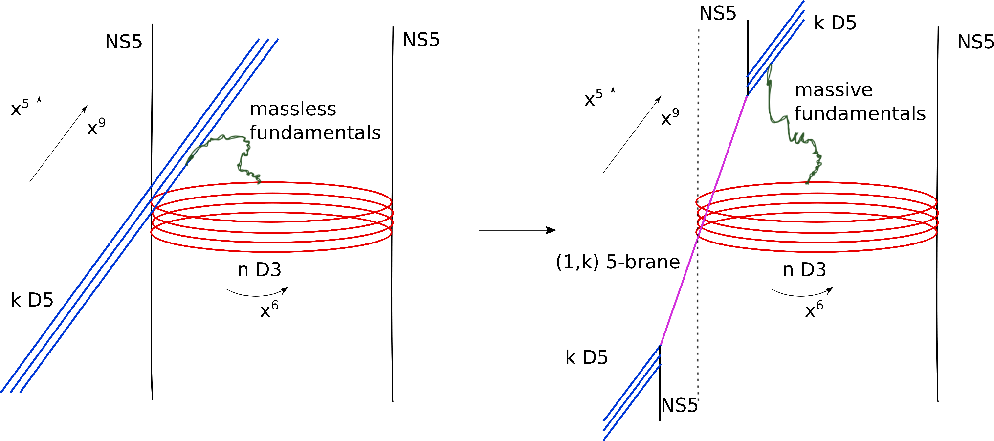
We have therefore managed to find a complicated brane configuration, the effective theory for which produces the desired Chern-Simons terms. The final step is to note that by rotating the five-brane relative to the NS5 sitting at by equal angles in the , and planes, the supersymmetry is enhanced from to [125, 126]. This completes the construction of our “base” IIB brane system, though we will return to it shortly to discuss how the supersymmetry gets enhanced beyond .
4.1.2 From branes to the ABJM geometry
The above brane construction can be related to M-theory and M2-branes through a series of duality transformations. We first map to type IIA string theory by T-dualising along . The D3-branes are now D2-branes along . At the same time the NS5-brane is mapped to a Kaluza-Klein monopole along , where is the compact direction T-dual to . On the other hand, the 5-brane gets mapped to a bound state of a Kaluza-Klein monopole along with units of D6-brane flux. Recall that this object lies along and also lies at a fixed angle in the planes.
The type IIA Kaluza-Klein monopoles that we have obtained are identical to the geometries which we reviewed around Eq. (1.7.12), the only difference being that now the circle that plays a crucial role in constructing the monopole is rather than the M-theory direction. We have seen that they correspond to purely gravitational solutions described by the metric [44, 98]
| (4.1.2) |
where , , and , with all the indices raised and lowered with the three-dimensional Euclidean metric.2828 28 There is a slight change in notation from Chapter 1. Here the vector field will be denoted rather than and we will use explicit index notation in place of vector notation (e.g. instead of ).
As previously explained in Chapter 1, this geometry describes a nontrivial circle fibration over ,2929 29 We will also use spherical coordinates for in what follows. where the circle shrinks to zero size at the origin. Moreover, requiring the absence of singularities imposes an “Dirac” quantisation condition on the flux of . A simple solution is when is a harmonic function with
| (4.1.3) |
where is a constant parametrising the size of the circle at infinity (we had earlier just set this to 1, but now it will become relevant), while . In the “near core” limit (), and via a coordinate change the geometry can be seen to reduce to a orbifold.
It is now time to reap the rewards of our efforts by lifting the whole configuration to M-theory. By going to strong coupling we decompactify the spatial direction and the D2-branes turn into M2-branes along . The Kaluza-Klein monopole associated with remains a Kaluza-Klein monopole in eleven dimensions. But recall that upon decompactification a pure D6-brane also turns into a Kaluza-Klein monopole associated with the M-theory circle, . As a result, the initial five-brane in our type IIB configuration, which becomes a Kaluza-Klein monopole carrying units of D6-brane flux after T-duality, now becomes a “tilted” Kaluza-Klein monopole in which the circle is a linear combination of and .
Therefore, the M-theory system constitutes exclusively of M2-branes extending in and probing a nontrivial 4-complex-dimensional background given by the superposition of the two Kaluza-Klein monopoles. This type of transverse geometry has been investigated in the literature and goes by the name of “toric hyper-Kähler,” in general preserving six bulk supercharges [127].
The metric, which we will shortly write down, is a generalisation of the Kaluza-Klein monopole that was written down in (4.1.2) above. In place of the single harmonic function , we will now require a positive-definite matrix of harmonic functions obeying
| (4.1.4) |
where and is the matrix inverse of . This condition can be shown to imply that each entry of is harmonic. Correspondingly there will be a matrix of vector fields that are related to via a generalisation of the usual relation between a vector field and a harmonic function,
| (4.1.5) |
This relation is required for the metric to be hyper-Kähler.
Because the Kaluza-Klein monopoles are tilted with respect to each other, the two sets of coordinates
| (4.1.6) |
play complementary roles in the metric. Moreover the metric has two angular coordinates and , with period , that label the two Kaluza-Klein circles in the problem and together parametrise a 2-torus. The modulus of this 2-torus is given by
| (4.1.7) |
With these preliminaries in place, the metric for the geometry under consideration can now be written as
| (4.1.8) |
Note that Eq. (4.1.5) implies the linear relation . Since the equations for and are linear, linear superpositions of simple solutions are also solutions to the supergravity equations, a feature that we will put to use below.
It is important to note that the modular parameter is acted upon by a set of fractional linear transformations which leave the torus invariant. Through Eq. (4.1.7) these induce a set of transformations on , where with . It turns out that a subgroup of the latter is a symmetry, generating new solutions of the eleven-dimensional supergravity equations [127]. In fact, a more general transformation of with is still a symmetry of the theory, although this now leads to a change in the asymptotic shape of the torus.
This knowledge can be put to work by allowing us to explicitly write down and study the geometry in which we are interested. The Kaluza-Klein monopole associated with the direction can easily be embedded in this eight-dimensional framework by choosing
| (4.1.9) |
It is a nice regular geometry (we have set of Eq. (4.1.3) to one). The other monopole, corresponding to what used to be the fivebrane in the IIB picture, is given by [98]
| (4.1.10) |
This is also a simple geometry. To see this, apply a transformation that acts as , while simultaneously taking and to keep the line element invariant, with
| (4.1.11) |
Under this, Eq. (4.1.10) is equivalent to
| (4.1.12) |
with new angles and modified periodicity respectively. The fact that and that the periodicity of the circles parametrising the torus has changed is a result of the transformation, which as we have mentioned above does not preserve the torus.
The final step is to combine (4.1.9) and (4.1.10) by linear superposition, such that the solution is given by , with . The nonzero elements of are then and the periodicity of the angles is as already discussed. In the limit where both and become simultaneously small (the regime where the two Kaluza-Klein monopoles “intersect” and we are near both cores) we can neglect the contribution from to obtain the “near-core” metric
| (4.1.13) |
Writing , and through the change of variables , we arrive at
| (4.1.14) |
Because of the identifications on the ’s, this looks like two copies of for a parametrisation in terms of spherical coordinates, where the orbifold acts on the three-sphere and is realised as the Hopf fibration .
Alternatively, we can make a final change of coordinates
| (4.1.15) |
to obtain
| (4.1.16) |
We see that the identifications can be simply expressed as and we have arrived at a orbifold of M-theory.
Thus, to summarise this section, our base system defined by a brane construction is dual to M2-branes transverse to a orbifold geometry. This orbifold has been studied previously in Refs. [128] and [129] and was discussed in the context of M2-branes in Ref. [119]. For general it is known to preserve supersymmetry in the bulk. This can be demonstrated using the following argument: The element of corresponding to the rotations is
| (4.1.17) |
and the preserved supersymmetries must be left invariant by the action of this group element. For generic this implies
| (4.1.18) |
One way to solve this is to take and another way is . In both cases there are 8 components of that survive. Naively this gives us preserved supersymmetries. However we have counted twice the supersymmetries that satisfy both conditions i.e. . There are 4 of these and thus we find independent supersymmetries. Note that these projectors imply and therefore placing M2-branes at the fixed-point of the orbifold does not break any more supersymmetry, as expected by the brane construction. Thus the corresponding worldvolume theory should have supersymmetry, which is what we have already found. Of course the cases are special. For there is no orbifold and for the orbifold is simply . Hence in these cases the background preserves and supersymmetries respectively.
4.1.3 From branes to the ABJM gauge theory
Having established the connection to M2-branes, let us now return to the gauge theory discussion. Even though at the end of Section 4.1.1 we recovered a theory with two Chern-Simons terms with equal but opposite levels, we still have the presence of Yang-Mills kinetic terms. This is addressed by taking the limit in which we decouple gravity from the brane worldvolume () and then looking at the theory for very low energies. Since in three-dimensions the standard Yang-Mills kinetic term is an IR-irrelevant operator,3030 30 Three-dimensional Yang-Mills is weakly coupled in the UV and strongly coupled in the IR. it drops out in this limit. One then arrives at a conformal Chern-Simons-matter gauge theory.
On general grounds the lagrangian of this theory must be captured by Eqs. (3.2.15)-(3.2.18) for some choice of structure constants . As we have already seen, it is possible to re-express the 3-algebra results of Section 3.2 in terms of a product Lie-algebra with bi-fundamental matter, by considering a triple-product . This re-expresses the twisted Chern-Simons term as a difference of two Chern-Simons terms with the same level and gauge group . Thus finally we have constructed the ABJM [98] theory
| (4.1.19) | |||||
where the sextic scalar potential is
| (4.1.20) |
The complex scalars and fermions transform in the bi-fundamental of the two gauge groups and also carry an R-symmetry index . The covariant derivatives act accordingly3131 31 Note that, in contrast to our notation in Chapter 3, we will work in “physics” conventions with hermitian generators when dealing with CS-matter actions in the Lie algebra formulation.
| (4.1.21) |
Finally, the piece
| (4.1.22) |
encodes the Chern-Simons terms for the gauge fields. Note that the Chern-Simons level plays the role of a (discrete) coupling constant in this theory.
We also collect the set of supersymmetry transformations that leave the above action invariant
| (4.1.23) | |||||
| (4.1.24) | |||||
| (4.1.25) | |||||
| (4.1.26) |
4.2 The ABJM proposal for AdS4/CFT3
We are finally in a position to see how the brane construction naturally leads to the formulation of an AdS/CFT duality [130, 131] as proposed by ABJM [98]. The superconformal CS-matter gauge theory with supersymmetry has a (discrete) gauge coupling . This theory is weakly coupled for large . For large , it also admits an ’t Hooft expansion in powers of . The planar diagrams have an effective ’t Hooft coupling , which can be kept small when . The claim is that, as in the correspondence between SYM and string theory on , the ABJM theory is dual to the geometry arising from the near-horizon limit of M2-branes on a orbifold singularity, which will turn out to be . The CS level is identified with the rank of the orbifold.
In order to see how this comes about, let us look at the near-horizon geometry of M2-branes on , which we derived in a previous section, in more detail. Let us start with , i.e. no orbifold. The near-horizon limit for the geometry generated by M2’s in gives rise to in the presence of units of 4-form flux [130, 131]. As originally pointed out in Ref. [132], it is convenient to think of as a Hopf fibration: a fibre bundle whose one-dimensional fibre is a circle, , and whose base is the 3-complex-dimensional manifold . This is denoted in the mathematics literature as . Reducing M-theory along the fibre, one recovers type IIA string theory compactified on . Notice that the fibration defines a specific direction within to be the M-direction along which we compactify.
Interestingly, even though the M-theory description is maximally supersymmetric, this is not what the IIA description sees. Following the recipe of Kaluza and Klein, zero modes cannot carry any momentum in the direction – in other words, they must be invariant under this U(1). Since the circle fibration is realised in a nontrivial manner, only some of the supercharges are invariant, and as a result the IIA theory ends up with or supersymmetry, depending on the orientation of the [132] (see also [133, 128]). Here we will choose the orientation, in order to match with the gauge theory result.
Now we can implement the orbifold action on the above construction. It reduces the factor in the near-horizon geometry to . This action commutes with, and therefore preserves, an subgroup of the isometry group of . The subgroup acts as a common phase on all the , while under the transform in the fundamental representation. As one would expect, is precisely the isometry group of for generic . In terms of the Hopf fibration, acts only on the fibre, reducing it to which is simply a circle times smaller in circumference than the original one. The factor of the isometry group acts as a shift along the fibre leaving the base unaffected, while the factor acts purely on the base.3232 32 The isometry group of is .
To summarise, the gravity dual to the Chern-Simons-matter theory at level is , with . This also suggests the existence of a parameter regime involving large , in which the gravity description should more appropriately be thought of in terms of IIA supergravity. Since the original spacetime preserved 16 supercharges, while the orbifold for generic preserves only 12, this is in line with usual AdS/CFT intuition which dictates that performing a quotient on the compact part of the geometry will lead to reduced supersymmetry. The supercharges preserved by the orbifold action are neutral under the and hence for the IIA and M-theory descriptions now both have the same amount of supersymmetry.
The metric of the near-horizon M-theory geometry has the form
| (4.2.1) |
with
| (4.2.2) |
where has period , is the radius of the sphere in Planck units, and we also have units of 4-form flux. The 1-form is related to the Kähler 2-form of by . The Fubini-Study metric and associated Kähler form are given in homogeneous coordinates by
| (4.2.3) | |||||
| (4.2.4) |
with .
The IIA geometry is closely related to the above via the usual reduction formulae. The string frame metric and dilaton are given in string units by
| (4.2.5) |
with units of four-form flux on and units of two-form flux on a .
Having established the geometry, let us see in which parameter regime each of the descriptions is valid. The most conservative statement of AdS/CFT would be that the planar sector of the large- ABJM theory should be dual to supergravity on . In principle, we expect the supergravity description to be good when the ’t Hooft coupling is large, , or . But when is the IIA description more appropriate than the M-theory one? For that one needs to have that the size of the circle in (4.2.1) be small, i.e. or . Hence, in the strong ’t Hooft coupling regime there are two supergravity descriptions of the theory depending on whether (IIA) or (11d SUGRA). This establishes all the theories involved in the conjecture and their respective regimes of validity.
The duality proposal has passed a great number of nontrivial of tests. For example, the spectrum of supergravity fields is in complete agreement with the spectrum of chiral primary operators from the gauge theory side [134]. This crucially requires the inclusion of monopole operators, which are to be discussed in detail in Section 6.1.1, after identifying the of the circle direction with of the gauge theory, (3.3.13). Moreover, at large the full superconformal index of the theory exactly agrees with the index over supersymmetric gravitons in [135, 136]. Details of the various tests and successes of the correspondence, as well as a discussions of properties like integrability, are beyond the scope of this work and the interested reader may wish to consult the reviews [137, 138, 139] and references therein.
In summary, the planar sector of the ABJM theory (valid for , when the theory is weakly coupled) is dual to type IIA supergravity on (valid for ) or eleven-dimensional supergravity on (valid for ).
It is worth remarking that the ABJM theory reproduces the expected scaling for the number of degrees of freedom for M2-branes: When the gauge theory is put on a thermal circle, the dual description is in terms of an AdS-black-hole geometry. The free energy of this black hole was estimated to scale as [140] and this is easily extended to the orbifold case, for which it has been argued in Ref. [98] that the scaling with is . This formula nicely reconciles the scaling at fixed (in particular ) that was predicted long ago in [140], and the scaling for the free energy of a large- gauge theory at fixed ’t Hooft coupling which requires that scale like .
These results are expected to be recovered by the statistical entropy of the massless modes on the worldvolume theory. Recent results on localisation [141] have allowed for this to be explicitly verified – albeit for the free energy of the Euclideanised ABJM model [142, 143] on (rather than ). This can be reduced to a matrix model that has a strong coupling expansion, the leading term of which beautifully reproduces both the scaling behaviour at fixed and the numerical coefficient of the gravity calculation [144]. For more details of this fascinating direction, the reader may consult Ref. [145]. Other multiple M2-brane and ABJM-related literature includes [146, 147, 148, 149, 150, 151, 152].
4.3 ABJ and discrete torsion
There exists a generalisation, due to Aharony, Bergman and Jafferis (ABJ) [153], of the ABJM model to the case where the matter fields are complex matrices in the bi-fundamental of . In this case and are and gauge fields. The form of the action is unchanged from the case.3333 33 Indeed, one can also consider the ABJM model with gauge groups. The coupling to bi-fundamental matter makes this a rather different theory with no generic spacetime interpretation. However, we will see in Section 5.3 that for these models are simply the theories and in some cases are dual to the M2-brane gauge theories. Let us assume without loss of generality that and write . Indeed, the action follows directly from the 3-algebra theory.
To understand these theories we return to the brane construction given above. We can easily generalise it to the case where the initial D3 segments involve different numbers of branes and , leading to Chern-Simons-matter theories which describe M-theory configurations with units of discrete torsion for the background 4-form. For this has the interpretation of M2-branes along with fractional M2’s stuck on the orbifold singularity. Starting from the same configuration one can also place an orientifold plane parallel to the D3’s, resulting in and theories corresponding to M2-branes on a singularity, where is the binary dihedral group of order [154, 155, 153].
Since the discrete torsion is only defined modulo , we see that for these models to match the supergravity we must make two conjectures:3434 34 Here the subscripts refer to the level of the corresponding Chern-Simons term in the lagrangian.
- 1.
has no supersymmetric vacuum if
and
- 1.
is dual to .
Note that both these conjectures are at strong coupling since cannot be made small for the models under consideration. We should also mention that in these models, the parity symmetry is typically broken as it maps .
5 Analysis of the theory I: basics
We have argued that the ABJM theory encodes the dynamics of multiple M2-branes probing a singularity. We proceed to find gauge-theoretic evidence for this by analysing the vacuum moduli space of the theory. We next look at the theory expanded around a particular point in the moduli space, obtained by allowing one of the scalars to develop a large vacuum expectation value. This will lead, via a novel Higgs mechanism, to the theory being recast in terms of three-dimensional super Yang-Mills after the scalar gets eaten by the Chern-Simons gauge field. At the end of this chapter we clarify the relationship between the ABJM and BLG theories.
5.1 Vacuum moduli space
The vacuum moduli space of a gauge theory is the space of vacua of the theory modulo gauge transformations. For D-branes in string theory, this is the space of vacua of supersymmetric Yang-Mills theory in the appropriate space-time dimension. Consider for example the theory on D3-branes, which is supersymmetric Yang-Mills theory in 3+1d with gauge group . This theory has six scalar fields , all in the adjoint representation. The classical potential is and is minimised by having all the scalars be diagonal matrices
| (5.1.1) |
Therefore the moduli space is naively , but we must remember that the Weyl group of permutes the eigenvalues. Quotienting by it, one finds the moduli space of D3-branes in flat space-time to be
| (5.1.2) |
This has a simple physical interpretation as the space of indistinguishable D3-branes, each one free to move in 6 transverse spatial dimensions. Because of the high degree of supersymmetry, this space does not receive quantum corrections.
One would like to understand the corresponding vacuum moduli space in the ABJM theory, which would provide a crucial test of the claim that it describes M2-branes. As we have seen, the structure of ABJM field theory is quite different from Yang-Mills, and moreover there is an additional ingredient: a orbifold. Therefore the moduli space needs to be computed and compared with that of indistinguishable M2-branes on the transverse space .
The vacuum moduli space was initially studied for BLG theory in [95, 118, 119] and these methods were then applied in [98] to study ABJM theory. We review these developments below, in this order.
5.1.1 Moduli space for BLG theory
We start by reviewing the results of Refs. [118, 119] on the moduli space of the theories. Subsequent to these works, it was realised [104] that there are actually two infinite families of such theories. Both have but one has gauge group while the other has gauge group . Here we wish to consider both, as they share the same lagrangian, so we present an updated version of the original analysis.
From the BLG sextic potential it is easy to see that the vacuum moduli space consists of 8 real scalars that are diagonal matrices. We combine them into four complex scalars and write them as
| (5.1.3) |
Gauge transformations take . There are two such transformations that keep diagonal. The first is a discrete transformation, which up to conjugacy may be taken to be . This identifies the configurations
| (5.1.4) |
and results in a quotient of the moduli space.
The second is a continuous gauge symmetry, with . For fields in the moduli space, the lagrangian reduces to
| (5.1.5) |
where gauges the symmetry, , and . Note the factor of in the Chern-Simons term that arises from taking the trace over matrices.
At this point we eliminate in favour of its field strength . We then treat as an independent field, subject to the Bianchi identity , which we impose via the Lagrange multiplier :
| (5.1.6) |
Integrating out leads to the identification . The Lagrange multiplier can now be absorbed in the by the redefinition
| (5.1.7) |
yielding the lagrangian
| (5.1.8) |
We will now show that the field is periodic. This arises from the fact that the fluxes of , the field strengths of , satisfy the Dirac quantisation condition. To see this, consider some field that couples to a field through . Let us now carry out parallel transport of over a closed path . The resulting field is related to the initial one by a transformation
| (5.1.9) |
Now using Stokes’ theorem we have where is a two-dimensional surface whose boundary is . Hence we may write
| (5.1.10) |
However the choice of is not unique. Given any two such choices and we require that the phase, viewed as an element of the gauge group , is the same. This implies that
| (5.1.11) |
and hence , where is any closed surface.
Applying this to the field , we have the quantisation condition
| (5.1.12) |
where the extra factor of 2 comes from the fact that is the sum of two independent field strengths. This holds in the case, while in the case the phase above must be equal to 1 only up to a action so the right hand side can be a half-integer or integer, which we denote by .
Converting the integral of over a surface into an integral of (in components, ) over the entire 3-volume,3535 35 For this manipulation it is best to temporarily continue to Euclidean 3-space. we find in the case that
| (5.1.13) |
whereas for we have
| (5.1.14) |
From the lagrangian Eq. (5.1.6) it follows that must have the periodicity for and for .
The result is the identification
which corresponds to a or quotient of the moduli space respectively.
The identifications from (5.1.4) and above do not commute; they generate the dihedral group3636 36 The dihedral group of order is given by . for or for . It follows that the moduli spaces of the two theories are:
| (5.1.18) |
In general, these moduli spaces do not have an obvious space-time interpretation in terms of M2-branes. However, we will see in Section 5.3.2 that such an interpretation can indeed be provided for the special values and 4.
5.1.2 Moduli space for ABJM theory
We now move on to consider the vacuum moduli space of ABJM theory. Here we must consider the minima of the potential Eq. (3.2.16). Because the potential is a perfect square, the scalars must satisfy . Contracting over and implies that and substituting back into shows that or
| (5.1.19) |
for all . Clearly this is solved if all the commute. Hence by a gauge transformation we can assume that
| (5.1.20) |
To see that this is the generic solution one can compute the mass matrix for the off-diagonal components and see that it is positive definite for generic vacua. However, as is familiar from D-brane theories, there are special points in the moduli space with enhanced gauge symmetry and extra massless states.
We must now quotient by the surviving gauge symmetries. In addition, unlike the case of D-branes, the vacuum is also invariant under continuous transformations generated by the Cartan subalgebra. These gauge transformations are trivial in the adjoint representation but not in the bi-fundamental representation. In particular, each couples to a gauge field obtained from the diagonal components of the gauge fields:
| (5.1.21) |
The lagrangian for the vacuum moduli becomes
| (5.1.22) |
where and (no sum on ). Note that the last term of the lagrangian above has an extra factor of compared to the analogous term in BLG theory.
Now, just as we did for that case, we introduce 2-forms and Lagrange multipliers which imply the Bianchi identities , from which locally can be written as for a set of 1-forms . Then the above lagrangian is equivalent to
| (5.1.23) |
In this lagrangian, the are independent fields. We can integrate them out, after performing an integration by parts in the last term, to find . Finally, can be eliminated by defining the fields whereupon the action becomes
| (5.1.24) |
Under the gauge transformation , we have . Thus are gauge invariant coordinates on the moduli space.
As before, the field satisfies the condition
| (5.1.25) |
where the integral is over 3-space. It follows that in the lagrangian Eq. (5.1.23), the contribution of the last term to the path integral is periodic under shifts of by for any integer , or in other words we must identify .
Returning to our gauge invariant variables we see that they are subject to the identification
| (5.1.26) |
Each parametrises not but rather the orbifold space . The collection of all the ’s then naively parametrises the product space . However at this point we again recall that we must quotient by the Weyl group, which is the symmetric group and permutes the copies in the product. As a result the moduli space of ABJM theory is
| (5.1.27) |
This has precisely the right form to be physically interpreted as the moduli space of indistinguishable M2-branes moving in a transverse space.
5.2 A novel Higgs mechanism
Let us re-examine the BLG theory, namely the , theory of Section 3.1. While we have not yet provided a definitive physical interpretation for it, it will be argued in Section 5.3.2 that for the special values it describes a pair of M2-branes in or . We now show [162] that upon giving a VEV to a scalar, it can be rewritten as maximally supersymmetric Yang-Mills theory in 2+1d with infinitely many corrections. In the process the pair of non-propagating Chern-Simons fields of BLG theory “eat up” a scalar and give rise to a single massless propagating vector field. Thus on the Coulomb branch, BLG theory has a propagating Yang-Mills field. This provides a key relation between its 3-algebra structure and the more familiar Lie algebra structure of Yang-Mills theories. The above considerations will then be extended to the ABJM case, where some new features arise. The novel Higgs mechanism provides a useful check of these theories and tests detailed features including the somewhat baroque Chern-Simons structure.
5.2.1 A simplified version
We first present a simple example of the novel Higgs mechanism that does not involve supersymmetry or 3-algebras. It is a property of a certain class of Chern-Simons theories in 2+1d, particularly those with difference-type actions.
Consider the Chern-Simons theory
| (5.2.1) |
where and . We would like to induce a particular type of mass matrix via the Higgs mechanism. Such a term arises by choosing a Higgs field in the bi-fundamental representation, for example the of , which transforms as
| (5.2.2) |
The covariant derivative on the Higgs field is then
| (5.2.3) |
For convenience we normalise the scalar kinetic term as
| (5.2.4) |
where this trace is, formally, unrelated to that in the gauge field action – here it just sums over two pairs of repeated indices in the fundamental representation, one pair being associated to each factor of . This kinetic term gives rise to the interaction:
| (5.2.5) |
With a Higgs VEV proportional to the identity, , the mass term is equal to
| (5.2.6) |
where now the trace is over the Lie algebra of after identifying the two factors in .
It is convenient to go to a different basis of gauge fields by taking the linear combinations
| (5.2.7) |
In these variables, and with the mass term, the lagrangian is
| (5.2.8) |
where is the standard non-abelian field strength for the vector field . From this follows the equation of motion for
| (5.2.9) |
We see that the field is algebraic. However, because of the quadratic term, it cannot be eliminated in a straightforward fashion. Instead one can solve the above equation recursively, to get:
| (5.2.10) |
The terms in the ellipsis above contain all powers of and the orders in this expansion are counted by the parameter .
We may now insert Eq. (5.2.10) back into the lagrangian of Eq. (5.2.8) to find:
| (5.2.11) |
In this process, a pair of non-propagating Chern-Simons gauge fields have been replaced by a single propagating, massless Yang-Mills type gauge field. Its single polarisation was gained by “eating" a component of the Higgs field. This is the novel Higgs mechanism [162]. The Yang-Mills coupling constant is .
Note, however, that there are still higher-order terms in . Taking allows us to ignore them, but then the Yang-Mills term becomes very strongly coupled. This can be avoided by simultaneously scaling keeping fixed [119]. In this latter limit the higher-order terms do drop out and the Yang-Mills coupling remains finite and can be chosen arbitrarily.
We now continue to describe the novel Higgs mechanism in BLG and ABJM theories where we will encounter both some subtleties – and a nice physical interpretation for the effect.
5.2.2 The Higgs mechanism for BLG theory
Recall that the BLG lagrangian is
| (5.2.12) |
where
The structure constants are given by the 4-index totally anti-symmetric symbol , with , and with the Chern-Simons coefficient quantised as , where . We also fix the Chern-Simons level to the value for the remainder of this section.
Consider the situation in which one of the transverse dimensions, say , develops a VEV. Because of invariance it is possible to rotate the scalar field that gets a VEV to have only the component . Thus the four indices split into plus , and this amounts to considering . Note that preserves supersymmetry as long as no other field has a VEV. To see this, consider the fermion supervariation (3.1.16). The first term on the RHS is zero because the scalar VEV is constant while the gauge field VEV is zero. The second term vanishes because can occur at most once and the other two scalar fields have vanishing VEV. Therefore the theory expanded about this scalar VEV has maximal supersymmetry.
Now let us examine the various terms in the lagrangian and show how they reproduce the desired SYM theory. To begin with, consider the sextic potential. Introduce the labels as well as . Then the potential is
| (5.2.13) |
In the last line we have inserted the VEV , which leads to a term quartic in the remaining ’s. Note that in this term, only appear where and . The terms of order and have not been written explicitly because they decouple in the limit , which we will eventually take.
Using where the latter is the 3-index totally anti-symmetric symbol and structure constant of an Lie algebra, we see that the quartic term becomes
| (5.2.14) |
which is precisely the quartic scalar interaction of maximally supersymmetric Yang-Mills theory in 2+1d.
Following the same procedure, it is easy to check that the 2-fermion, 2-scalar coupling reduces to the Yukawa coupling of 2+1d Yang-Mills, plus terms with two fermions and two scalars
| (5.2.15) |
We see that the only scalars and fermions appearing in the first term (which will be the leading term in the limit of large VEV) are and .
Since kinetic terms are unaffected by a scalar VEV, it only remains to understand the gauge field terms including couplings of gauge fields through covariant derivatives. On the face of it this should be the major stumbling block, for the gauge field in the 3-algebra theory only has Chern-Simons couplings while the D2-brane Yang-Mills theory requires a dynamical gauge field. As we are committed to make no additional assumptions to account for the dynamical gauge field, we simply work out the full content of the theory in the presence of the VEV of the scalar field . As before, we will see that the Higgs mechanism and the original Chern-Simons coupling conspire to provide the desired dynamical gauge field with all the right properties.
In view of our split of indices into and , it is natural to break up the gauge field into two parts
| (5.2.16) |
Each of these is a triplet of vector fields. We can now re-write the two terms in the Chern-Simons action as follows
| (5.2.17) |
We also need to consider the couplings arising from the covariant derivative on . We have
| (5.2.18) |
and
| (5.2.19) |
Inserting these in the lagrangian (but ignoring fermions) and using the VEV , we find the following terms involving
| (5.2.20) |
where we have defined a new covariant derivative which depends only on
| (5.2.21) |
Notice that the first term looks like a mass for , as might be expected from the Higgs mechanism, but we will see in a moment that is not in the spectrum of the theory.
The terms involving that come from the gauge field self-couplings are
| (5.2.22) |
where we have also defined
| (5.2.23) |
Thus is an auxiliary field appearing without derivatives. It can therefore be eliminated via its equation of motion. We can extract the leading part of such solution by temporarily neglecting the quadratic term in coming from the cubic self-interaction as well as terms coming from higher interactions with scalars. Later we will show that these would have led to higher-order contributions that are suppressed in the strong-coupling limit. We therefore consider the set of couplings
| (5.2.24) |
and find that
| (5.2.25) |
Thus one of our gauge fields, , has been set equal to the field strength of the other gauge field (plus other terms). Eliminating gives rise to a standard Yang-Mills kinetic term for ! This is the miracle that promotes the Chern-Simons gauge field into a dynamical gauge field.
Continuing with the computation, the sum of the Chern-Simons gauge field action and the scalar covariant kinetic terms becomes (up to a total derivative)
| (5.2.26) |
The redefinition
| (5.2.27) |
leads to
| (5.2.28) |
and
| (5.2.29) |
Thus Eq. (5.2.26) finally becomes
| (5.2.30) |
The terms in that we had neglected will lead to higher interactions with increasingly higher powers of in the numerator and in the denominator.
For the fermions, we easily find that
| (5.2.31) |
where on the LHS is the 3-algebra covariant derivative while on the right is the Yang-Mills covariant derivative.
The theory we have obtained now has an interacting Yang-Mills piece supplemented with some decoupled fields as well as a variety of higher-order terms.3737 37 The original 3-algebra still makes its presence in the higher-order terms, to be understood geometrically in the next section. The action can be written in the form
| (5.2.32) |
where
| (5.2.33) |
For the SU(2) part, we rescale the fields as , to find the action
| (5.2.34) |
where is the action of maximally supersymmetric 2+1d SU(2) Yang-Mills theory
| (5.2.35) |
with the field strength and covariant derivative defined as
| (5.2.36) |
In the above, are all completely independent of . Taking the limit , only the term remains. The interacting part of the surviving theory is precisely Yang-Mills, the low-energy theory on two D2-branes. Then, since scalar fields have canonical dimension , we can identify ; this is the correct mass dimension for the Yang-Mills coupling in 2+1d, and it is in agreement with the fact that this theory is weakly coupled in the UV and strongly coupled in the IR.
Note that has disappeared from the theory, while no longer has a Chern-Simons coupling but rather a full-fledged Yang-Mills kinetic term. The fields that survive in the D2-brane action have the correct couplings to the newly-dynamical gauge field. Note that the terms corresponding to the modes have disappeared; they played the role of the Goldstone bosons that gave a mass to , and at the end were transmuted via the Higgs mechanism and the Chern-Simons coupling into the single physical polarisation of .
One might be alarmed at the fact that the original gauge symmetry appears to have been Higgsed to by a VEV of a field in the of . That is not quite the case. The Higgs mechanism breaks to as it should, since the scalar that develops the VEV breaks to a diagonal . However, several free scalars are left over and the gauge field is obtained by dualising one of them.
The final theory also contains 8 non-interacting scalars . Of these, correspond to the centre-of-mass modes for the D2 worldvolume theory. The last scalar , the one which originally developed a VEV, can now be dualised via an abelian duality to yield an extra gauge field. The free abelian multiplet is completed by , so the full gauge group is SU(2) U(1). Note that the entire multiplet comes from a direction that was not central in the original 3-algebra (in the sense that it does not satisfy for all ).
When , the theory on the D2-branes becomes strongly coupled.3838 38 We remind the reader that at this stage we have fixed the Chern-Simons level, which is an otherwise free parameter of the theory, to . In the next section we will relax this assumption. As we have already seen, the physics of strongly coupled Yang-Mills in 2+1d is expected to be captured by M2-branes. Hence, in this limit of Yang-Mills one expects to recover the low-energy physics of 2 M2-branes in flat space [162].
While the novel Higgs mechanism plays a specific role in the context of M2-branes, as described above, it occurs quite generically in a class of Chern-Simons field theories in 2+1 dimensions. It is closely associated to the well-known phenomenon of topological mass generation in 2+1d and stems from a conflict between diagonalisability of kinetic and mass terms that arise in Chern-Simons type theories [163].
5.2.3 The Higgs mechanism for ABJM theory
We next turn our attention to applying the above mechanism to the case of the full ABJM theory [164, 165, 166]. Here, however, the bifundamental nature of the matter fields makes the technical discussion slightly different; it further involves a subtlety relating to the treatment of the abelian parts of the matter and gauge fields [167]. For the sake of simplicity, we focus our attention on the bosonic part of the action. In this case we will also reintroduce the -dependence. In fact, we will consider the Higgsing process in a limit where not only the VEV but also the Chern-Simons level is taken large, in such a way that .
Consider once again the ABJM lagrangian (4.1.19)
where
| (5.2.38) |
We would like to see what happens under a perturbation schematically of the form
| (5.2.39) |
with , or more precisely in terms of the real parts3939 39 Here the fields after Higgsing are hermitian matrices which will be expanded in a basis consisting of the unit matrix and a hermitian set of generators.
| (5.2.40) |
For the Higgsing it is appropriate to define
| (5.2.41) |
which, observing that , translates into
| (5.2.42) | |||||
| (5.2.43) | |||||
| (5.2.44) |
Note that the abelian gauge fields do not appear in the covariant derivative . In terms of these new variables the Chern-Simons part of the lagrangian becomes
| (5.2.45) |
The fields are matrices which can be expanded in terms of a complete basis of generators as follows4040 40 Here we normalise the generators as , with .
| (5.2.46) | |||||
| (5.2.47) | |||||
| (5.2.48) |
and subsequently, including the VEV and writing things in terms of real components,
| (5.2.49) |
As a result one gets for the covariant derivative
| (5.2.50) | |||||
where . Then we obtain
| (5.2.52) | |||||
Adding the following two terms, which are equal to zero by the Bianchi identity,
| (5.2.53) |
and with the inclusion of the Chern-Simons terms, we get that the action becomes
| (5.2.57) | |||||
where . The higher order terms also include a contribution proportional to . However, these terms are subleading in the limit and can be ignored.
At this point we can perform a shift in the and in the abelian component of the gauge field
| (5.2.58) |
which leads to
| (5.2.59) | |||||
where .
It is interesting to observe that in the above expression, both the and the components vanish to leading order. These fields make up the Goldstone modes that render, respectively, and dynamical to give back a gauge field. Without the vanishing of the one would have ended up with excessive degrees of freedom. We will see shortly that this also has an interpretation in terms of the M2’s moving in the orbifold geometry.
We can now integrate out both the abelian and non-abelian components of to obtain
| (5.2.60) |
and upon plugging into (5.2.59) this gives
| (5.2.61) |
Then using the definition
| (5.2.62) |
and taking the limit , with , the higher order terms drop out. Combining the remaining traceless part of with the trace part of , we find the bosonic kinetic terms for , three-dimensional Yang-Mills theory.
Regarding the bosonic potential terms, we observe that all terms scaling like vanish, so one is left with a potential that is of order , and hence fourth order in the scalar fields, as expected. The remaining terms are subleading in and vanish in the limit. The surviving term in this limit is
| (5.2.63) |
In this way we have recovered the full bosonic content of three-dimensional Yang-Mills by Higgsing the ABJM theory.
5.2.4 Higgsing and large- compactification
We now proceed to assign a spacetime interpretation to the field-theoretic mechanism that we have thus far described in the ABJM case. We have already established in Section 4.1.2 that the orbifold acts as on the complex coordinates transverse to the M2-brane worldvolume. Setting for simplicity reduces us to as , with4141 41 The trace parts of the field theory scalars are related to spacetime coordinates by multiplication with a factor of .
| (5.2.64) |
Expanding around with , we see that
| (5.2.65) |
should be an invariance of the theory, or by writing , that is compactified with radius . This is the radius of the M-theory circle. By letting , one recovers the theory of D2-branes of type IIA string theory in flat space.
In particular, since three-dimensional Yang-Mills involves seven (as opposed to eight) scalars, it is natural to expect that one of the Goldstone modes that render the gauge fields dynamical in the ABJM theory should be precisely , corresponding to the centre-of-mass motion of the branes in that direction. On the other hand, for the BLG model, the scalar degree of freedom that disappeared was exactly the one that developed the VEV. For our particular choice of VEV, this corresponds to being singled out, as opposed to , as implied by (5.2.65). This is a sign that the orbifold picture is not an appropriate dual description of the BLG model for generic values of . We will explicitly see in Section 5.3 that this is indeed the case.
The relation between the novel Higgs mechanism and large- compactification can also be understood as follows: can be thought of as a cone over . The orbifold action leads to an opening angle that shrinks like . In the limit where , this opening angle approaches zero, so at some point infinitely far out on the moduli space the local geometry approaches that of a cylinder , where the former is always realised as a Hopf fibration. However, then involves a base of infinite volume, while the fibre has a finite, tunable radius (which can be taken to be small) because of the action of the orbifold. Moreover, the nature of the fibration is locally trivial and the cylinder is really . The scaling limit , with , precisely takes the M2-branes out into this cylindrical space, where they should behave like D2-branes in type IIA string theory. So at low energies we expect a finitely coupled Yang-Mills theory – and that is exactly what we find [119, 167].
It is worth mentioning that the discussion in the limit of large-order orbifolds bears a strong resemblance to the ideas introduced in [168, 169] and used in the deconstruction approach to M5-branes [170, 171]. In those works the order of the orbifold grows large in a similar way and the D-branes are simultaneously moved far away from the fixed point, so that they effectively end up propagating on a cylinder. It is important to note that, compared to the starting quiver gauge theory, the deconstructed theory is higher dimensional and has enhanced supersymmetry. Another interesting point is the implementation of the Higgs mechanism for the ABJM model coupled to conformal supergravity, or “topologically gauged ABJM theory” [172]. The Higgsed theory [167] has broken conformal invariance and reduces to 3d “chiral supergravity” in the sense of [173]. The latter has an AdS3 vacuum and should also admit a CFT2 boundary description. Hence, the Higgs mechanism relates to in something that might be called “sequential AdS/CFT” [174, 175].
5.3 Relation of ABJM to BLG
At this stage we can close the circle of ideas by asking the following question: What is the relation of the original BLG theory of Section 3.1 to the ABJM models?
We first remind that for we can chose a basis for the 3-algebra of matrices given by
| (5.3.1) |
where and are the Hermitian Pauli matrices: . In this basis the structure constants and metric of the triple product defined in (3.3.1) are
| (5.3.2) |
Thus is real and totally anti-symmetric. In fact one can check that the , lagrangian constructed from this 3-algebra is the lagrangian with gauge symmetry but written in complex notation: , for . (See Section 3.3.1.)
Here we need to reiterate a subtlety that will be important for our discussion: The lagrangians are defined only in terms of the data of the Lie algebra and not the gauge group. This data is encoded by the 3-algebra. However to define the quantum theory we need to specify the gauge group and the choice of the latter has an effect through the flux quantisation conditions. Since more than one group can have the same Lie algebra we see that more than one theory can be associated to a lagrangian. To make this distinction clear in this section we refer to the lagrangian in terms of its Lie algebra, e.g. or , but we will refer to the theories in terms of their gauge group, e.g. , or .
We have seen in Section 3.3 that the models can be derived from the models by gauging the global . We now describe how to go backwards: namely integrating out the gauge field of the ABJM lagrangians leads to lagrangians, along with a orbifold action on the fields. In the case with we will show that the ABJM model can be related to the lagrangian with an additional orbifold. However there is global information that needs to be taken into account and this only works when and are relatively prime [104]. Let us next see how that happens.
5.3.1 From to CS-matter theories
To begin let us go back and rewrite the ABJM lagrangian as
| (5.3.3) |
As in Section 5.1.1, we introduce a Lagrange multiplier term
| (5.3.4) |
Integrating the last term by parts we find
| (5.3.5) |
We can now integrate out to see that
| (5.3.6) |
Thus under a gauge transformation one has that
| (5.3.7) |
Substituting back we find that the lagrangian is equivalent to the lagrangian with new variables:
| (5.3.8) |
The variables and are gauge invariant.
Most of the steps that we have outlined do not rely on the global choice for gauge group. The exception to this is the last step (5.3.8) where the infinitesimal gauge transformation was exponentiated to a finite group element. Thus we should be careful with some global issues. In particular, although the Lie-algebra decomposes as it is not true that . Rather one finds that is an -fold cover of . To see this, we note that the group homomorphism defined by covers -times. In fact, the determinant satisfies , but this only determines modulo . Thus we have , where is the centre of .
The upshot is that although (5.3.8) links the lagrangian of the theory to that of , the gauge group is and not .4242 42 One might have expected but only the relative factor acts non-trivially. As we will now see this leads to modified flux quantisation rules that affect the physical interpretation.
We next need to determine the periodicity of in (5.3.8), which follows from a quantisation condition on the flux . In this case the standard Dirac condition is modified. In particular, the gauge group is and we need only require that , i.e. the phases computed by two different paths and must be equal modulo . Thus we see that the quantisation condition is
| (5.3.9) |
As we have emphasised, this fractional flux quantisation condition arises because the gauge group is instead of , with the relative centre of the two factors. Thus we refer to the resulting Chern-Simons matter theory as the -theory. This is distinct from a theory with the same lagrangian but global gauge symmetry and no fractional flux quantisation, which we refer to as the -theory.
After integrating out , we are left with the condition . This is analogous to what we obtained for the moduli space calculation with the difference that now we are in the full theory, not just the moduli space. Locally, vanishes so that and must have the same flux. Note that we do not require that is globally defined so there can be a non-zero Wilson line for the gauge field . However, since in any open set where is single-valued, it follows that globally. This generalises the flux quantisation argument of [176] to allow for a non-vanishing but trivial gauge field and applies to the full theory, not just the moduli space (but only for the overall fluxes). Since we have
| (5.3.10) |
and has period . Note that since is a transformation, also has period . Thus we can fix the symmetry using (5.3.7) and set . However, this periodicity imposes an additional identification on the -invariant fields
| (5.3.11) |
We are therefore told that the ABJM theory is equivalent to a identification on the -theory. Note that the quotient arises here as the relative part of the two factors from .
However we need to be careful since there could be obstructions at a global level. To look for the latter it is insightful to compute the moduli space of the -theory along with a orbifold and compare it to the result.
For a general the vacuum moduli space is obtained by setting
| (5.3.12) |
If we consider gauge transformations of the form then behaves as if it were in the adjoint of and hence cannot tell the difference between the and theories. The result is that the gauge transformations which preserve the form of simply interchange the eigenvalues leading to the symmetric group acting on the M2-branes, just as is the case in D-brane theories.
Next we can consider transformations in the diagonal subgroup of or . These act to rotate the phases of the , however in the -theory they only do so up to the constraint that the diagonal elements must have unit determinant. In the -theory this is not the case and there are independent ’s, one for each , and each of these ’s leads to a identification on the moduli space. Thus for we indeed see that we find commuting copies of along with the symmetric group acting on the .
For the -theory, even including the action of , this will not always be the case. In particular, note that since the determinant of the gauge transformations coming from is always one we have, for an arbitrary element of the moduli space orbifold group,
| (5.3.13) |
Here represents a generic element of the moduli space orbifold group obtained in the -theory. On the other hand, the moduli space orbifold group of the -theory generated by independent ’s has
| (5.3.14) |
If these two theories are to give the same moduli space then we must be able to have for any possible combination of ’s. Thus we are required to solve
| (5.3.15) |
for as a function of , where is arbitrary. Hence, if this equation can be solved for then is an element of and can arise from the vacuum moduli space quotient group of the -theory.
We will now show that (5.3.15) has solutions for all if and only if and are co-prime. In general the solution is for any ; however we require that is an integer. It is clear that we may view and as elements of and we are therefore required to solve the following equation for
| (5.3.16) |
This always has solutions if the map is surjective on . Since is a finite set this will be the case if and only if is also injective. Thus we wish to show that implies . This is equivalent to showing that implies . Now suppose that . If and are co-prime then all the prime factors of must be in and all the prime factors of must be in . Thus . On the other hand if and have a common factor then we find a non-zero solution by taking and . Thus has no non-trivial solutions for if and only if and are co-prime.
This result can been restated as follows: Although locally , this is not true globally. Even though the lagrangian is defined by local information at the Lie-algebra level, the map we constructed, reducing the -theory to a quotient of the -theory, involves finite gauge transformations and is therefore sensitive to global properties of . The above discussion shows that the vacuum moduli space quotient group of the theories is not of the form , where , unless and are relatively prime [104].
We have therefore shown that if and have a common factor then the vacuum moduli spaces for the two theories do not agree, as there is a global obstruction to mapping the -theory to a quotient of the -theory. On the other hand, if and are co-prime then the vacuum moduli space calculated in the -theory, along with the identification coming from , agrees with the vacuum moduli space of the -theory. This suggest that there is no global obstruction and in these cases the theories are quotients of the theories. Thus one can conjecture that:
- 1.
is equivalent to a quotient of if and are relatively prime .
5.3.2 Connecting to the BLG models
We are finally in position to connect this discussion with the moduli space results for BLG theory, obtained in Section 5.1.1. Our analysis implies that for and odd, the ABJM models can be viewed as orbifolds of the model with gauge group . Clearly, for , the ABJM model for two M2-branes in is precisely the model of [83, 86, 85, 84].
One can also find a connection, which does not fit the above pattern, when the moduli space is . This arises from (5.1.18) for in the theory and for in the theory. It can be identified with the moduli spaces of two M2-branes in by introducing
| (5.3.17) |
so that in the language of Section 5.1.1,
| (5.3.18) | |||||
These are indeed the identifications expected for the moduli space of two M2-branes located at a orbifold singularity of M-theory.
Hence we have seen that for , the theory is precisely the ABJM model at level . We have also seen that the theory [118] and the theory [177] both have the correct moduli spaces to describe two M2-branes in . Indeed, there are two such theories expected, corresponding to the presence or absence of discrete torsion. Therefore it is natural to identify them with the ABJM and ABJ models respectively.
In summary, the following ABJ(M) theories are dual to BLG models:
- 1.
is dual to , both at ;
- 2.
is dual to , both at ;
- 3.
at is dual to at .
These proposed dualities have also been tested non-trivially by showing that their superconformal indices agree [177].
6 Analysis of the theory II: advanced topics
In this section we continue to analyse ABJM theory by investigating some of its most puzzling features. We start by focusing on the special role of momentum along the M-theory circle and its relation to “monopole” or “ ’t Hooft” operators. After this we discuss hidden symmetries arising at low values of the Chern-Simons level . We then include couplings to Ramond-Ramond background fields in the ABJM lagrangian and discuss the ensuing mass-deformed version of the theory. Finally, we discuss the physical and geometric interpretation for the vacua of the mass-deformed ABJM theory in terms of dielectric M2-branes in M-theory.
6.1 11D momentum, fluxes and ’t Hooft operators
Let us look more carefully at some subtle features of the ABJM lagrangian. For this we initially work with the theory and decompose the complex scalars into their magnitude and phase:4343 43 These ’s should not be confused with the coordinates introduced above Eq. (4.1.13). . Then the bosonic part of the lagrangian is
| (6.1.1) |
where as before we have defined and . Under a transformation we have and . Thus the centre-of-mass component can be set to zero by a gauge transformation. As we have already seen, this direction (the common phase of the four complex coordinates) plays the role of the M-theory circle. This leads to a puzzle: where has the eleven-dimensional momentum gone?
To answer this we compute the corresponding hamiltonian. The conjugate momenta are
| (6.1.2) | |||||
where . Thus the hamiltonian is
| (6.1.3) | |||||
where and .
We see that, as is always the case in gauge theories, the Hamilton equations for and impose constraints. In particular we have that
| (6.1.4) |
so that the magnetic fluxes of and are always equal. However, we also find
| (6.1.5) |
Thus we have established that turning on momentum around the M-theory circle is equivalent to turning on magnetic flux. Indeed, since and have quantised fluxes, we have and hence
so that
where is the total momentum. This is consistent with the orbifold which projects out momentum modes that are not a multiple of .
Let us now repeat this analysis for the general ABJM model. The lagrangian is
| (6.1.6) | |||||
where represent the Yukawa-type terms of the form . The hamiltonian is given by
| (6.1.7) | |||||
Thus we find the constraints
| (6.1.8) |
Let us look at the massless centre-of-mass modes. As was noted in the moduli space analysis of the previous chapter, in a generic vacuum the all commute. Thus we can write
| (6.1.9) |
and set the massive off-diagonal fields and fermions to zero. If we write , we find
| (6.1.10) |
which generalises the previous case to the centre-of-mass motion of each of the M2-branes. Thus we see once again that to include momentum modes around the M-theory circle we must turn on magnetic fluxes. In particular for the centre-of-mass coordinates we must turn on magnetic fluxes in the Cartan subalgebra, but more generally for any component of the fields we can introduce a corresponding flux to give it M-theory momentum [178, 98].
6.1.1 Group theory analysis of ’t Hooft operators
So far our discussion has been classical. However the relations (6.1.5) and (6.1.8) are constraints and as such we must also impose them in the quantum theory. Therefore we continue to identify flux quantisation with the momentum around the M-theory circle. However in the quantum theory we will need to include operators that create or destroy units of momentum and hence flux.
Such an operator is called an ’t Hooft operator (or sometimes a monopole operator). They were first introduced into gauge theories in [179] and can be specified by saying that they create a given flux through closed surfaces around some insertion point. So in other words the ’t Hooft operator is specified by giving the (Euclidean) spacetime point and flux – or equivalently, the singular behaviour of the gauge field at that point (in Euclidean space)
| (6.1.11) |
where is the magnetic flux, and is subject to the standard Dirac quantisation condition
| (6.1.12) |
These operators should be viewed as prescribing the behaviour of the fields at the insertion point in the path integral and hence are local.
A famous result of Goddard, Nuyts and Olive (GNO) [180] asserts that the solution to the Dirac quantisation condition is such that is determined, up to a gauge transformation, by a dominant weight of the ‘‘magnetic’’ dual gauge group.4444 44 We will have to assume some knowledge of group theory concepts at this stage, which can be found e.g. in [181]. This dual gauge group is more commonly referred to (especially in the mathematical literature) as the Langlands dual. Therefore, for a gauge group denoted by , the Langlands dual will be denoted by . The Dynkin diagram and hence the Lie algebra of the dual gauge group is obtained by mapping the simple roots of the original gauge group to the “co-roots”: . To obtain the actual dual group one notes that the weights obtained from the flux are in general a subset of all possible weights, corresponding to a dual group that is a quotient of the universal simply connected group associated to the dual Lie algebra. For example, as we will see shortly, the Langlands dual to is but the Langlands dual to is .
Let us illustrate this in the case at hand and for gauge group . By conjugation, which is simply the action of the gauge group, we can choose to have in the Cartan subalgebra
| (6.1.13) |
where generates the Cartan subalgebra of and 1l is the abelian generator (i.e. the identity operator). We can think of as a diagonal matrix in the fundamental representation with highest weight . The states in this representation are given by the orthogonal basis
| (6.1.14) |
where , are the simple roots of . In particular the diagonal components are4545 45 Note that we are using to indicate the range as well as to avoid introducing additional symbols.
| (6.1.15) |
and the quantisation condition is simply that , .
Following GNO, should be a weight of so we start by writing . The , are called the “fundamental” weights of and are by definition dual to the roots : .4646 46 The that we used in (6.1.14) are the fundamental weights of and dual to the co-roots. Fundamental weights form a basis in which we can expand any weight of the group. To determine the coefficients in terms of the fluxes we note that, for , we have . On the other hand we see that, from the basis (6.1.14) and definition (6.1.15),
| (6.1.16) |
Thus we find
| (6.1.17) |
which is indeed a weight of since the ’s are quantised. We also need to specify the abelian charge . To fix this we see that by tracing over Eq. (6.1.13) we get and therefore
| (6.1.18) |
The observation of GNO is that within the Cartan subalgebra we can still act with gauge symmetries (which are just conjugations) in the Weyl subgroup to order the diagonal components, . In this case is what is called a “dominant” weight of . An important result in representation theory states that dominant weights are in one-to-one correspondence with finite dimensional irreducible representations of the group. Hence, appropriate choices of fluxes fully characterise irreducible representations of , with the coefficients of (6.1.17) playing the role of Dynkin labels.
In fact, for we have no restrictions on and one can clearly arrange for any weight by choosing the appropriately. Moreover, for this particular choice of group and in our normalisations, and thus the Langlands dual to is .
However, it is interesting to note that all weights need not always arise: Consider , where we must impose the constraint . In this case one can show that can also be written as
| (6.1.19) |
and is therefore also a root of .4747 47 One can recover the expansion (6.1.17) from (6.1.19) by simply using the root inner products. These can in turn be read off from the Cartan matrix of . Roots are weights of the adjoint representation, which in turn is blind to the centre of the group. This means that the only representations that appear are those of and the Langlands dual to is .
Since dominant weights arise as the highest weights of finite dimensional irreducible representations, GNO also conjectured that monopoles come in representations of the dual group with highest weight . To see how this works in a familiar physical example, consider 4-dimensional maximally supersymmetric gauge theory. The perturbative spectrum contains gauge fields in the adjoint representation. The nonperturbative spectrum includes monopoles corresponding to a given flux. In particular the monopole and anti-monopole have , but are both mapped by the GNO prescription to the single highest weight . Nevertheless these monopoles are physically distinct, despite the fact that their fluxes can be mapped to each other by a gauge transformation, because the theory is also specified by the VEV of the scalar fields. In other words, the monopole is determined by a scalar field of the form
| (6.1.20) |
and thus the gauge transformation that maps also changes the vacuum. If we ask that we keep the vacuum fixed then we can no longer use gauge transformations to map into the form with . In this case one sees that the monopole and anti-monopole, along with the zero-flux state, form a representation of with highest weight corresponding to the adjoint representation.
Another example is the case of with highest weight and charge , corresponding to the symmetric representation. The fluxes in this representation are easily found to be
| (6.1.21) |
Although some of the fluxes can be mapped to each other using gauge transformations, they correspond to physically distinct monopoles in the gauge theory. Such gauge transformations also act on the VEVs of the scalar fields, so they cannot be used to identify fluxes. Therefore in a generic vacuum, the fluxes within a representation are physically distinct. This implies that the ’t Hooft operators assemble into multiplets that transform under the dual gauge group. In the next section we will see that in a Chern-Simons gauge theory, the ’t Hooft operators transform in representations of the dual gauge group that are indeed determined by the fluxes.
We also note that the second flux in this representation:
| (6.1.22) |
is already ordered to and thus maps to the dominant weight . One may try to view this as the highest weight of the anti-fundamental representation of . However since it has charge this cannot be viewed as a representation of (but rather ).
6.1.2 ’t Hooft operators in ABJM
Let us now consider ’t Hooft operators in Chern-Simons theories and in particular ABJM. More detailed discussions can be found in [182, 183, 184, 134, 185, 186, 187, 188, 189, 190, 191, 192, 193]. In particular, let us take the Euclideanised theory and denote by an ’t Hooft operator which creates a flux
| (6.1.23) |
on arbitrarily small spheres surrounding the point . An alternative view of ’t Hooft operators can be found in conformal field theory using the operator-state mapping. In particular, through conformally mapping to one can replace the insertion of an ’t Hooft operator at a point to the creation of a state at which carries magnetic flux through .
Our first observation is that, because of the Chern-Simons term, a single ’t Hooft operator is not invariant under gauge transformations. Since the flux lies in the Cartan subalgebra, the ’t Hooft operator breaks the gauge group down to the diagonal subgroup. To see how the ’t Hooft operator transforms under this group, consider an infinitesimal gauge transformation generated by , which we assume to vanish at infinity. Although the flux remains unchanged, because of the Chern-Simons term we find
| (6.1.24) | |||||
Thus an ’t Hooft operator that creates a given flux is not gauge invariant. However, by taking several such ’t Hooft operators together, we can create a multiplet of local operators that transforms under some representation of the gauge group. To obtain the transformation of under the full gauge group, we use the method of induced representations, based on the charges of ’t Hooft operators under the subgroup. Hence we see that, following the GNO map from charges to weights constructed above, we can identify a multiplet of ’t Hooft operators with the various operators obtained from fluxes that appear in an irreducible representation with highest weight
| (6.1.25) |
In particular, the charges of the states in this representation agree with (6.1.24), essentially by construction. We note that the second factor is not a dominant weight but rather the negative of a dominant weight. We therefore identify the representation of the factor as the Cartan dual representation of (whose lowest weight is ) and in order to avoid unnecessary notation we will not always write out the two factors of the highest weight. Thus taking the multiplet of operators corresponding to the fluxes found in the representation with highest weight we obtain an ’t Hooft operator
| (6.1.26) |
which transforms under gauge transformations in the representation of with highest weight .
Secondly, we want to consider supersymmetric ’t Hooft operators. This means that the classical field configuration near the insertion point needs to preserve some fraction of the supersymmetry. As we will see, this means that in addition to a singularity in the gauge field, we must also require a singularity in the scalar fields. Assuming that the fermions vanish and that the scalar fields remain in the vacuum moduli space - i.e. commuting but not necessarily constant - the supersymmetry variation is
To proceed we note that we are looking in the Euclidean regime. In such cases we do not need to look for real solutions. In particular if we expand in terms of real scalars then when we look for solutions in the Euclidean regime we no longer require that , be real. This means that we should not identify and as complex conjugates of each other but rather as independent fields. Similarly we no longer require that , although we still impose [185].
With this in mind we can find supersymmetric configurations by taking a single scalar, say , and setting
but not . This will then preserve the supersymmetries , i.e. half. Note that since we do not assume that the remaining supersymmetries , and are not related to and hence can still be non-vanishing.
The equations of motion for the gauge field can now be written as
| (6.1.27) | |||||
Note that if remains in the vacuum moduli space, i.e. commuting, then . In addition the Bianchi identity implies that . Thus a supersymmetric ’t Hooft operator is determined by an harmonic function which takes values in the Cartan-subalgebra and whose pole defines the magnetic charge , c.f. (6.1.11):
| (6.1.28) |
The ’t Hooft operators can be used to construct important observables in ABJM. As we have seen they are crucial for obtaining states with momentum around the M-theory circle. Indeed the circle action corresponds to rotations which have been gauged. Thus if we try to construct gauge invariant operators out of the local fields then they must be neutral with respect to and hence have zero momentum around the M-theory circle. For example if we concentrate on the scalars then the only gauge invariant operators are analogues of spin-chains in the AdS5/CFT4 correspondence:
| (6.1.29) |
But these all carry zero charge and hence are invariant under rotations of the M-theory circle. However, we can rectify this by allowing operators such as
| (6.1.30) |
so long as is an ’t Hooft operator with charge and is in the dual to the symmetric representation of . This corresponds to highest weight vector
| (6.1.31) |
and hence to , . Note once again that this exists as long as is a multiple of , i.e. it only allows for eleven-dimensional momenta that are multiples of , in agreement with expectations from the orbifold projection.
6.1.3 Abelian ’t Hooft operators
The ’t Hooft operators that we have discussed might seem somewhat abstract in nature. So let us try to shed some light on these operators in the simpler abelian case. In fact, we have already seen examples of abelian ’t Hooft operators – the exponentials – in the moduli space computation of Section 5.1. Imagine now that we are working with ABJM theory.
Let us first write down the total charges under the groups and obtained by taking the difference and sum, respectively, of the gauge fields in the original groups
| (6.1.32) |
Both of the total charges are constrained to be zero by gauge invariance. The second equation says the fluxes associated to are equal while the first equation equates the common flux to the charge coming from the matter current (which in turn we have identified with momentum in the M-direction).
Now recall from the analysis following Eq. (5.1.23) that the fields obtained by dualising are shifted by under the subgroup. It follows that
| (6.1.33) |
has charge under this subgroup. Furthermore inserting factors of into the path integral
| (6.1.34) |
with given by (5.1.23), is equivalent to shifting
| (6.1.35) |
i.e. it has created units of flux in the and subgroups with the singularity located at . The gauge invariant coordinate on the moduli space is then identified with .
In this simple abelian case we also see that the ’t Hooft operator is just a Wilson line for the gauge field
| (6.1.36) |
where we used the fact, derived after Eq. (5.1.23), that . The integral is over a curve that ends at the spacetime point with some some starting fixed reference point (that we could take to be at infinity). However such an interpretation is not possible in the non-abelian theory and one must use the definition above in terms of singularities of the fields in the path integral.
In the abelian example we can also see some important quantum properties of ’t Hooft operators that we expect to also be valid in the non-abelian case. One such property is that the ’t Hooft operator is covariantly constant
| (6.1.37) |
This is more generally true for any , an operator that has charge , since the covariant derivative changes accordingly. Because of the absence of singularities (see below) this can be thought of as the product of coincident ’t Hooft operators.
A related point is that, in conformal field theory, has dimension zero. This is clear classically since should have dimension one, but one may wonder whether or not it holds in the quantum theory. After all, in perturbative string theory we are used to the notion that, due to normal ordering effects, the free boson vertex operator is not dimensionless but rather has conformal dimension . However in the present case, since the momentum conjugate to is , there is no normal ordering ambiguity in the definition of , and therefore it has dimension zero also in the quantum theory.
In fact this argument strongly suggests that ’t Hooft operators have dimension zero in the full ABJM theory. To see this first consider a vacuum where the scalar field VEV’s have been sent to infinity. Here the theory is purely abelian and as above the ’t Hooft operators have dimension zero. Let us now allow for finite scalar VEV’s. Since the scalar VEV’s have conformal-dimension in three-dimensions, the conformal dimension of ’t Hooft operators cannot depend on them. Hence the ’t Hooft operators remain dimension zero at finite values of the scalar VEV’s in the full ABJM theory. For alternative and more detailed discussions on the dimensions and R-charges of ’t Hooft operators in Chern-Simons gauge theories, see [186].
It is important to remember that although ’t Hooft operators have dimension zero, they can still have non-trivial OPE’s with other local operators. In the abelian case one finds that does not commute with , leading to a non-vanishing OPE representing the creation of magnetic charge at the insertion point of . In the non-abelian case we should expect ’t Hooft operators that are, roughly speaking, constructed from , to have non-trivial OPEs with local operators constructed from . Since such ’t Hooft operators are not the identity, these Chern-Simons models describe logarithmic conformal field theories and hence are not unitary. This is due to the indefinite metric associated to the gauge fields which, although non-unitary in a formal sense, still leads to a unitary physical theory.
6.2 Hidden symmetries at
The derivation of the ABJM model applies even when . However, in that case the M2-branes are propagating in or so their worldvolume theory should preserve supersymmetry. This is not manifest in the lagrangian formulation. On the other hand, the brane derivation of the ABJM model implies that the full supersymmetry must somehow be present. The first step towards resolving this issue is to note that for the theory is strongly coupled. Therefore the quantum theory can in principle have quite different properties to the classical theory, including additional symmetries.4848 48 This is rather like the opposite of an anomaly, in the sense that the classical lagrangian does not have all the symmetries of the quantum theory. Consequently, one can propose that the additional supersymmetries, even if not manifest in the lagrangian, are present in the quantum theory.
We start with the observation that the two extra supercurrents are charged under . Naively, there are no gauge invariant local observables that can carry such a charge. Therefore, to make them gauge invariant, we must introduce ’t Hooft operators. Let us see how this works in the special case of .
First note that the ABJM model should have an R-symmetry. There is a manifest symmetry which at the quantum level is generated by the currents
| (6.2.1) |
To enhance this to we need currents of the form but these are not gauge invariant. However, we can rectify this by including ’t Hooft operators with charge and which are in the symmetric representation (so that )
| (6.2.2) |
where is the highest weight of the symmetric (anti-fundamental) representation. This is obtained by taking the flux , and only exists precisely when .
In addition there should be an extra supersymmetry current at . In this case we can construct
| (6.2.3) |
which has all the desired properties.4949 49 For related treatments see [187, 188, 194].
Finally at there should be a current that generates translations along the M-theory circle. A natural candidate for this is
| (6.2.4) |
where is the highest weight of the anti-fundamental with charge and can only arise at with , .
Thus we see that there are candidate operators that can enhance supersymmetry and translational invariance exactly as expected on physical grounds when . These operators necessarily involve ’t Hooft operators in an important way. It is a different matter to rigorously prove that the operators constructed above actually achieve the desired result, a task we will not attempt here.
6.3 Background fields
For a single M2-brane propagating in an eleven-dimensional spacetime with coordinates , the full non-linear effective action including fermions and -symmetry was discussed in Section 1.4. The bosonic part of the effective action is [9]
| (6.3.1) | |||||
So far the topic of this review has been on the non-abelian generalisation of the first term, in the decoupling limit while keeping finite, corresponding to multiple M2-branes propagating in flat space (or orbifolds of flat space). We now switch gears and focus on the generalisation of the second term, namely the coupling of multiple M2-branes to the background M-theory gauge fields.
In the well studied case of D-branes, where the low energy effective theory is a maximally supersymmetric Yang-Mills gauge theory with fields in the adjoint representation, the appropriate generalisation was given by Myers [195]. In the case of multiple M2-branes, the scalar fields and fermions now take values in a 3-algebra which carries a bi-fundamental representation of the gauge group. Here we will follow closely reference [196] and we refer the reader there for more technical details. In addition we will restrict ourselves to terms which survive under . For alternative discussions of the coupling of multiple M2-branes to background fields, including terms that do not survive this limit, see [197, 198, 199, 200].
6.3.1 BLG theory
Let us first consider the maximally supersymmetric case. Assuming that there is no metric dependence we start with the most general form for a non-abelian pull-back of the background gauge fields to the M2-brane worldvolume
| (6.3.2) | |||||
where are dimensionless constants that we have included for generality. The ellipsis denotes terms that are proportional to negative powers of and hence vanish in the limit .
Let us make several comments. First note that we have allowed the possibility of higher powers of the background fields. In D-branes the Myers terms are linear in the Ramond-Ramond fields, but they also include non-linear couplings to the NS-NS 2-form. Since all these fields come from the M-theory 3-form or 6-form, this suggests that we allow for a non-linear dependence in the M2-brane action.
Also note that gauge invariance rules out any terms where the -fields have an odd number of indices that are transverse to the M2-branes. For this is expected from the spacetime interpretation, where the theory with gauge group or , respectively, describes M2-branes on a orbifold, as discussed in Section 5.3.2. For these cases we must set to zero any components of or with an odd number of indices. Therefore, in what follows, we will restrict our attention to the case with . (Similar results hold for . However, in that case, ’t Hooft operators play an important role in restoring translational invariance.)
The first term in Eq. (6.3.2) is the ordinary coupling of an M2-brane to the background 3-form. Hence we should take for M2’s. The second term leads to a non-Lorentz invariant modification of the effective three-dimensional kinetic energy. It is also present in the case of a single M2-brane action (6.3.1), where we find . We will assume the same to be true in the non-abelian theory. The final term, proportional to , in fact vanishes because which is symmetric under . Note that we have allowed the M2-brane to couple to both the 3-form gauge field and its electromagnetic 6-form dual, defined by , where is defined in (1.5.2).
The equations of motion of eleven-dimensional supergravity imply that . However is not gauge invariant under . Thus is not obviously gauge invariant or even local as a functional of the eleven-dimensional gauge fields. We would like to find an expression that is manifestly gauge invariant.
To discuss the gauge invariance under , we first integrate by parts and discard all boundary terms. We find
| (6.3.3) | |||||
where we have used the fact that and have been projected out by the orbifold and hence and . We see that contains a coupling to the worldvolume gauge field strength , but this term is not invariant under the gauge transformation . However, it can be cancelled by adding the term
| (6.3.4) |
to . Such terms involving the worldvolume gauge field strength also arise in the action of multiple D-branes.
Next consider the terms on the third line of Eq. (6.3.3). Although is not gauge invariant, the combination is. Thus we also add the term
| (6.3.5) |
and obtain a gauge invariant action.
To summarise, we find that the total flux terms are, in the limit ,
| (6.3.6) | |||||
We will argue later that by comparing the higher order terms in fluxes that are demanded by supersymmetry with those obtained because the supergravity background is no longer flat at quadratic order.
Now let us supersymmetrise (6.3.6) in a fixed (but gauge-invariant) background.5050 50 Similar calculations appear in [201, 202, 203] where the flux-induced fermion masses on D-branes were obtained. Thus we consider a background in which
| (6.3.7) |
where
| (6.3.8) | |||||
and is assumed to be constant. After supersymmetrisation, one finds the lagrangian to be
| (6.3.9) |
where is the lagrangian (3.1.22) and
| (6.3.10) |
with
| (6.3.11) |
and .
Next we need to modify the supersymmetry transformations to accommodate the flux terms. One finds that the required choice is
| (6.3.12) | ||||
Invariance follows if is self-dual and
| (6.3.13) |
The superalgebra can be shown to close on-shell.
6.3.2 ABJM theory
Let us now consider the more general case of supersymmetry and in particular the ABJM [98] and ABJ [153] models. Following the discussion of the previous section, we start with
| (6.3.15) | |||||
Integrating by parts we again find a non-gauge invariant term proportional to which is canceled by adding
| (6.3.16) |
As was the case with the theory, we must also add
| (6.3.17) |
to ensure that the last term is gauge invariant. Thus in total we have
| (6.3.18) | |||||
Continuing as before, we wish to supersymmetrise the action
| (6.3.19) |
where is the Chern-Simons-matter lagrangian Eq. (4.1.19). We restrict to backgrounds where
| (6.3.20) |
with
| (6.3.21) | |||||
We can supersymmetrise this term if we take to be
| (6.3.22) |
and include the following modification to the fermion supersymmetry variation
| (6.3.23) |
We then find that supersymmetry requires
| (6.3.24) |
It also restricts to have the form
| (6.3.25) |
with . As a consequence, we find that
| (6.3.26) |
where .
6.3.3 Background curvature
It is interesting to understand the physical origin of the mass-squared term in the effective action Eq. (6.3.22), which is quadratic in the flux. Note that this term is a simple, -invariant mass term for all the scalar fields. Furthermore it does not depend on any non-abelian features of the theory. Therefore we can derive this term by simply considering a single M2-brane and compute the unknown constant .
We can understand the origin of this term as follows. We have just seen that it arises as a consequence of supersymmetry. For a single M2-brane, supersymmetry arises as a consequence of -symmetry and -symmetry is valid whenever an M2-brane is propagating in a background that satisfies the equations of motion of eleven-dimensional supergravity [9].
The multiple M2-brane actions implicitly assume that the background is simply flat space or an orbifold thereof. However, the inclusion of non-trivial flux implies that there is now a source for the eleven-dimensional metric, which is of order flux-squared. Thus for there to be -symmetry and hence supersymmetry it follows that the background must be curved. This in turn will lead to a potential in the effective action of an M2-brane. In particular given a 4-form flux , the bosonic equations of eleven-dimensional supergravity are
| (6.3.28) |
At lowest order in the fluxes we see that and is constant. However at second order there are source terms. To start, we assume that, at lowest order, only is non-vanishing. To solve these equations we introduce a non-trivial metric of the form
| (6.3.29) |
where and .
Let us look at an M2-brane in this background. The first term in the action (6.3.1) is
| (6.3.30) | |||||
Next we note that, in the decoupling limit , we can expand
| (6.3.31) |
and
| (6.3.32) |
so that
| (6.3.33) |
where the ellipsis denotes terms that vanish as . Thus we see that in the decoupling limit we obtain the mass term for the scalars. Similar mass terms for M2-branes were also studied in [208] for pp-waves.
To compute the warp-factor we can expand , where is second order in the fluxes, and linearise the Einstein equation. If we impose the gauge , then Einstein’s equations reduce to
| (6.3.34) |
and hence, to leading order in the fluxes,
| (6.3.35) |
Thus contributes the term
| (6.3.36) |
to the potential.
Next we must look at the second term, the Wess-Zumino term, in (6.3.1)
| (6.3.37) |
Although we have assumed that at leading order, the -field equation of motion implies that is second order in . In particular if we write we find, assuming is self-dual, the equation
| (6.3.38) |
The solution is
| (6.3.39) |
Thus we find that gives a second contribution to the scalar potential
| (6.3.40) |
Note that this is equal to the scalar potential derived from in Eq. (6.3.36). Therefore if we were to break supersymmetry and consider anti-M2-branes, where the sign of the Wess-Zumino term changes, we would not find a mass for the scalars.
6.4 Dielectric membranes
Having obtained the explicit form of the supersymmetric lagrangian for the mass-deformed ABJM model, Eq. (6.3.19), we can proceed to study the physics it describes. We recall that the undeformed ABJM action is given by the expression
where on the first line we have the Chern-Simons gauge field and the matter kinetic terms, while on the second we have the sextic scalar potential. Focusing on the purely bosonic sector will prove enough for our purposes.
By splitting , where , the mass deformation (6.3.27) changes the potential to
| (6.4.2) |
where
| (6.4.3) |
which in principle also involves a mass term for the fermions. Note that the expressions in (6.4.3) couple with and break the invariance. Nevertheless, in the full scalar potential (6.4.2), the terms that couple and cancel out [207]. As a result, we will keep a different notation for their respective indices, with and for . We conclude that the R-symmetry is broken down to the subgroup .
6.4.1 Vacua of the mass-deformed theory
From the previous sections we see that the supersymmetric vacua of the mass-deformed theory satisfy
| (6.4.4) |
where has the form
| (6.4.5) |
For maximally supersymmetric vacua we require that this is true for all
| (6.4.6) |
Taking the trace over implies that
| (6.4.7) |
Substituting back we find that Eq. (6.4.6) is only satisfied if or .
Thus the mass-deformed theory has two sets of ground states expressed in terms of the scalars and . One set corresponds to having and satisfying
| (6.4.8) |
as can be easily seen from (6.4.2)-(6.4.3). This can be solved by the ansatz
| (6.4.9) |
where and the ’s are a set of complex, constant, bi-fundamental matrices satisfying
| (6.4.10) |
There exist irreducible solutions to the above equation, explicitly given by [207]
| (6.4.11) | |||
| (6.4.12) | |||
| (6.4.13) | |||
| (6.4.14) |
Another set has , , with the ’s satisfying once again (6.4.10). Moreover, one can easily construct reducible solutions using the above irreducible representations to form block diagonal matrices with block sizes that add up to . It is also possible to construct reducible solutions where both and are turned on, as long as the block components of are zero when the respective ones of are not, and vice-versa so that (6.4.10) is satisfied for each block [207].
What is the expected physical interpretation of these vacua in the context of M2-branes? By taking into consideration the background geometry that gives rise to the mass-deformed theory in the previous section, one would anticipate that we have described an M-theoretic version of the “dielectric” Myers effect [195]. That is, in the presence of the 4-form flux, the M2-branes are supposed to puff up into a fuzzy (or non-commutative) 3-sphere in the transverse 8-dimensional space, with the non-commutativity scale set by . In the large- limit, the resulting configuration is an M2-M5 bound state and should also admit an equivalent interpretation in terms of a single M5-brane wrapping the [209]. In the following we will confirm this expectation.
6.4.2 Geometric interpretation and Hopf fibration
Let us examine how this picture emerges from the matrices (6.4.11) for our initial configurations with , . At closer inspection, as seen from (6.4.11), and one has three real degrees of freedom, as opposed to the four needed for the description of the expected 3-sphere. Moreover, the R-symmetry of the mass-deformed theory is only so the 3-sphere cannot be realised in the familiar -invariant way.
The key observation is that the following matrix combinations [62]
| (6.4.15) |
are adjoint matrices and symmetry generators. One can extract the parts as follows
| (6.4.16) | |||||
| (6.4.17) |
where are the transpose of the Pauli matrices. The and ’s then satisfy the commutation relations
| (6.4.18) |
Using these relations along with (6.4.10), one finds that the , as well as all bi-fundamental fields, transform under the combined action
| (6.4.19) |
and as a result only a single diagonal survives as a symmetry of the system.
In order to further analyse the geometry, one can use the well established fact that the algebra of large matrices, transforming in irreducible representations of a given symmetry group, approximates the algebra of functions on spaces with the same isometries. Or conversely, the matrix algebras can provide a finite-dimensional truncation/discretisation/quantisation of the continuous, “classical” geometry. Hence, one can define to leading order in the large- limit
| (6.4.20) |
which play the role of standard Euclidean coordinates on two, at-first-sight-different, ’s.
One can similarly define
| (6.4.21) |
as some yet-to-be-understood commuting classical objects. In terms of the above definitions, the relations (6.4.16) become
| (6.4.22) | |||||
| (6.4.23) |
i.e. in this limit and one has two versions of the same Euclidean coordinate on a single sphere. This is in line with our previous observation, stating that the solution has only one symmetry.
How does all this information fit together? The answer lies in recognising that (6.4.22) is nothing but the expression for the familiar first Hopf map from the unit 3-sphere to the unit 2-sphere. Note that in the above construction the 2-sphere coordinates are invariant under multiplication of the classical ’s (chosen such that ) by a phase. Using the latter, one could define some which would then describe a unit with . However, in our case the ’s are already defined modulo such a phase and they are just describing a different parametrisation of the in terms of so-called Hopf spinors [210].
It is interesting to note that in the same way that the irreducible representations are “fuzzy” coordinates that “discretise” the classical 2-sphere coordinates, defined by , the bifundamental matrices “discretise” the classical Hopf spinors . The latter are in fact equivalent to Killing spinors on and the ’s can be thought of as “fuzzy Killing spinors”. We refer the interested reader to [63, 64] for a detailed discussion of their properties.
6.4.3 Brane interpretation
The various pieces of our geometric analysis are now falling into place: It is clear that for a dielectric M5-brane to be emerging from this picture à la Myers, the that it is wrapping should be realised in terms of an Hopf fibration. However, in the ABJM model the M-theory direction is modded out by the orbifold action, which in turn implies that the Hopf fibration is instead . In the weak coupling limit, , the fibre shrinks and this is reflected by the fact that the vacuum solutions only capture the base of the Hopf bundle.
As a result, the emerging dielectric brane is a D2-D4 bound state in type IIA on , obtained from an M5 on in the limit. This can also be verified by a small-fluctuation analysis around the irreducible vacua at large and leads to an abelian 5d worldvolume theory for the action of fluctuations [62, 63]. In turn, the latter also has an interpretation in terms of fluctuations around a D4-brane partially wrapping the (fuzzy) sphere with a worldvolume flux that provides the coupling to the D2-brane charge. To complete the lift to the full M5-brane description, additional momentum modes along the M-theory circle must arise in a manner similar to the discussion in Section 6.1, via fluxes in ABJM that give rise to ’t Hooft operators [178].
In order to further characterise the D2-D4 bound state, we note that there is a natural invariant that one can construct: First, we use to convert the kinetic term of the action (6.4)
| (6.4.24) |
to the physical form
| (6.4.25) |
Now the are spacetime coordinates with dimensions of length and we can define a “physical radius” for the emerging sphere geometry
| (6.4.26) |
This answer in terms of the M-theory constants can be further massaged through the structure of the Hopf fibration: In an appropriate parametrisation, for an radius , the fibre has radius , while the base has radius5151 51 See e.g. the relevant geometric discussion in [211]. . Since the fibre plays the role of the M-theory circle, it is further modded out by the orbifold to give
| (6.4.27) |
Then, using the M-theory – type IIA relations , and , (6.4.26) becomes
| (6.4.28) |
and hence the radius of the is
| (6.4.29) |
with , i.e. for fixed it is simply a linear function in the size of the matrices .
Even though all of the above discussion has primarily been for the case of the irreducible solutions that lead to a single higher dimensional brane description, the reducible solutions follow suit: Reducible representations of blocks with correspond to concentric configurations of multi-centre D4’s of different sizes. Of particular interest are the possibilities with copies of equally sized blocks, where . Since in that case all radii have the same value and the branes are therefore coincident, one expects a worldvolume gauge symmetry enhancement . This provides a compelling starting point for studying multiple fivebranes in M-theory [178]. Works in this direction include [212].
It is important to add that our interpretation for the vacua of the mass-deformed ABJM theory can be confirmed by means of the gauge/gravity duality. The gravity solutions describing the M2-M5 bound state in , were found in [213] and are given in terms of quotients of the smooth bubbling geometries of [214, 215]. The latter emerge as expected in the limit, preserve 16 bulk supercharges and are in one-to-one correspondence with partitions of .5252 52 For the mass-deformed M2-brane theory is also related to the BFSS Matrix theory description of IIB string theory on the pp-wave [207, 50, 216] and tiny graviton matrix theory [217, 218, 219]. It can indeed be shown that the evaluation of the index for supersymmetric vacua from the gauge theory side at any reproduces exactly the counting expected from gravity, including the partitions of result for [220].
6.4.4 Fuzzy funnels revisited
Finally, we can now go full circle and reconsider the fuzzy funnel system of Basu-Harvey in the context of ABJM. Namely we consider M2-branes ending on an M5-brane. Here the M2-branes are in the plane and the M5-brane sits along . The M2-branes preserve supersymmetries whereas the M5-brane preserves . Thus the common preserved supersymmetries satisfy . If we let , with , denote the fluctuations of the M2-branes that are tangent to the M5-brane, then we look for solutions where only these are non-vanishing and depend on – the direction of the M2-branes that is orthogonal to the M5-brane. It will also be sufficient to set the gauge fields to zero.
Let us consider the BLG theory first for simplicity and look for -BPS solutions. Here the condition is equivalent to . Thus the condition can be written as
| (6.4.30) |
From here we can read off the BPS equation [83, 85]
| (6.4.31) |
which is essentially the Basu-Harvey equation [56], in this case for just two M2-branes.
We can of course also do this for the ABJM theory [221, 207, 222, 62]. In this case we need to set . We then find (again assuming that the gauge fields vanish)
| (6.4.32) |
where . We can consider two cases. First which gives
| (6.4.33) |
This tells us that, assuming ,
| (6.4.34) |
In the second case and we find
| (6.4.35) |
Next we note that since on and are non-vanishing, and is anti-symmetric in ,
| (6.4.36) | |||||
where is the two-dimensional -symbol. Thus, given Eq. (6.4.34), Eq. (6.4.35) is satisfied if and half of the supersymmetries are preserved.
We are now just left with Eq. (6.4.34). To solve this equation one can use the same bi-fundamental matrices as in our dielectric M2/M5 configuration, with the difference that the functional dependence of the solution is now in terms of the “spike” direction, . Our ansatz is
| (6.4.37) |
where the satisfy Eq. (6.4.10). We then find the simple equation
| (6.4.38) |
so that, ignoring the free translational zero-mode along ,
| (6.4.39) |
As discussed in Section 2.2 this reproduces the correct behaviour for both the radial profile and the energy, to account for the self-dual strings on the M5-brane worldvolume. Furthermore one can consider an M-theory version of the Nahm construction for self-dual strings [223, 224, 225, 226].
7 Superconformal CS theories with reduced supersymmetry
In the previous chapters, we studied the and superconformal Chern-Simons theories in three spacetime dimensions. We found that the most general such theories could be described in terms of 3-algebras. For the case of , the 3-algebra structure constants turned out to be real and totally antisymmetric,
For the case of , the constants were found to be complex, obeying
In each case the structure constants obey a fundamental identity, the analog of the Jacobi identity for an ordinary Lie algebra. In this section we consider three-dimensional Chern-Simons theories with and superconformal symmetry [227, 228, 206, 229, 153]. We will see that they too are described by a set of 3-algebras [113, 230, 115, 231, 101, 232, 233, 234, 235, 236]. In this section we closely follow the presentation of [101].
7.1 Superconformal CS theories with
We start with the case of . For and , the R-symmetry group is SO(8) and SO(6) SU(4), respectively. For , the R-symmetry group is SO(5) Sp(4). Therefore we take the supersymmetry parameter to be a spacetime spinor in the five-dimensional anti-symmetric tensor representation of Sp(4), with
| (7.1.1) |
where and is the invariant anti-symmetric tensor of Sp(4), with and . The Sp(4) indices are raised and lowered using the antisymmetric tensors and , respectively. In particular, this implies
| (7.1.2) |
where .
For the theory, the matter fields are in the four-dimensional spinor representation of Sp(4). The bosonic fields are scalars, which we write as , where and the index runs over the gauge group. The fermionic fields are spacetime spinors, which we write as . The fields obey reality conditions,
| (7.1.3) |
where is the Sp(4) invariant tensor, and is an invariant (anti-symmetric) tensor of the gauge group, with . The minus sign in the second term is chosen to render the constraint consistent with the supersymmetry transformations.
With these conventions, the supersymmetry transformations take the following form
| (7.1.4) |
where the gauge-covariant derivative is given by
| (7.1.5) |
The tensors and are real with
| (7.1.6) |
and, without loss of generality, they are anti-symmetric in their first two indices.
Closing on the scalar, we find
| (7.1.7) |
with
| (7.1.8) |
and
| (7.1.9) |
This implies
Closing on the fermion gives
| (7.1.10) |
with the following fermion equation of motion:
For these results to hold, the gauge field must transform as follows,
| (7.1.11) |
Closing on the gauge field imposes additional constraints:
| (7.1.12) |
The fundamental identity must be such that these constraints are satisfied.
Up to now, we have worked in complete generality. To proceed further, we impose additional symmetries on the structure constants . One choice is to take
| (7.1.13) |
The notation suggests that the are structure constants of the 3-algebra, and indeed the constraints (7.1.12) can be shown to be satisfied on account of the fundamental identity (3.2.6).
It is not hard to show that this is just an subalgebra of . We first use the constraint (7.1.3) to eliminate and from the lagrangian and transformation laws. We then remove the constraint so that and become the unconstrained complex conjugates of and . With this interpretation, the transformations (7.1.4) are precisely those of supersymmetry algebra,
| (7.1.14) |
Indeed, the “sixth" supersymmetry transformation, with , is explicitly broken by the constraint (7.1.3). When the constraint is removed, the full supersymmetry is restored.
A second choice for the structure constants is to take
| (7.1.15) |
where
| (7.1.16) |
This choice generates a set of theories that are not restrictions of . The conditions (7.1.12) are satisfied if
| (7.1.17) |
and
| (7.1.18) |
Equation (7.1.18) is nothing but the fundamental identity.
The supersymmetry transformations are found by substituting for in (7.1.4), (7.1) and (7.1.11) [231, 101]
| (7.1.19) |
These transformations close into a translation and a gauge variation, with parameter
| (7.1.20) |
They also leave invariant the lagrangian [231]
| (7.1.21) | |||||
up to a total derivative, where
| (7.1.22) |
with
| (7.1.23) |
7.2 gauge groups
In this section we construct gauge theories, built from the symmetric structure constants , with gauge transformations
| (7.2.1) |
We will see that there are a host of such theories, including some with free parameters or exceptional gauge groups, in vivid contrast to or 8.
We start by constructing a set of that lead to an gauge group. There are four combinations of the invariant tensors of Sp() and SO() that have the symmetries (7.1.16):
| (7.2.2) | |||||
where are Sp() indices, and are SO(). However, there are only two linear combinations that satisfy (7.1.17) and the fundamental identity (7.1.18):
| (7.2.3) | |||||
Let us look at the first case first. The structure constants are
| (7.2.4) |
They give rise to the following gauge transformation:
| (7.2.5) | |||||
The two terms are Sp() and SO() transformations, respectively, with matter in the fundamental representations of each [153, 229, 230].
For the second case, the structure constants are simply
| (7.2.6) |
The indices are in standard direct product form, so the theory has gauge group Sp(), with matter in the -dimensional fundamental representation.
For the special case of SO(4) Sp(2) SO(4) SU(2), it is possible to add another term to the structure constants [229, 230]:
| (7.2.7) |
Here is the totally antisymmetric SO(4)-invariant tensor. The resulting satisfy (7.1.17) and the fundamental identity, for any choice of the parameter . The gauge group is SO(4) SU(2) for . In the limit , the gauge group is SO(4), and the resulting theory lifts to and .
There are also two “exceptional" theories with . The first arises from the tensor
| (7.2.8) |
where and are SO(7) and SU(2) indices, respectively. Here is the totally antisymmetric tensor that is dual to the octonionic structure constants5353 53 For a concise introduction to G2, SO(7) and the octonions, as well as a host of useful identities, see Section 2 and Appendix A of [237]. ,
| (7.2.9) |
The tensor (7.2.8) satisfies (7.1.17) and the fundamental identity for or .
When , the are just the Sp(2) SO(7) structure constants discussed above. When , the gauge group is G2 SU(2). In this case, the structure constants take the form
| (7.2.10) |
with . The gauge transformation is then
| (7.2.11) | |||||
The second term is clearly an SU(2) transformation. The first is a G SO(7) transformation, as can be seen by recognizing that the operator
| (7.2.12) |
is a projector from the adjoint of SO(7) to the adjoint of G2,
| (7.2.13) |
This proves that the gauge group is G2 SU(2), recovering the result found in [229, 230].
The second exceptional theory has SO(7) SU(2) gauge symmetry with matter transforming in the spinor of SO(7) [229, 230]. The structure constants are
| (7.2.14) |
where and , and is built from the gamma matrices. The structure constants have the correct symmetries and satisfy the fundamental identity. The gauge transformations are
| (7.2.15) | |||||
The gauge group is SO(7) SU(2), with the matter fields transforming in the spinor representation of each.
In fact, the theories presented here are in one-one correspondence with the Lie superalgebras OSp(), D(), G(3) and F(4) [227, 238, 230, 231, 233]. The 3-algebra structure constants can be built from the superalgebra structure constants as follows,
| (7.2.16) |
where is the invariant quadratic form on the algebra. The obey the correct symmetries because . They satisfy the fundamental identity because of the satisfy the superalgebra Jacobi identity.
7.3 Lifting to
In this section, we show how to lift two theories with supersymmetry to , along the lines of the lift from to . In particular, we lift the theories with Sp() SO(2) and SO(4) SU(2) gauge symmetry to theories with Sp() U(1) and SO(4) gauge symmetry, respectively. As we showed previously, the latter theory can then be lifted to [101].
To carry out the lifts, we first define unconstrained complex-conjugate scalar fields and ,
| (7.3.1) |
Supersymmetry then requires that the superpartner be defined as follows:
| (7.3.2) |
The indices 1 and 2 refer to either SO(2) or SU(2), while refers to Sp() or SO(4), respectively. The definitions
| (7.3.3) |
and
| (7.3.4) |
allow us to write the complex-conjugate expressions (7.3.1) and (7.3.2) in terms of the original fields. Note that this construction only works when one of the gauge groups is SU(2) or SO(2).
We first consider the theory with Sp() SO(2) gauge symmetry, where are Sp() indices, and are SO(2). The conjugate scalar takes the form
| (7.3.5) |
and likewise for the conjugate spinor . With these definitions, the transformations, with
| (7.3.6) |
coincide with the transformations, with
| (7.3.7) |
for five of the six supersymmetries.
To find the sixth, we plug into (7.1.14) and collect terms. After some calculation, we recover:
| (7.3.8) |
where is the antisymmetric, invariant tensor of SO(2). This is the extra supersymmetry transformation that lifts the theory with Sp() SO(2) gauge symmetry to the theory with Sp() U(1).
Finally, we consider the theory with SO(4) SU(2) gauge symmetry, with given in (7.2.7), in the limit . In this limit, the structure constants reduce to
| (7.3.9) |
where are SO(4) indices, are SU(2), and is the antisymmetric, invariant tensor of SU(2). We first compute the gauge transformation. Using (7.1.8), we find
| (7.3.10) |
This is a pure SO(4) gauge transformation (the SU(2) is not gauged in this limit). Equation (7.3.10) suggests that the SO(4) SU(2) invariant theory, in the limit, can be lifted to the SO(4) theory with and 8.
We now construct the lift. We first define the complex-conjugate scalars and . For the case at hand, is
| (7.3.11) |
and likewise for the spinor . As above, it possible to show that the transformations, with
| (7.3.12) |
coincide with the transformations, with
| (7.3.13) |
for five of the six supersymmetries.
The sixth supersymmetry is derived in the same way as before. Plugging into (7.1.14) and collecting terms, we find:
| (7.3.14) |
Note that the interaction term explicitly breaks the global SU(2) symmetry. The transformation is just what we need to lift the theory with gauge symmetry, in the limit, to the theory with gauge symmetry. In Section 3.3.1, we showed that this theory can again be lifted to .
7.4 Superconformal CS theories with
In this section we use the results of the previous section to construct three-dimensional superconformal theories with supersymmetry. We exploit the fact that the R-symmetry group is . Following Gaiotto and Witten [227], we take the bosonic matter fields to be in the representation of , and the spinor fields to be in the . The notation is such that spans the spinor of the first SU(2), while spans the spinor of the second. Indices are raised and lowered with the antisymmetric tensors and , with , and likewise for the dotted indices.5454 54 Note that the dotting of spinors has nothing to do with complex conjugation.
For , the supersymmetry parameter is a vector of , or equivalently, in the representation of . Therefore we describe the supersymmetry parameter by a matrix
| (7.4.1) |
With these conventions, the bosonic supersymmetry transformation takes the following simple form,
| (7.4.2) |
The index runs over the representation of the gauge group, exactly as in and .
The allowed gauge groups are determined by the 3-algebra structure constants. There are essentially two choices, depending on whether the fields are real or complex. For real fields, the gauge groups turn out to be those of , while for complex fields, they are those of .
To see how this works, we first consider the case with complex fields. We map the fields into the fields as follows:
| (7.4.3) |
where the R-symmetry indices run from 1 to 4 in the case of , and from 1 to 2 for . In a similar fashion, we embed the supersymmetry parameters in the parameters as follows,
| (7.4.4) |
which amounts to defining , and likewise for the lower indices. With these conventions, it is not hard to extract the supersymmetry transformations from (7.1.14),
| (7.4.5) |
These transformations close when the are the structure constants. In Chapter 3 we found the allowed gauge groups to be , (when ), and .
When the fields are real, we proceed in a similar fashion. We take the reality condition to be
| (7.4.6) |
where is the antisymmetric invariant tensor introduced previously. As above, we extract the supersymmetry transformations from those of .
To find the transformations we must embed the SU(2) invariant tensors into the invariant tensor of Sp(4). We choose
| (7.4.7) |
where the index conventions are as before. The supersymmetry parameter remains as in (7.4.4).
With these conventions, the supersymmetry transformations can read directly from (7.1.19). We find
| (7.4.8) |
where the are the structure constants. The supersymmetry transformations close because the enjoy the correct symmetries and obey the fundamental identity. The gauge groups are those of , namely , , G, and .
The Gaiotto-Witten models can be readily generalised by exploiting the fact that the R-symmetry group contains two completely independent SU(2) factors [228, 206]. To see how this works, we embed the fields in the fields as follows:
| (7.4.9) |
where the R-symmetry index runs as before, but now the gauge indices are free to run over different values for each of the SU(2) factors. In the literature, the are called hypermultiplets, while the are sometimes called “twisted” hypermultiplets [228].
Formally, one can extract the supersymmetry transformations from those of and . For complex fields, one finds
| (7.4.10) |
and likewise for the gauge fields. The structure constants are purely formal because the dotted and undotted gauge indices run over different values. Nevertheless, it has been shown that the supersymmetry transformations close into the algebra precisely when
| (7.4.11) |
where the are structure constants of the Lie superalgebra OSp(2) or U() (or its relatives SU() and PSU()), and is the invariant quadratic form [239]. The structure constants obey all the necessary identities because of the superalgebra Jacobi identities. When the dotted and undotted indices are identified, the transformations describe the subalgebra of .
A similar story holds when the fields are real. The reality conditions are
| (7.4.12) |
and likewise for and . Here and are antisymmetric tensors, possibly of different dimensions. The supersymmetry transformations can be extracted from those of ,
and similarly for the gauge field. As before, closure occurs when
| (7.4.13) |
where the are structure constants of the Lie superalgebra OSp(), or one of the exotics D(), G(3) and F(4). As before, the dotted and undotted indices can run over different representations of the superalgebra.

The construction gives rise to a host of models. For Gaiotto-Witten theories, with just hypermultiplets, the story is relatively clear. The only possible theories are those of and 6, with all matter fields in the same representation of the superalgebra gauge group. The U() and OSp() theories can be described by a quiver diagram with a single link, as shown in Fig. 3a. The hypermultiplets are in the bifundamental representation, joining the two gauge groups.
For more general theories, containing both hyper and twisted hypermultiplets, the story is more interesting. Since the dotted and undotted indices are independent, they can span different representations of the superalgebra. For U() and OSp(), one can exploit this fact to construct quiver theories, with the hyper and twisted hypermultiplets in bifundamental representations of the gauge groups [228]. In essence, the twisted hypers link together different Gaiotto-Witten theories, as shown in Fig. 3b. At its heart, this construction works because for , the hypers and twisted hypermultiplets transform independently under the two SU(2) factors of the R-symmetry group.
8 Further 3-algebra directions
In this review we have emphasized the 3-algebra approach to classifying supersymmetric gauge theories in three dimensions. We found that it leads naturally to a description of multiple M2-brane systems. Even though one can recast the former in terms of conventional gauge theory language, the presence of 3-algebras is intriguing and one might wonder about their deeper connections to string and M-theory in general.
In this chapter we will briefly discuss some alternative and interesting applications of 3-algebras less directly related to M2-branes. These will include 3-algebras with Lorentzian signature, their use in obtaining higher-derivative corrections to membrane theories, and the emergence of 3-algebras in a six-dimensional example.
8.1 Lorentzian 3-algebras
In Section 2.1 we saw how to transform the field theory for a single D2-brane into an M2-brane field theory. In the process, a vector field is exchanged for its dual scalar. Because this applies to a single brane, the operation is known as “abelian duality.” One may wonder whether the same process can be carried out starting with multiple D2-branes, and performing something like a “non-abelian duality.” This would perhaps provide an alternate route to finding multiple membrane field theories.
As we will show below, this is possible using an elegant generalisation of abelian duality. Moreover the resulting theory has a 3-algebra associated to it, and turns out to be precisely the theory described in Section 3.1 – but with Lorentzian signature in field space. This change of signature evades the uniqueness theorem, so the structure constants are no longer restricted as in Eq. (3.1.26) [240, 241, 242].
Let us now describe this non-abelian duality, at first in the usual limit of the multiple D2-brane action [243]. We start with supersymmetric Yang-Mills theory in 2+1d, based on any simple Lie algebra . Next, we introduce two new adjoint fields, a vector and a scalar . The non-abelian duality transformation [244] is
| (8.1.1) |
where is the covariant derivative with respect to .
To prove that the right hand side of the above is equivalent to the left hand side, note the existence on the RHS of a new noncompact abelian gauge symmetry in addition to the usual gauge symmetry . The new symmetry acts as
| (8.1.2) |
where is an arbitrary matrix in the adjoint of . Now let us use this symmetry to set . Then integrating out gives the usual Yang-Mills kinetic term for .
After the duality transformation, the action of the original super-Yang-Mills theory becomes
| (8.1.3) |
This still only has invariance, while the expectation (as in the abelian case) is to obtain invariance in the end. To this end, we rename as . By defining a constant vector , we can unify all the scalar kinetic terms as
| (8.1.4) |
Let us now replace by an arbitrary 8-vector of magnitude . As a result the kinetic terms become formally invariant under an that acts simultaneously on the fields and the coupling-constant vector. This is not a true symmetry of the theory but instead can be used to rotate back to its original form. Therefore we so far have changed nothing from Yang-Mills.
Similarly the interaction term can be written in a formally -invariant way
| (8.1.5) |
Again, one can rotate the vector by an transformation back to the form whereupon the interaction term becomes that of the original Yang-Mills theory.
The final step is to promote the vector to a new scalar field. Introduce an 8-vector of new (gauge-singlet) scalars and make the replacement
| (8.1.6) |
This is legitimate if and only if is rendered constant via an equation of motion, in which case we recover the original theory on-shell by writing . Constancy of is imposed by introducing a new set of abelian gauge fields and scalars: and adding the following constraint term to the lagrangian
| (8.1.7) |
This lagrangian in turn has a shift symmetry
| (8.1.8) |
which, since it acts as an abelian gauge symmetry on , removes the negative-norm states potentially associated to that field.
We have thus ended up with the action
| (8.1.9) | |||||
As the notation suggests, and correspond to null directions in field space, as we will next explain.
In fact the above action is a 3-algebra action with supersymmetry but based on a Lorentzian-signature 3-algebra: The interactions depend on the triple product
| (8.1.10) |
Thus the 3-algebra structure constants are
| (8.1.11) |
where are the structure constants of the original Lie algebra . A detailed study of 3-algebra theories with two or more time-like directions can be found in [111, 114].
The above action, Eq. (8.1.9), has manifest invariance as well as superconformal invariance [245, 246]. However, both are spontaneously broken by giving a VEV and the theory reduces to Yang-Mills with coupling . The final theory has seven massless scalars, which can be thought of as the Goldstone bosons for the spontaneous breaking .
The derivation of 3-algebras via non-abelian duality is striking. Unfortunately, in the end the theory so obtained seems to be just the original one re-written in a new way. To actually describe M2-branes we would need to find a way to take the VEV and this has not yet been understood.5555 55 A related discussion can be found in [247]. Interesting connections to ABJM theory have been investigated in [248, 249].
Another interesting application for a class of 3-algebras with time-like directions follows from the fact that the resulting BLG model can be identified with D-branes on [250, 251]. In particular, consider the 3-algebra with generators where , and totally anti-symmetric triple product whose non-vanishing components are
| (8.1.12) | |||||
where are the structure constants of a Lie-algebra . This satisfies the fundamental identity. Furthermore an invariant inner-product is given by
| (8.1.13) |
with all other terms vanishing and the usual invariant metric of . Expanding the fields in term of the generators one finds that again the components parallel to satisfy a shift symmetry that can be gauged to remove them as physical fields [245, 246]. As a result the components of the fields parallel to are set to constants. The remaining physical components parallel to can then be interpreted as the Fourier modes of the fields of a D-brane with Lie-algebra wrapped on .
8.2 Higher-derivative corrections
It is natural to ask if higher-derivative corrections to M2-brane actions (governed by the expansion parameter ) can be written down. For the abelian case the full higher-derivative M2-brane theory was written down in Chapter 1, in the DBI approximation. For the non-abelian case, one can no longer work to all orders in because the starting point, a non-abelian analogue of DBI, is still not known for multiple D2-branes. One approach would be to extend the duality transform of Section 8.1 by incorporating corrections. Indeed it has been shown [252] that one can extend the non-abelian duality above to convert the multiple D2-brane field theory with leading corrections into an -invariant form for the leading higher-derivative corrections to multiple M2-branes.5656 56 See also [253] for an alternative proposal.
Subsequently, the leading higher-derivative corrections to the theory were calculated for both choices of 3-algebra signature [254], using the novel Higgs mechanism of Ref. [162]. The result, which we review below, strongly suggests that not just the leading term but also the higher-derivative corrections to M2-brane actions are governed by 3-algebras, reaffirming the relevance of this mathematical structure to M2-branes.
The strategy of Refs. [252, 254] is to assume that corrections admit an organisation in terms of the 3-algebra product. Therefore one starts with the ansatz that the leading corrections take the most general form that can arise using 3-algebra “building blocks,” but with arbitrary coefficients. One then uses the novel Higgs mechanism to uniquely determine the value of these coefficients by matching to the leading corrections in the low-energy theory of two D2-branes. As explained in the introduction, these corrections are in M-theory and for the corresponding D2-branes in string theory. Following Ref. [254], we first carry out this derivation for the BLG theory and then briefly exhibit how it works for the Lorentzian 3-algebra theory.
8.2.1 Bosonic part of the theory
We concentrate on the bosonic content of the theory. Our ansatz for the BLG theory will contain all the terms built out of 3-algebra “blocks” that are gauge/Lorentz invariant, dimension six and lead to expressions contained in the D2-brane effective action upon Higgsing. However some adjustments must be made for the fact that, unlike for the D2-brane theory, our fields and the corresponding triple-product
| (8.2.1) |
are complex in the bi-fundamental formulation of Ref. [95]. As a result we first need to re-examine the definition of symmetrised trace. We propose that this definition be extended, for bi-fundamentals, to a symmetrisation of the objects while keeping the daggers in their original place. Explicitly
| (8.2.2) |
Note that this reduces to the conventional definition for hermitian fields, for which adding the complex conjugate is not necessary.
There is one simplification in the BLG theory that should be noted at this stage. Because of the low rank of the gauge group, , the following three terms are proportional to each other:
| (8.2.3) | |||||
where
| (8.2.4) |
Using this, we can write down the following general ansatz for the corrections to the BLG-theory
| (8.2.5) |
where are constants which we will determine. The sum of all terms above will be denoted .
Note the absence of pure gauge field terms in Eq. (8.2.5). Higher dimension combinations of CS terms would break invariance under large gauge transformations. Higher powers of the field strength would explicitly break supersymmetry, which is expected to remain maximal in the expansion.
The next step is to Higgs the terms in Eq. (8.2.5) and compare them with the derivative-corrected D2-brane theory, following our treatment of Section 5.2. It turns out that one can summarise the effect of the Higgsing through a set of substitution rules. For the bosonic fields, they are5757 57 We have put adjoint fields in boldface. Also, by abuse of notation we have used the symbol on the LHS for the covariant derivative of bi-fundamental fields, as defined in Eq. (3.1.33), while on the RHS it is the covariant derivative on adjoint fields. The distinction should be clear from the context.
| (8.2.6) |
where and . In principle, these rules could be modified once higher-derivative corrections are included. However, as shown in Ref. [254], which the reader should consult for more details, these rules in fact turn out to need no modification.
Through the substitutions Eq. (8.2.6) the various terms in the bosonic action become
| (8.2.7) | |||||
| (8.2.8) | |||||
| (8.2.9) | |||||
| (8.2.10) | |||||
| (8.2.11) | |||||
| (8.2.12) |
plus terms in , where we are using . Note that terms involving are absent. This is as it should be, since these Goldstone degrees of freedom need to disappear from the action. Putting back the factor in the above terms and using
| (8.2.13) |
it is now straightforward to compare with the appropriate terms coming from the D2-brane theory.
The precise form of the low-energy effective action for multiple parallel D-branes is still not known to all orders. However, up to order it has been explicitly obtained using open string scattering amplitude calculations5858 58 See e.g. [255, 256, 257] and references therein. and the result agrees with Tseytlin’s proposal for a DBI action with a symmetrised prescription for the trace [258]. Starting from D9-branes, the prescription requires symmetrisation over the gauge field strengths. For lower dimensional branes, T-duality requires that this carries on to scalar covariant derivatives and scalar commutators [259, 195]. This proposal fails at order [260] but is good enough for our purposes.
The form of the relevant action for two D2-branes is given at this order by an appropriately modified, dimensionally reduced version of the D9-brane answer provided in5959 59 Note that the coefficients here are twice their value given in [255] because the normalisation of the trace used there is while we consistently use . [255]:
| (8.2.14) | |||||
Note that for , one has the additional simplification:
| (8.2.15) |
It is then straightforward to compare the coefficients for all of these terms to finally obtain6060 60 We note a sign difference in the value of the coefficient compared to Ref. [254].
| (8.2.16) |
It is important to note that the fixing of coefficients by the above comparison is nontrivial. There are 3-algebra terms of Eq. (8.2.7) that, after Higgsing, give rise to terms in the D2 action Eq. (8.2.14) that come from different index contractions (that is, ultimately, different index contractions of the D9-brane theory before dimensional reduction). Also in some places, two terms in the 3-algebra theory lead to the same term in the D2 action. Hence, it was not obvious at the outset that there would be any values of the coefficients in the above expression that would lead to the D2 theory upon Higgsing. The fact that we find a consistent and unique set of coefficients is therefore very satisfying.
The Higgsing of the fermion terms follows the above discussion closely and for this reason we will not review it here.
8.2.2 The four-derivative corrections in 3-algebra form
In this section we will re-cast our results in 3-algebra language. There are several important reasons to do so: One is that we will uncover some new properties of 3-algebras, arising from the fact that at order we encounter traces of as many as four 3-algebra generators for the first time. Another is that corrections of order are already known [252, 253] for the special case of Lorentzian 3-algebras. By re-writing the derivative corrections of BLG theory in terms of 3-algebra quantities, we will be able to compare them with the results of Refs. [252, 253]. Indeed, it is natural to hope that all BLG theories (including both and Lorentzian sub-classes) originate from a common 3-algebra formulation, even though they were obtained using completely different procedures. As we now have all the necessary data for determining what that formulation is, we will compare the two classes of theories explicitly. After dealing with some issues of normalisation we will find that there is indeed complete agreement.
Yet another reason to re-express our results in 3-algebra language is to open the possibility of extending this investigation to the 3-algebras of Refs. [99, 261] which encode, among other things, the ABJM field theory. In the final section we will make some general comments on how this might be done.
We have obtained the four-derivative action in bi-fundamental notation and we now want to express it in 3-algebra form. For this purpose we will make use of the dictionary between the two languages that we described at the end of Section 3.1. Additionally, we have to deal with evaluating the symmetrised trace of four 3-algebra generators. Symmetry restricts its form to be
| (8.2.17) |
where is an as yet undetermined numerical coefficient. However, the Lorentzian 3-algebras can help us determine the latter as follows: Lorentzian 3-algebras include a set of generators corresponding to a compact subgroup of the theory’s whole symmetry group. One is then free to choose them as the generators of any semi-simple Lie algebra, e.g. SU(2). In turn, tracing over the latter leads to a flat Euclidean block in the 3-algebra metric, . In any four-derivative Lorentzian 3-algebra action there will be terms with components for which the generators in Eq. (8.2.17) run over this subset. In that case, and once again taking into consideration the appropriate definition of the trace, one can explicitly evaluate the following expression for the particular case of SU(2)
| (8.2.18) |
This fixes .
Equipped with the above fact, we can finally rewrite our results and obtain the leading derivative corrections to the bosonic part of the BLG theory in 3-algebra form
| (8.2.19) | |||||
where now
| (8.2.20) |
8.2.3 Derivative corrections in the Lorentzian theory
In Ref. [252] the equivalent four derivative terms were constructively obtained for Lorentzian 3-algebra theories and it was conjectured there that the -theory should also be expressed in the terms of the same 3-algebra structures at four derivative order. We will now verify this conjecture.
Let us start by quoting the result found there for the higher-derivative corrections to Lorentzian 3-algebra theories. To avoid confusion with the Euclidean signature theory we have been discussing so far, we will henceforth denote all Lorentzian 3-algebra variables with a hat symbol on top. Accordingly, our notation for the field variables is that the eight adjoint scalars are denoted , the fermions , the sixteen gauge-singlet scalars and fermions and the pair of gauge fields is .
As we saw in Section 8.1, due to constraints the fields decouple and the fields are fixed to be a constant and zero, respectively. It was shown in Ref. [252] that the bosonic part of the correction can be written entirely in terms of the building blocks
| (8.2.21) |
To simplify formulae, we present the results in symmetrised-trace form. Then Eq.(3.14) of Ref. [252] is the sum of the following four terms6161 61 We have corrected a few of the coefficients. (we only write the corrections, dropping the lowest-order terms)
| (8.2.22) |
Here, the trace is defined using where are adjoint Lie algebra indices.
Note that the above expression involves all possible terms one can write down at this order using and as building blocks, with one apparent exception: The terms could have contained one more distinct index contraction, namely the one with . However, it is easy to demonstrate the identity
| (8.2.23) |
as a result of which only two of the three possible terms are independent.
8.2.4 Universal answer for the BLG theory
We can now recover a universal answer for the four-derivative action to BLG theory for general 3-algebras. A reasonable guess would be to see whether Eq. (8.2.19) provides the answer by simply replacing the structure constants and metric with their Lorentzian counterparts inside the expressions. One then finds that all terms and coefficients in Eq. (8.2.22) can be readily obtained except for . This discrepancy is easily traced back to the difference between the identities obeyed by quartic powers of triple-products in the two cases and is resolved by noticing that Eq. (8.2.3) is actually a special case of Eq. (8.2.23), due to the particularly simple nature of the structure constants . Therefore, at least within the class of BLG theories we are considering, we may assume that Eq. (8.2.23) holds in general, thereby dropping the hat in this equation.
This raises the interesting question, which to our knowledge has not yet been resolved, of whether this identity is also obeyed by other indefinite-signature BLG theories, notably those with multiple time-like directions as discussed in [111, 250, 114]. If the answer turns out to be in the affirmative, we would have found a new relation for quartic products of structure constants that holds for a generic 3-algebra.
With these observations we can at last write a common expression for both and Lorentzian BLG theories
| (8.2.24) | |||||
It is very satisfactory that one can obtain the precise coefficients of Eq. (8.2.16) as well as Eq. (8.2.22) from this expression upon specifying the 3-algebra.
In a similar manner, one can write down corrections for the fermion terms in 3-algebra form, the details of which are presented in Ref. [254]. The resulting theory is expected to be supersymmetric, and some initial results in this direction appeared in [262]. The full set of next-to-leading-order corrected supersymmetry transformations (to lowest order in the fermions) that leave the BLG lagrangian invariant were presented in [263]. Computing the derivative corrections to the ABJM theory is an interesting and important problem that remains open at the time of writing.
8.3 Applications to M5-branes
We now switch gears and discuss an application of 3-algebras to the theory of M5 branes. We have already seen several times how one can attempt to make a connection between M2 and M5-brane theories through M2M5 funnels and “dielectric” configurations. This is because, compared to M2-brane systems, the formulation of an M5-brane theory is difficult at best: Even for the case of a single fivebrane it does not seem possible to write down a six-dimensional action with conformal symmetry because of the self-duality of the three-form field-strength [264]. In addition, the theory of multiple M5-branes is given by a conformal field theory in six-dimensions with mutually local electric and magnetic states and no coupling constant. All of these features are difficult to reconcile with a lagrangian description.6262 62 However, note that there exist proposals for lagrangian descriptions which relax some of the original assumptions and involve sacrificing manifest 6d Lorentz invariance [265, 266], introducing a non-dynamical auxiliary scalar field [267, 268] or imposing the self-duality condition directly at the level of the quantum theory [269]. However, the covariant equations of motion for the abelian M5-brane have been known for some time [270, 271, 272].
In this section we investigate a potential direct relation between 3-algebras and multiple M-theory fivebranes by studying the equations of motion of a non-abelian tensor multiplet. Starting with the set of supersymmetry transformations for the abelian M5-brane, one can write an ansatz for a non-abelian generalisation. However, apart from the expected non-abelian versions of the scalars, fermions and the anti-symmetric three-form field strength, it turns out that one needs to also introduce a gauge field as well as a non-propagating vector field that transforms non-trivially under the non-abelian gauge symmetry and has a negative scaling dimension. Curiously, the ansatz involves “structure constants” with four indices that can be associated to a 3-algebra [273].
8.3.1 A non-abelian tensor multiplet
We start by giving the covariant supersymmetry transformations of a free six-dimensional tensor multiplet
| (8.3.1) | |||||
| (8.3.2) | |||||
| (8.3.3) |
where , and is self-dual. The supersymmetry generator is chiral: and the fermions are anti-chiral: . This algebra closes on-shell, with equations of motion
| (8.3.4) |
We note that, from the point of view of supersymmetry, it is sufficient to write the algebra purely in terms of , and not mention .
We wish to try and generalise this algebra to allow for non-abelian fields and interactions. To this end we again assume all fields take values in some vector space with a basis , so that , etc, and promote the derivatives to suitable covariant derivatives
| (8.3.5) |
where is a gauge field. We wish to have a system of equations in six-dimensions with supersymmetry and an R-symmetry.
In order to obtain a term analogous to the for in (8.3.1), we need to introduce a matrix to account for the fact that and have opposite chirality. A natural guess is to propose the existence of a new field . Starting from a suitably general possibility one then finds that the following ansatz works
| (8.3.6) | |||||
| (8.3.7) | |||||
| (8.3.8) | |||||
| (8.3.9) | |||||
| (8.3.10) |
Here again we see the appearance of 3-algebra-like “structure” constants. As with the abelian case we also impose self-duality on the 3-form, .
The closure computation works in spirit much like the cases in Chapter 3. To summarise the results,6363 63 Full details of the calculation can be found in [273]. one finds that closure of (8.3.6) is on-shell and subject to the equations of motion
| (8.3.11) |
as well as the conditions
| (8.3.12) |
Furthermore one finds that the structure constants are anti-symmetric: and obey the fundamental identity: . These are precisely the structure constants for a real 3-algebra. We additionally need to endow the 3-algebra with an inner-product with which one can construct gauge-invariant quantities. This in turn implies that is anti-symmetric in and hence anti-symmetric in all of .
The consistency of the above set of equations with respect to their scaling dimensions gives
| (8.3.13) | |||||
| (8.3.14) |
so one could still make this work with a set of noncanonical assignments that are related to the choice of . However the canonical choice is . In particular, we see that the new field has scaling dimension . The theory does not have any a priori dimensional or dimensionless parameters. Therefore if we compactify it on a circle of radius , we expect the expectation value of to be proportional to , purely on dimensional grounds.
What is the physical content of the above equations? One sees immediately from (8.3.12) that the fields cannot depend on the coordinate that is parallel to . Thus the system is more of a five-dimensional theory than a six-dimensional one. However this is not entirely so. One can compute the six-dimensional energy-momentum tensor [274]
| (8.3.15) | |||||
of this theory and find that it does carry all six momenta [274]. In particular one finds that the momentum of associated to the missing coordinate parallel to is given by the instanton number of the gauge fields over the purely spatial submanifold. Since this is discrete, we see that one can in principle interpret the system as applying to a case where one dimension has been compactified on a circle.
8.3.2 Relation to five-dimensional SYM and DLCQ
As we have already seen in Section 8.1, 3-algebras can be classified according to the signature of the metric in group space. We next investigate the vacuum solutions of our six-dimensional equations for both Lorentzian and Euclidean possibilities. Let us begin with a Lorentzian-signature 3-algebra with structure constants given by
| (8.3.16) |
where are the structure constants of the Lie algebra and all remaining components of vanishing. We look for vacua of this theory in the particular case of by expanding around the point
| (8.3.17) |
while all other fields are set to zero. One then has from the fourth line of (8.3.11) that
| (8.3.18) |
with , and all other components of vanishing. As a result, the latter correspond to flat connections that can be set to zero up to gauge transformations, while the second equation in (8.3.12) reduces to , rendering constant.
The rest of (8.3.11)-(8.3.12) become:
| (8.3.19) |
where , while one also has from (8.3.6) that
| (8.3.20) |
We immediately see that with the identifications
| (8.3.21) |
we recover the equations of motion, Bianchi identity and supersymmetry transformations of five-dimensional super-Yang-Mills theory. In particular since has scaling dimension , we see that also has the correct scaling dimension. Furthermore the fundamental identity reduces to the Jacobi identity for the structure constants of . Hence the off-shell Lorentz and conformal symmetries are spontaneously broken to an Lorentz invariance.
However, we also have the additional equations
| (8.3.22) |
with transformations
| (8.3.23) |
These comprise two free, abelian multiplets in six dimensions.
Thus for the choice of a Lorentzian 3-algebra, the vacua of the theory correspond to the ones for five-dimensional super-Yang-Mills along with two free, abelian multiplets which are genuinely six-dimensional. Presumably one must be gauged away in order to have a well-defined system of equations with positive definite energy. How about the case of a Euclidean 3-algebra? It turns out that this behaves in a qualitatively similar manner. On the other hand, taking 3-algebras with more than one timelike direction has been shown to lead to descriptions of various other -branes in string theory [275, 276] in a manner similar to the BLG case above.
One can also study this system of equations when the reduction is performed on a time-like or null direction. For the latter case we introduce lightcone coordinates and take , in which case the constrains (8.3.12) lead to supersymmetric system where the fields depend on 4 space () and one null dimension . The equations that follow from (8.3.11) in this case are rather novel, for example the scalar potential vanishes, and yet they are invariant under 16 supersymmetries and an R-symmetry. It was shown in [274] that these equations can be reduced to one-dimensional evolution on an instanton moduli space, where plays the role of time. Time evolution is then generated by the conserved momentum and this leads to geodesic motion on moduli space, modified by the inclusion of a potential and background gauge field when the scalars have non-vanishing VEVs. This system can then be quantised and this leads to the DLCQ description of the theory given by [277, 278].
We therefore see that with the help of 3-algebras, it is possible to go from a conventional description of five-dimensional super-Yang-Mills, the low-energy theory on the D4-brane worldvolume, to an equivalent 3-algebraic version with off-shell and conformal symmetries, as was also the case for D2-branes in Section 8.1. Furthermore, this approach naturally includes the DLCQ quantisation of the M5-brane. Thus the system (8.3.6)-(8.3.12) seems capable of describing M5-branes in the case that one dimension is compactified on a circle. Hopefully in this way new light can be shed on M5-branes by re-formulating D4-branes in terms of a system. This might be pertinent given the recent conjectures stating that the theory should be defined as the strong-coupling limit of five-dimensional super-Yang-Mills [279, 280].
In any case, these results should be viewed as exploratory in terms of applications to M5-branes. Even if we had achieved complete success in writing down a fully six-dimensional system of equations it would still not be enough to define the quantum theory without also giving a lagrangian or some quantisation prescription. Nevertheless it is of interest to try and see what structures might be at play. The role of 3-algebras, and in particular totally anti-symmetric Lie 3-algebras, was not an assumption but rather emerged through the demands of supersymmetry. It is tempting to note these 3-algebra structures seem related to 2-groups and 2-Lie algebras which have arisen in the mathematical literature (e.g. see [281, 282, 283] and references therein).
We should also mention that the M5-brane has been associated more directly with the M2-brane theories of Chapter 3, where the 3-algebra is taken to be the Nambu bracket associated to a 3-manifold [284, 285, 286, 287, 288, 289, 290]. There have also been other approaches to the M5-brane that we have not been able to review here [170, 291, 292, 293, 294, 295].
9 Closing remarks
In this review we have attempted to explain some of the key developments regarding membranes in M-theory over the last five or six years. These largely concern the formulation of 2+1 dimensional quantum field theories with extended superconformal invariance that describe multiple M2-branes. Conformal Chern-Simons gauge theories form an essential part of such field theories.
In contrast to Yang-Mills gauge theories, the amount of supersymmetry of a Chern-Simons gauge theory is largely controlled by the choice of the non-simple gauge group. Furthermore the matter fields do not sit in the same, adjoint, representation as the gauge fields. We have seen that a key property of multiple membrane theories is the central role played by the mathematical structure of 3-algebras, which are generalisations of the usual Lie algebras that define the more familiar Yang-Mills theories. Specifying a 3-algebra is equivalent to giving a Lie-algebra along with a preferred representation. The symmetry properties of the 3-algebra are relatively directly related to supersymmetry and they explain the seemingly odd choices of gauge group that are required by extended supersymmetry.
Another key aspect, which enabled the analysis of these theories at a remarkable level of detail, is that the quantised Chern-Simons level defines the coupling constant of the theory, so that in the limit of large the theory becomes weakly coupled. From the bulk side is associated to the rank of an orbifold group, so one is really considering M2-branes propagating in a family of different backgrounds labeled by an integer, which at reduces to the flat, trivial background. On the other hand, in the limit of large there exists a duality between these field theories and AdS4 backgrounds in type IIA string theory/M-theory, constituting a new and tractable example of AdS/CFT. These insights have made it possible to break fresh ground in recent years in a subject that dates back over a decade and a half.
Naturally, the angle through which these developments were presented was influenced by the authors’ own contributions and interests. Several important developments in this area have been omitted from this review, a significant one being the study of integrability in the AdS/CFT correspondence, of which AdSCFT3 forms an important recent class of examples with the CFT in question being one of the theories we have described here. This is a subject on its own, with its own language, motivations, features and results. For a review of M2-branes and AdS/CFT see [137]. Furthermore we refer the reader to the overview [138] of integrability in string theory, and more particularly to Ref. [139] which is devoted to integrability in AdSCFT3.
Using the results that we have covered as a starting point, the most urgent area of investigation is clearly the dynamics of multiple M5-branes. Here we have surveyed some recent progress in this direction but it is likely that much more will come in the near future. There are of course many other open questions within the vast and beautiful structure of M-theory; we hope that their resolution will continue to benefit both mathematics and physics.
Acknowledgements
The authors would like to thank M. Alishahiha, G. Bruhn, X. Chu, J. Distler, B. Ezhuthachan, H. Nastase, B.E.W. Nilsson, S. Ramgoolam, P. Richmond, C. Sämann, M. Schmidt-Sommerfeld, D. Tong and M. Van Raamsdonk for collaboration on various parts of the results presented here. JB acknowledges support from the U.S. National Science Foundation, grant NSF-PHY-0910467. NL was supported in part by STFC grant ST/G000395/1. SM is grateful to Trinity College, Cambridge, for a Visiting Fellow Commoner position during the Lent Term, 2012. He would like to thank the TH group at CERN for hospitality during the initial stages of the writing of this review, and the Isaac Newton Institute for Mathematical Sciences for hospitality at the final stage. The generous support of the people of India has, as always, been invaluable. CP is supported by the U.S. Department of Energy under grant DE-FG02-96ER40959. He would like to thank the Isaac Newton Institute for Mathematical Sciences for hospitality at the final stages of this work, as well as acknowledge the Department of Mathematics at King’s College London, where a significant part of it was undertaken.
References
- [1] E. Cremmer, B. Julia, J. Scherk, Supergravity Theory in Eleven-Dimensions, Phys.Lett. B76 (1978) 409–412. doi:10.1016/0370-2693(78)90894-8.
- [2] W. Nahm, Supersymmetries and their Representations, Nucl.Phys. B135 (1978) 149. doi:10.1016/0550-3213(78)90218-3.
- [3] M. B. Green, J. H. Schwarz, Supersymmetrical String Theories, Phys.Lett. B109 (1982) 444–448. doi:10.1016/0370-2693(82)91110-8.
- [4] J. H. Schwarz, P. C. West, Symmetries and Transformations of Chiral N=2 D=10 Supergravity, Phys.Lett. B126 (1983) 301. doi:10.1016/0370-2693(83)90168-5.
- [5] P. S. Howe, P. C. West, The Complete N=2, D=10 Supergravity, Nucl.Phys. B238 (1984) 181. doi:10.1016/0550-3213(84)90472-3.
- [6] F. Giani, M. Pernici, N=2 Supergravity in Ten Dimensions, Phys.Rev. D30 (1984) 325–333. doi:10.1103/PhysRevD.30.325.
- [7] M. Huq, M. Namazie, Kaluza-Klein supergravity in ten dimensions, Class.Quant.Grav. 2 (1985) 293. doi:10.1088/0264-9381/2/3/007,10.1088/0264-9381/2/3/007.
- [8] I. Campbell, P. C. West, N=2 D=10 Nonchiral Supergravity and Its Spontaneous Compactification, Nucl.Phys. B243 (1984) 112. doi:10.1016/0550-3213(84)90388-2.
- [9] E. Bergshoeff, E. Sezgin, P. Townsend, Supermembranes and Eleven-Dimensional Supergravity, Phys.Lett. B189 (1987) 75–78. doi:10.1016/0370-2693(87)91272-X.
- [10] M. Duff, T. Inami, C. Pope, E. Sezgin, K. Stelle, Semiclassical Quantization of the Supermembrane, Nucl.Phys. B297 (1988) 515. doi:10.1016/0550-3213(88)90316-1.
- [11] M. Duff, P. S. Howe, T. Inami, K. Stelle, Superstrings in D=10 from Supermembranes in D=11, Phys.Lett. B191 (1987) 70. doi:10.1016/0370-2693(87)91323-2.
- [12] P. Townsend, The eleven-dimensional supermembrane revisited, Phys.Lett. B350 (1995) 184–187. arXiv:hep-th/9501068, doi:10.1016/0370-2693(95)00397-4.
- [13] E. Witten, String theory dynamics in various dimensions, Nucl.Phys. B443 (1995) 85–126. arXiv:hep-th/9503124, doi:10.1016/0550-3213(95)00158-O.
- [14] J. H. Schwarz, The power of M theory, Phys.Lett. B367 (1996) 97–103. arXiv:hep-th/9510086, doi:10.1016/0370-2693(95)01429-2.
- [15] P. Townsend, Four lectures on M theory. arXiv:hep-th/9612121.
- [16] N. Obers, B. Pioline, U duality and M theory, Phys.Rept. 318 (1999) 113–225. arXiv:hep-th/9809039, doi:10.1016/S0370-1573(99)00004-6.
- [17] D. P. Sorokin, Superbranes and superembeddings, Phys.Rept. 329 (2000) 1–101. arXiv:hep-th/9906142, doi:10.1016/S0370-1573(99)00104-0.
- [18] B. S. Acharya, S. Gukov, M theory and singularities of exceptional holonomy manifolds, Phys.Rept. 392 (2004) 121–189. arXiv:hep-th/0409191, doi:10.1016/j.physrep.2003.10.017.
- [19] D. S. Berman, M-theory branes and their interactions, Phys. Rept. 456 (2008) 89–126. arXiv:0710.1707, doi:10.1016/j.physrep.2007.10.002.
- [20] J. Simon, Brane Effective Actions, Kappa-Symmetry and Applications, Living Rev.Rel. 5 (2012) 3. arXiv:1110.2422.
- [21] J. Polchinski, Dirichlet Branes and Ramond-Ramond charges, Phys.Rev.Lett. 75 (1995) 4724–4727. arXiv:hep-th/9510017, doi:10.1103/PhysRevLett.75.4724.
- [22] B. de Wit, J. Hoppe, H. Nicolai, On the Quantum Mechanics of Supermembranes, Nucl.Phys. B305 (1988) 545. doi:10.1016/0550-3213(88)90116-2.
- [23] T. Banks, W. Fischler, S. Shenker, L. Susskind, M theory as a matrix model: A Conjecture, Phys.Rev. D55 (1997) 5112–5128. arXiv:hep-th/9610043, doi:10.1103/PhysRevD.55.5112.
- [24] J. Hoppe, Quantum Theory of a Massless Relativistic Surface and a Two-Dimensional Bound State Problem, Ph.D. thesis, Massachusetts Institute of Technology, Dept. of Physics (1982). arXiv:http://hdl.handle.net/1721.1/15717.
- [25] J. Hoppe, Diffeomorphism Groups, Quantization and SU(infinity), Int. J. Mod. Phys. A4 (1989) 5235. doi:10.1142/S0217751X89002235.
- [26] N. Lambert, M-Theory and Maximally Supersymmetric Gauge Theories. arXiv:1203.4244.
- [27] M. Duff, B. Nilsson, C. Pope, Kaluza-Klein Supergravity, Phys.Rept. 130 (1986) 1–142. doi:10.1016/0370-1573(86)90163-8.
- [28] E. Bergshoeff, E. Sezgin, P. Townsend, Properties of the Eleven-Dimensional Super Membrane Theory, Annals Phys. 185 (1988) 330. doi:10.1016/0003-4916(88)90050-4.
- [29] E. Witten, D. I. Olive, Supersymmetry Algebras That Include Topological Charges, Phys.Lett. B78 (1978) 97. doi:10.1016/0370-2693(78)90357-X.
- [30] E. Bogomolny, Stability of Classical Solutions, Sov.J.Nucl.Phys. 24 (1976) 449.
- [31] M. Prasad, C. M. Sommerfield, An Exact Classical Solution for the ’t Hooft Monopole and the Julia-Zee Dyon, Phys.Rev.Lett. 35 (1975) 760–762. doi:10.1103/PhysRevLett.35.760.
- [32] R. Gueven, Black p-brane solutions of D = 11 supergravity theory, Phys.Lett. B276 (1992) 49–55. doi:10.1016/0370-2693(92)90540-K.
- [33] M. Duff, K. Stelle, Multimembrane solutions of D = 11 supergravity, Phys.Lett. B253 (1991) 113–118. doi:10.1016/0370-2693(91)91371-2.
- [34] G. Papadopoulos, P. Townsend, Intersecting M-branes, Phys.Lett. B380 (1996) 273–279. arXiv:hep-th/9603087, doi:10.1016/0370-2693(96)00506-0.
- [35] A. A. Tseytlin, Harmonic superpositions of M-branes, Nucl.Phys. B475 (1996) 149–163. arXiv:hep-th/9604035, doi:10.1016/0550-3213(96)00328-8.
- [36] P. S. Howe, N. D. Lambert, P. C. West, The self-dual string soliton, Nucl. Phys. B515 (1998) 203–216. arXiv:hep-th/9709014, doi:10.1016/S0550-3213(97)00750-5.
- [37] C. Teitelboim, Monopoles of Higher Rank, Phys.Lett. B167 (1986) 69. doi:10.1016/0370-2693(86)90547-2.
- [38] O. Aharony, J. Sonnenschein, S. Yankielowicz, Interactions of strings and D-branes from M theory, Nucl.Phys. B474 (1996) 309–322. arXiv:hep-th/9603009, doi:10.1016/0550-3213(96)00292-1.
- [39] O. Aharony, D. Jafferis, A. Tomasiello, A. Zaffaroni, Massive type IIA string theory cannot be strongly coupled, JHEP 1011 (2010) 047. arXiv:1007.2451, doi:10.1007/JHEP11(2010)047.
- [40] A. Dabholkar, J. A. Harvey, Nonrenormalization of the Superstring Tension, Phys.Rev.Lett. 63 (1989) 478. doi:10.1103/PhysRevLett.63.478.
- [41] A. Sen, A Note on marginally stable bound states in type II string theory, Phys.Rev. D54 (1996) 2964–2967. arXiv:hep-th/9510229, doi:10.1103/PhysRevD.54.2964.
- [42] R. Sorkin, Kaluza-Klein Monopole, Phys.Rev.Lett. 51 (1983) 87–90. doi:10.1103/PhysRevLett.51.87.
- [43] D. J. Gross, M. J. Perry, Magnetic Monopoles in Kaluza-Klein Theories, Nucl.Phys. B226 (1983) 29. doi:10.1016/0550-3213(83)90462-5.
- [44] G. Gibbons, S. Hawking, Gravitational Multi - Instantons, Phys.Lett. B78 (1978) 430. doi:10.1016/0370-2693(78)90478-1.
- [45] E. Witten, Bound states of strings and p-branes, Nucl.Phys. B460 (1996) 335–350. arXiv:hep-th/9510135, doi:10.1016/0550-3213(95)00610-9.
- [46] T. Buscher, Path Integral Derivation of Quantum Duality in Nonlinear Sigma Models, Phys.Lett. B201 (1988) 466. doi:10.1016/0370-2693(88)90602-8.
- [47] J. Polchinski, String theory. Vol. 2: Superstring theory and beyond, Cambridge University Press, 1998.
- [48] P. K. Townsend, D-branes from M-branes, Phys. Lett. B373 (1996) 68–75. arXiv:hep-th/9512062, doi:10.1016/0370-2693(96)00104-9.
- [49] C. Schmidhuber, D-brane actions, Nucl.Phys. B467 (1996) 146–158. arXiv:hep-th/9601003, doi:10.1016/0550-3213(96)00092-2.
- [50] S. Sethi, L. Susskind, Rotational invariance in the M(atrix) formulation of type IIB theory, Phys.Lett. B400 (1997) 265–268. arXiv:hep-th/9702101, doi:10.1016/S0370-2693(97)00359-6.
- [51] A. Strominger, Open p-branes, Phys.Lett. B383 (1996) 44–47. arXiv:hep-th/9512059, doi:10.1016/0370-2693(96)00712-5.
- [52] C. G. Callan, J. M. Maldacena, Brane death and dynamics from the Born-Infeld action, Nucl.Phys. B513 (1998) 198–212. arXiv:hep-th/9708147, doi:10.1016/S0550-3213(97)00700-1.
- [53] G. Gibbons, Born-Infeld particles and Dirichlet p-branes, Nucl.Phys. B514 (1998) 603–639. arXiv:hep-th/9709027, doi:10.1016/S0550-3213(97)00795-5.
- [54] D.-E. Diaconescu, D-branes, monopoles and Nahm equations, Nucl.Phys. B503 (1997) 220–238. arXiv:hep-th/9608163, doi:10.1016/S0550-3213(97)00438-0.
- [55] N. R. Constable, R. C. Myers, O. Tafjord, The noncommutative bion core, Phys. Rev. D61 (2000) 106009. arXiv:hep-th/9911136, doi:10.1103/PhysRevD.61.106009.
- [56] A. Basu, J. A. Harvey, The M2-M5 brane system and a generalized Nahm’s equation, Nucl. Phys. B713 (2005) 136–150. arXiv:hep-th/0412310, doi:10.1016/j.nuclphysb.2005.02.007.
- [57] Z. Guralnik, S. Ramgoolam, On the polarization of unstable D0-branes into non- commutative odd spheres, JHEP 02 (2001) 032. arXiv:hep-th/0101001.
- [58] S. Ramgoolam, On spherical harmonics for fuzzy spheres in diverse dimensions, Nucl. Phys. B610 (2001) 461–488. arXiv:hep-th/0105006, doi:10.1016/S0550-3213(01)00315-7.
- [59] S. Ramgoolam, Higher dimensional geometries related to fuzzy odd- dimensional spheres, JHEP 10 (2002) 064. arXiv:hep-th/0207111.
- [60] C. Papageorgakis, S. Ramgoolam, On time-dependent collapsing branes and fuzzy odd- dimensional spheres, Int. J. Mod. Phys. A21 (2006) 6055–6086. arXiv:hep-th/0603239, doi:10.1142/S0217751X06034161.
- [61] D. S. Berman, N. B. Copland, A note on the M2-M5 brane system and fuzzy spheres, Phys. Lett. B639 (2006) 553–559. arXiv:hep-th/0605086, doi:10.1016/j.physletb.2006.06.060.
- [62] H. Nastase, C. Papageorgakis, S. Ramgoolam, The fuzzy structure of M2-M5 systems in ABJM membrane theories, JHEP 05 (2009) 123. arXiv:0903.3966, doi:10.1088/1126-6708/2009/05/123.
- [63] H. Nastase, C. Papageorgakis, Fuzzy Killing Spinors and Supersymmetric D4 action on the Fuzzy 2-sphere from the ABJM Model, JHEP 0912 (2009) 049. arXiv:0908.3263, doi:10.1088/1126-6708/2009/12/049.
- [64] H. Nastase, C. Papageorgakis, Bifundamental fuzzy 2-sphere and fuzzy Killing spinors, SIGMA 6 (2010) 058. arXiv:1003.5590.
- [65] D. S. Berman, N. B. Copland, Five-brane calibrations and fuzzy funnels, Nucl. Phys. B723 (2005) 117–131. arXiv:hep-th/0504044, doi:10.1016/j.nuclphysb.2005.06.015.
- [66] N. B. Copland, Aspects of M-Theory Brane Interactions and String Theory Symmetries, Ph.D. thesis, Cambridge University (2007). arXiv:0707.1317.
- [67] E. Witten, Quantum Field Theory and the Jones Polynomial, Commun.Math.Phys. 121 (1989) 351. doi:10.1007/BF01217730.
- [68] J. H. Schwarz, Superconformal Chern-Simons theories, JHEP 11 (2004) 078. arXiv:hep-th/0411077, doi:10.1088/1126-6708/2004/11/078.
- [69] D. Gaiotto, X. Yin, Notes on superconformal Chern-Simons-Matter theories, JHEP 0708 (2007) 056. arXiv:0704.3740, doi:10.1088/1126-6708/2007/08/056.
- [70] S. Giombi, S. Minwalla, S. Prakash, S. P. Trivedi, S. R. Wadia, et al., Chern-Simons Theory with Vector Fermion Matter. arXiv:1110.4386.
- [71] O. Aharony, G. Gur-Ari, R. Yacoby, d=3 Bosonic Vector Models Coupled to Chern-Simons Gauge Theories, JHEP 1203 (2012) 037. arXiv:1110.4382, doi:10.1007/JHEP03(2012)037.
- [72] C.-k. Lee, K.-M. Lee, E. J. Weinberg, Supersymmetry and selfdual Chern-Simons systems, Phys.Lett. B243 (1990) 105–108. doi:10.1016/0370-2693(90)90964-8.
- [73] A. Kapustin, P. Pronin, Nonrenormalization theorem for gauge coupling in (2+1)-dimensions, Mod.Phys.Lett. A9 (1994) 1925–1932. arXiv:hep-th/9401053, doi:10.1142/S0217732394001787.
- [74] E. Ivanov, Chern-Simons matter systems with manifest N=2 supersymmetry, Phys.Lett. B268 (1991) 203–208. doi:10.1016/0370-2693(91)90804-Y.
- [75] H.-C. Kao, K.-M. Lee, Selfdual Chern-Simons systems with an N=3 extended supersymmetry, Phys.Rev. D46 (1992) 4691–4697. arXiv:hep-th/9205115, doi:10.1103/PhysRevD.46.4691.
- [76] H.-C. Kao, Selfdual Yang-Mills Chern-Simons Higgs systems with an N=3 extended supersymmetry, Phys.Rev. D50 (1994) 2881–2892. doi:10.1103/PhysRevD.50.2881.
- [77] A. Mauri, A. C. Petkou, An N=1 Superfield Action for M2 branes, Phys.Lett. B666 (2008) 527–532. arXiv:0806.2270, doi:10.1016/j.physletb.2008.07.098.
- [78] I. A. Bandos, P. K. Townsend, SDiff Gauge Theory and the M2 Condensate. arXiv:0808.1583.
- [79] M. Cederwall, N=8 superfield formulation of the Bagger-Lambert-Gustavsson model, JHEP 0809 (2008) 116. arXiv:0808.3242, doi:10.1088/1126-6708/2008/09/116.
- [80] I. A. Bandos, NB BLG model in N=8 superfields, Phys.Lett. B669 (2008) 193–195. arXiv:0808.3568, doi:10.1016/j.physletb.2008.09.042.
- [81] S. Cherkis, V. Dotsenko, C. Saemann, On Superspace Actions for Multiple M2-Branes, Metric 3-Algebras and their Classification, Phys.Rev. D79 (2009) 086002. arXiv:0812.3127, doi:10.1103/PhysRevD.79.086002.
- [82] I. A. Bandos, On multiple M2-brane model(s) and its N=8 superspace formulation(s). arXiv:0912.1741.
- [83] J. Bagger, N. Lambert, Modeling multiple M2’s, Phys. Rev. D75 (2007) 045020. arXiv:hep-th/0611108, doi:10.1103/PhysRevD.75.045020.
- [84] A. Gustavsson, Algebraic structures on parallel M2-branes, Nucl. Phys. B811 (2009) 66–76. arXiv:0709.1260, doi:10.1016/j.nuclphysb.2008.11.014.
- [85] J. Bagger, N. Lambert, Gauge Symmetry and Supersymmetry of Multiple M2-Branes, Phys. Rev. D77 (2008) 065008. arXiv:0711.0955, doi:10.1103/PhysRevD.77.065008.
- [86] J. Bagger, N. Lambert, Comments On Multiple M2-branes, JHEP 02 (2008) 105. arXiv:0712.3738, doi:10.1088/1126-6708/2008/02/105.
- [87] U. Gran, B. E. Nilsson, C. Petersson, On relating multiple M2 and D2-branes, JHEP 0810 (2008) 067. arXiv:0804.1784, doi:10.1088/1126-6708/2008/10/067.
- [88] P.-A. Nagy, Prolongations of Lie algebras and applications. arXiv:0712.1398.
- [89] G. Papadopoulos, M2-branes, 3-Lie Algebras and Plucker relations, JHEP 05 (2008) 054. arXiv:0804.2662, doi:10.1088/1126-6708/2008/05/054.
- [90] J. P. Gauntlett, J. B. Gutowski, Constraining Maximally Supersymmetric Membrane Actions, JHEP 06 (2008) 053. arXiv:0804.3078.
- [91] H. Nicolai, H. Samtleben, N=8 matter coupled AdS(3) supergravities, Phys.Lett. B514 (2001) 165–172. arXiv:hep-th/0106153, doi:10.1016/S0370-2693(01)00779-1.
- [92] E. A. Bergshoeff, M. de Roo, O. Hohm, D. Roest, Multiple Membranes from Gauged Supergravity, JHEP 0808 (2008) 091. arXiv:0806.2584, doi:10.1088/1126-6708/2008/08/091.
- [93] E. A. Bergshoeff, M. de Roo, O. Hohm, Multiple M2-branes and the Embedding Tensor, Class.Quant.Grav. 25 (2008) 142001. arXiv:0804.2201, doi:10.1088/0264-9381/25/14/142001.
- [94] M. A. Bandres, A. E. Lipstein, J. H. Schwarz, N = 8 Superconformal Chern–Simons Theories, JHEP 05 (2008) 025. arXiv:0803.3242, doi:10.1088/1126-6708/2008/05/025.
- [95] M. Van Raamsdonk, Comments on the Bagger-Lambert theory and multiple M2- branes, JHEP 05 (2008) 105. arXiv:0803.3803, doi:10.1088/1126-6708/2008/05/105.
- [96] S. Deser, R. Jackiw, S. Templeton, Topologically Massive Gauge Theories, Annals Phys. 140 (1982) 372–411. doi:10.1016/0003-4916(82)90164-6,10.1016/0003-4916(82)90164-6.
- [97] D. Gaiotto, A. Tomasiello, The gauge dual of Romans mass, JHEP 1001 (2010) 015. arXiv:0901.0969, doi:10.1007/JHEP01(2010)015.
- [98] O. Aharony, O. Bergman, D. L. Jafferis, J. Maldacena, N=6 superconformal Chern-Simons-matter theories, M2-branes and their gravity duals, JHEP 10 (2008) 091. arXiv:0806.1218, doi:10.1088/1126-6708/2008/10/091.
- [99] J. Bagger, N. Lambert, Three-Algebras and N=6 Chern-Simons Gauge Theories, Phys. Rev. D79 (2009) 025002. arXiv:0807.0163, doi:10.1103/PhysRevD.79.025002.
- [100] B. E. Nilsson, J. Palmkvist, Superconformal M2-branes and generalized Jordan triple systems, Class.Quant.Grav. 26 (2009) 075007. arXiv:0807.5134, doi:10.1088/0264-9381/26/7/075007.
- [101] J. Bagger, G. Bruhn, Three-Algebras in N = 5, 6 Superconformal Chern-Simons Theories: Representations and Relations, Phys.Rev. D83 (2011) 025003. arXiv:1006.0040, doi:10.1103/PhysRevD.83.025003.
- [102] J. Wess, J. Bagger, Supersymmetry and Supergravity, Princeton University Press, 1992.
- [103] G. V. Dunne, Aspects of Chern-Simons theory. arXiv:hep-th/9902115.
- [104] N. Lambert, C. Papageorgakis, Relating U(N)xU(N) to SU(N)xSU(N) Chern-Simons Membrane theories, JHEP 1004 (2010) 104. arXiv:1001.4779, doi:10.1007/JHEP04(2010)104.
- [105] N. Jacobson, Lie and Jordan triple systems, Amer. J. Math. 71 (1949) 149–170.
- [106] W. Lister, A structure theory of Lie triple systems, Trans. Am. Math. Soc. 73 (1952) 217–242.
- [107] J. Faulkner, A construction of Lie algebras from a class of ternary algebras, Trans. A.M.S. 155 (1971) 397–408.
- [108] V. Filipov, n-Lie algebras, Sibirsk. Mat. Zh. 26 (1985) 126–140.
- [109] S. Kasymov, Theory of n-Lie algebras , Algebra and Logic 26 (1987) 155–166.
- [110] L. Takhtajan, On Foundation of the generalized Nambu mechanics (second version), Commun.Math.Phys. 160 (1994) 295–316. arXiv:hep-th/9301111, doi:10.1007/BF02103278.
- [111] P. de Medeiros, J. M. Figueroa-O’Farrill, E. Mendez-Escobar, Metric Lie 3-algebras in Bagger-Lambert theory, JHEP 0808 (2008) 045. arXiv:0806.3242, doi:10.1088/1126-6708/2008/08/045.
- [112] S. A. Cherkis, C. Saemann, Multiple M2-branes and Generalized 3-Lie algebras, Phys.Rev. D78 (2008) 066019. arXiv:0807.0808, doi:10.1103/PhysRevD.78.066019.
- [113] P. de Medeiros, J. Figueroa-O’Farrill, E. Mendez-Escobar, P. Ritter, On the Lie-algebraic origin of metric 3-algebras, Commun.Math.Phys. 290 (2009) 871–902. arXiv:0809.1086, doi:10.1007/s00220-009-0760-1.
- [114] P. de Medeiros, J. Figueroa-O’Farrill, E. Mendez-Escobar, P. Ritter, Metric 3-Lie algebras for unitary Bagger-Lambert theories, JHEP 04 (2009) 037. arXiv:0902.4674, doi:10.1088/1126-6708/2009/04/037.
- [115] J. Palmkvist, Three-algebras, triple systems and 3-graded Lie superalgebras, J.Phys.A A43 (2010) 015205. arXiv:0905.2468, doi:10.1088/1751-8113/43/1/015205.
- [116] J. A. de Azcarraga, J. M. Izquierdo, n-ary algebras: a review with applications, J. Phys. A43 (2010) 293001. arXiv:1005.1028, doi:10.1088/1751-8113/43/29/293001.
- [117] E. Mendez-Escobar, Metric 3-Leibniz algebras and M2-branes, Ph.D. thesis, University of Edinburgh (2010). arXiv:1008.3575.
- [118] N. Lambert, D. Tong, Membranes on an Orbifold, Phys. Rev. Lett. 101 (2008) 041602. arXiv:0804.1114, doi:10.1103/PhysRevLett.101.041602.
- [119] J. Distler, S. Mukhi, C. Papageorgakis, M. Van Raamsdonk, M2-branes on M-folds, JHEP 05 (2008) 038. arXiv:0804.1256, doi:10.1088/1126-6708/2008/05/038.
- [120] A. Hanany, E. Witten, Type IIB superstrings, BPS monopoles, and three-dimensional gauge dynamics, Nucl.Phys. B492 (1997) 152–190. arXiv:hep-th/9611230, doi:10.1016/S0550-3213(97)00157-0.
- [121] A. J. Niemi, G. W. Semenoff, Axial-anomaly-induced fermion fractionization and effective gauge-theory actions in odd-dimensional space-times, Physical Review Letters 51 (1983) 2077–2080. doi:10.1103/PhysRevLett.51.2077.
- [122] A. N. Redlich, Parity violation and gauge noninvariance of the effective gauge field action in three dimensions, Phys. Rev. D 29 (1984) 2366–2374. doi:10.1103/PhysRevD.29.2366.
- [123] O. Bergman, A. Hanany, A. Karch, B. Kol, Branes and supersymmetry breaking in 3D gauge theories, JHEP 10 (1999) 036. arXiv:hep-th/9908075.
- [124] O. Aharony, A. Hanany, Branes, superpotentials and superconformal fixed points, Nucl.Phys. B504 (1997) 239–271. arXiv:hep-th/9704170, doi:10.1016/S0550-3213(97)00472-0.
- [125] H.-C. Kao, K.-M. Lee, T. Lee, The Chern-Simons coefficient in supersymmetric Yang-Mills Chern-Simons theories, Phys.Lett. B373 (1996) 94–99. arXiv:hep-th/9506170, doi:10.1016/0370-2693(96)00119-0.
- [126] T. Kitao, K. Ohta, N. Ohta, Three-dimensional gauge dynamics from brane configurations with (p,q) - five-brane, Nucl.Phys. B539 (1999) 79–106. arXiv:hep-th/9808111, doi:10.1016/S0550-3213(98)00726-3.
- [127] J. P. Gauntlett, G. Gibbons, G. Papadopoulos, P. Townsend, Hyper-Kahler manifolds and multiply intersecting branes, Nucl.Phys. B500 (1997) 133–162. arXiv:hep-th/9702202, doi:10.1016/S0550-3213(97)00335-0.
- [128] E. Halyo, Supergravity on AdS(5/4) x Hopf fibrations and conformal field theories, Mod. Phys. Lett. A15 (2000) 397–406. arXiv:hep-th/9803193, doi:10.1016/S0217-7323(00)00038-4.
- [129] D. R. Morrison, M. R. Plesser, Non-spherical horizons. I, Adv. Theor. Math. Phys. 3 (1999) 1–81. arXiv:hep-th/9810201.
- [130] J. M. Maldacena, The Large N limit of superconformal field theories and supergravity, Adv.Theor.Math.Phys. 2 (1998) 231–252. arXiv:hep-th/9711200, doi:10.1023/A:1026654312961,10.1023/A:1026654312961.
- [131] O. Aharony, S. S. Gubser, J. M. Maldacena, H. Ooguri, Y. Oz, Large N field theories, string theory and gravity, Phys.Rept. 323 (2000) 183–386. arXiv:hep-th/9905111, doi:10.1016/S0370-1573(99)00083-6.
- [132] B. E. Nilsson, C. Pope, Hopf Fibration of Eleven-Dimensional Supergravity, Class.Quant.Grav. 1 (1984) 499. doi:10.1088/0264-9381/1/5/005.
- [133] M. Duff, H. Lu, C. Pope, Supersymmetry without supersymmetry, Phys.Lett. B409 (1997) 136–144. arXiv:hep-th/9704186, doi:10.1016/S0370-2693(97)00687-4.
- [134] I. Klebanov, T. Klose, A. Murugan, AdS(4)/CFT(3) Squashed, Stretched and Warped, JHEP 0903 (2009) 140. arXiv:0809.3773, doi:10.1088/1126-6708/2009/03/140.
- [135] J. Bhattacharya, S. Minwalla, Superconformal Indices for N = 6 Chern Simons Theories, JHEP 0901 (2009) 014. arXiv:0806.3251, doi:10.1088/1126-6708/2009/01/014.
- [136] S. Kim, The Complete superconformal index for N=6 Chern-Simons theory, Nucl.Phys. B821 (2009) 241–284. arXiv:0903.4172, doi:10.1016/j.nuclphysb.2009.06.025.
- [137] I. R. Klebanov, G. Torri, M2-branes and AdS/CFT, Int.J.Mod.Phys. A25 (2010) 332–350. arXiv:0909.1580, doi:10.1142/S0217751X10048652.
- [138] N. Beisert, C. Ahn, L. F. Alday, Z. Bajnok, J. M. Drummond, et al., Review of AdS/CFT Integrability: An Overview, Lett.Math.Phys. 99 (2012) 3–32. arXiv:1012.3982, doi:10.1007/s11005-011-0529-2.
- [139] T. Klose, Review of AdS/CFT Integrability, Chapter IV.3: N=6 Chern-Simons and Strings on AdS4xCP3, Lett.Math.Phys. 99 (2012) 401–423. arXiv:1012.3999, doi:10.1007/s11005-011-0520-y.
- [140] I. R. Klebanov, A. A. Tseytlin, Entropy of Near-Extremal Black p-branes, Nucl. Phys. B475 (1996) 164–178. arXiv:hep-th/9604089, doi:10.1016/0550-3213(96)00295-7.
- [141] V. Pestun, Localization of gauge theory on a four-sphere and supersymmetric Wilson loops, Commun.Math.Phys. 313 (2012) 71–129. arXiv:0712.2824.
- [142] A. Kapustin, B. Willett, I. Yaakov, Exact Results for Wilson Loops in Superconformal Chern-Simons Theories with Matter, JHEP 1003 (2010) 089. arXiv:0909.4559, doi:10.1007/JHEP03(2010)089.
- [143] D. L. Jafferis, The Exact Superconformal R-Symmetry Extremizes Z, JHEP 1205 (2012) 159. arXiv:1012.3210.
- [144] N. Drukker, M. Marino, P. Putrov, From weak to strong coupling in ABJM theory, Commun.Math.Phys. 306 (2011) 511–563. arXiv:1007.3837, doi:10.1007/s00220-011-1253-6.
- [145] M. Marino, Lectures on localization and matrix models in supersymmetric Chern-Simons-matter theories, J.Phys.A A44 (2011) 463001. arXiv:1104.0783, doi:10.1088/1751-8113/44/46/463001.
- [146] M. Garcia del Moral, A. Restuccia, A N=8 action for multiple M2-branes with an arbitrary number of colors, JHEP 1006 (2010) 020. arXiv:0903.5202.
- [147] M. G. del Moral, I. Martin, L. Navarro, A. Perez, A. Restuccia, Spectral analysis of polynomial potentials and its relation with ABJ / M-type theories, Nucl.Phys. B839 (2010) 112–128. arXiv:0912.5529, doi:10.1016/j.nuclphysb.2010.06.003.
- [148] M. Sheikh-Jabbari, A New Three-Algebra Representation for the N=6 su(N) x su(N) Superconformal Chern-Simons Theory, JHEP 0812 (2008) 111. arXiv:0810.3782, doi:10.1088/1126-6708/2008/12/111.
- [149] M. Ali-Akbari, M. Sheikh-Jabbari, J. Simon, The Relaxed Three-Algebras: Their Matrix Representations and Implications for Multi M2-brane Theory, JHEP 0812 (2008) 037. arXiv:0807.1570, doi:10.1088/1126-6708/2008/12/037.
- [150] I. Buchbinder, E. Ivanov, O. Lechtenfeld, N. Pletnev, I. Samsonov, et al., ABJM models in N=3 harmonic superspace, JHEP 0903 (2009) 096. arXiv:0811.4774, doi:10.1088/1126-6708/2009/03/096.
- [151] E. Ivanov, M2-Branes in N=3 Harmonic Superspace. arXiv:0912.5505.
- [152] I. Buchbinder, E. Ivanov, O. Lechtenfeld, N. Pletnev, I. Samsonov, et al., Quantum N=3, d=3 Chern-Simons Matter Theories in Harmonic Superspace, JHEP 0910 (2009) 075. arXiv:0909.2970, doi:10.1088/1126-6708/2009/10/075.
- [153] O. Aharony, O. Bergman, D. L. Jafferis, Fractional M2-branes, JHEP 11 (2008) 043. arXiv:0807.4924, doi:10.1088/1126-6708/2008/11/043.
- [154] S. Sethi, A relation between N = 8 gauge theories in three dimensions, JHEP 11 (1998) 003. arXiv:hep-th/9809162.
- [155] M. Berkooz, A. Kapustin, New IR dualities in supersymmetric gauge theory in three dimensions, JHEP 02 (1999) 009. arXiv:hep-th/9810257.
- [156] D. Bak, D. Gang, S.-J. Rey, Integrable Spin Chain of Superconformal U(M) x anti-U(N) Chern-Simons Theory, JHEP 0810 (2008) 038. arXiv:0808.0170, doi:10.1088/1126-6708/2008/10/038.
- [157] O. Bergman, S. Hirano, Anomalous radius shift in AdS(4)/CFT(3), JHEP 0907 (2009) 016. arXiv:0902.1743, doi:10.1088/1126-6708/2009/07/016.
- [158] J. Kluson, Remark About Scaling Limit of ABJ Theory, JHEP 0904 (2009) 112. arXiv:0902.4122, doi:10.1088/1126-6708/2009/04/112.
- [159] P. Caputa, C. Kristjansen, K. Zoubos, Non-planar ABJ Theory and Parity, Phys.Lett. B677 (2009) 197–202. arXiv:0903.3354, doi:10.1016/j.physletb.2009.05.021.
- [160] J. Evslin, S. Kuperstein, ABJ(M) and Fractional M2’s with Fractional M2 Charge, JHEP 0912 (2009) 016. arXiv:0906.2703, doi:10.1088/1126-6708/2009/12/016.
- [161] M. S. Bianchi, M. Leoni, A. Mauri, S. Penati, A. Santambrogio, Scattering in ABJ theories, JHEP 1112 (2011) 073. arXiv:1110.0738, doi:10.1007/JHEP12(2011)073.
- [162] S. Mukhi, C. Papageorgakis, M2 to D2, JHEP 05 (2008) 085. arXiv:0803.3218, doi:10.1088/1126-6708/2008/05/085.
- [163] S. Mukhi, Unravelling the novel Higgs mechanism in (2+1)d Chern-Simons theories, JHEP 1112 (2011) 083. arXiv:1110.3048, doi:10.1007/JHEP12(2011)083.
- [164] Y. Pang, T. Wang, From N M2’s to N D2’s, Phys. Rev. D78 (2008) 125007. arXiv:0807.1444, doi:10.1103/PhysRevD.78.125007.
- [165] T. Li, Y. Liu, D. Xie, Multiple D2-Brane Action from M2-Branes, Int.J.Mod.Phys. A24 (2009) 3039–3052. arXiv:0807.1183, doi:10.1142/S0217751X09044590.
- [166] Y. Honma, S. Iso, Y. Sumitomo, H. Umetsu, S. Zhang, Generalized Conformal Symmetry and Recovery of SO(8) in Multiple M2 and D2 Branes, Nucl.Phys. B816 (2009) 256–277. arXiv:0807.3825, doi:10.1016/j.nuclphysb.2009.03.009.
- [167] X. Chu, H. Nastase, B. Nilsson, C. Papageorgakis, Higgsing M2 to D2 with gravity: N=6 chiral supergravity from topologically gauged ABJM theory, JHEP 1104 (2011) 040. arXiv:1012.5969, doi:10.1007/JHEP04(2011)040.
- [168] O. J. Ganor, Six-dimensional tensionless strings in the large N limit, Nucl.Phys. B489 (1997) 95–121. arXiv:hep-th/9605201, doi:10.1016/S0550-3213(96)00702-X.
- [169] O. J. Ganor, S. Sethi, New perspectives on Yang-Mills theories with sixteen supersymmetries, JHEP 9801 (1998) 007. arXiv:hep-th/9712071.
- [170] N. Arkani-Hamed, A. G. Cohen, D. B. Kaplan, A. Karch, L. Motl, Deconstructing (2,0) and little string theories, JHEP 01 (2003) 083. arXiv:hep-th/0110146.
- [171] S. Mukhi, M. Rangamani, E. P. Verlinde, Strings from quivers, membranes from moose, JHEP 0205 (2002) 023. arXiv:hep-th/0204147.
- [172] X. Chu, B. E. Nilsson, Three-dimensional topologically gauged N=6 ABJM type theories, JHEP 1006 (2010) 057. arXiv:0906.1655, doi:10.1007/JHEP06(2010)057.
- [173] W. Li, W. Song, A. Strominger, Chiral Gravity in Three Dimensions, JHEP 0804 (2008) 082. arXiv:0801.4566, doi:10.1088/1126-6708/2008/04/082.
- [174] B. E. Nilsson, Aspects of topologically gauged M2-branes with six supersymmetries: towards a ’sequential AdS/CFT’? arXiv:1203.5090.
- [175] T. Ohl, C. F. Uhlemann, Saturating the unitarity bound in AdS/CFT(AdS), JHEP 1205 (2012) 161. arXiv:1204.2054.
- [176] D. Martelli, J. Sparks, Moduli spaces of Chern-Simons quiver gauge theories and AdS(4)/CFT(3), Phys. Rev. D78 (2008) 126005. arXiv:0808.0912, doi:10.1103/PhysRevD.78.126005.
- [177] D. Bashkirov, A. Kapustin, Dualities between N = 8 superconformal field theories in three dimensions, JHEP 1105 (2011) 074. arXiv:1103.3548, doi:10.1007/JHEP05(2011)074.
- [178] N. Lambert, H. Nastase, C. Papageorgakis, 5D Yang-Mills instantons from ABJM Monopoles, Phys.Rev. D85 (2012) 066002. arXiv:1111.5619, doi:10.1103/PhysRevD.85.066002.
- [179] G. ’t Hooft, On the Phase Transition Towards Permanent Quark Confinement, Nucl.Phys. B138 (1978) 1. doi:10.1016/0550-3213(78)90153-0.
- [180] P. Goddard, J. Nuyts, D. I. Olive, Gauge Theories and Magnetic Charge, Nucl.Phys. B125 (1977) 1. doi:10.1016/0550-3213(77)90221-8.
- [181] L. O’Raifeartaigh, Group Structure of Gauge Theories, Cambridge University Press, 1986.
- [182] V. Borokhov, A. Kapustin, X.-k. Wu, Topological disorder operators in three-dimensional conformal field theory, JHEP 0211 (2002) 049. arXiv:hep-th/0206054.
- [183] V. Borokhov, A. Kapustin, X.-k. Wu, Monopole operators and mirror symmetry in three-dimensions, JHEP 0212 (2002) 044. arXiv:hep-th/0207074.
- [184] V. Borokhov, Monopole operators in three-dimensional N=4 SYM and mirror symmetry, JHEP 0403 (2004) 008. arXiv:hep-th/0310254, doi:10.1088/1126-6708/2004/03/008.
- [185] K. Hosomichi, et al., A Nonperturbative Test of M2-Brane Theory, JHEP 11 (2008) 058. arXiv:0809.1771, doi:10.1088/1126-6708/2008/11/058.
- [186] M. K. Benna, I. R. Klebanov, T. Klose, Charges of Monopole Operators in Chern-Simons Yang-Mills Theory, JHEP 1001 (2010) 110. arXiv:0906.3008, doi:10.1007/JHEP01(2010)110.
- [187] A. Gustavsson, S.-J. Rey, Enhanced N=8 Supersymmetry of ABJM Theory on R(8) and R(8)/Z(2). arXiv:0906.3568.
- [188] O.-K. Kwon, P. Oh, J. Sohn, Notes on Supersymmetry Enhancement of ABJM Theory, JHEP 0908 (2009) 093. arXiv:0906.4333, doi:10.1088/1126-6708/2009/08/093.
- [189] S. Kim, K. Madhu, Aspects of monopole operators in N=6 Chern-Simons theory, JHEP 0912 (2009) 018. arXiv:0906.4751, doi:10.1088/1126-6708/2009/12/018.
- [190] H.-C. Kim, S. Kim, Semi-classical monopole operators in Chern-Simons-matter theories. arXiv:1007.4560.
- [191] D. Bashkirov, A. Kapustin, Supersymmetry enhancement by monopole operators, JHEP 1105 (2011) 015. arXiv:1007.4861, doi:10.1007/JHEP05(2011)015.
- [192] A. Kapustin, B. Willett, I. Yaakov, Nonperturbative Tests of Three-Dimensional Dualities, JHEP 1010 (2010) 013. arXiv:1003.5694, doi:10.1007/JHEP10(2010)013.
- [193] E. Martinec, J. McOrist, Monopole Instantons in M2-brane Theories. arXiv:1112.4073.
- [194] H. Samtleben, R. Wimmer, N=6 Superspace Constraints, SUSY Enhancement and Monopole Operators, JHEP 1010 (2010) 080. arXiv:1008.2739, doi:10.1007/JHEP10(2010)080.
- [195] R. C. Myers, Dielectric-branes, JHEP 12 (1999) 022. arXiv:hep-th/9910053.
- [196] N. Lambert, P. Richmond, M2-Branes and Background Fields, JHEP 0910 (2009) 084. arXiv:0908.2896, doi:10.1088/1126-6708/2009/10/084.
- [197] M. Li, T. Wang, M2-branes Coupled to Antisymmetric Fluxes, JHEP 0807 (2008) 093. arXiv:0805.3427, doi:10.1088/1126-6708/2008/07/093.
- [198] M. A. Ganjali, On Dielectric Membranes, JHEP 0905 (2009) 047. arXiv:0901.2642, doi:10.1088/1126-6708/2009/05/047.
- [199] Y. Kim, O.-K. Kwon, H. Nakajima, D. Tolla, Coupling between M2-branes and Form Fields, JHEP 0910 (2009) 022. arXiv:0905.4840, doi:10.1088/1126-6708/2009/10/022.
- [200] J. P. Allen, D. J. Smith, Coupling M2-branes to background fields, JHEP 1108 (2011) 078. arXiv:1104.5397, doi:10.1007/JHEP08(2011)078.
- [201] M. Grana, D3-brane action in a supergravity background: The Fermionic story, Phys.Rev. D66 (2002) 045014. arXiv:hep-th/0202118, doi:10.1103/PhysRevD.66.045014.
- [202] D. Marolf, L. Martucci, P. J. Silva, Actions and Fermionic symmetries for D-branes in bosonic backgrounds, JHEP 0307 (2003) 019. arXiv:hep-th/0306066.
- [203] P. G. Camara, L. Ibanez, A. Uranga, Flux induced SUSY breaking soft terms, Nucl.Phys. B689 (2004) 195–242. arXiv:hep-th/0311241, doi:10.1016/j.nuclphysb.2004.04.013.
- [204] K. Hosomichi, K.-M. Lee, S. Lee, Mass-Deformed Bagger-Lambert Theory and its BPS Objects, Phys. Rev. D78 (2008) 066015. arXiv:0804.2519, doi:10.1103/PhysRevD.78.066015.
- [205] J. Gomis, A. J. Salim, F. Passerini, Matrix Theory of Type IIB Plane Wave from Membranes, JHEP 08 (2008) 002. arXiv:0804.2186, doi:10.1088/1126-6708/2008/08/002.
- [206] K. Hosomichi, K.-M. Lee, S. Lee, S. Lee, J. Park, N=5,6 Superconformal Chern-Simons Theories and M2-branes on Orbifolds, JHEP 09 (2008) 002. arXiv:0806.4977, doi:10.1088/1126-6708/2008/09/002.
- [207] J. Gomis, D. Rodriguez-Gomez, M. Van Raamsdonk, H. Verlinde, A Massive Study of M2-brane Proposals, JHEP 09 (2008) 113. arXiv:0807.1074, doi:10.1088/1126-6708/2008/09/113.
- [208] K. Skenderis, M. Taylor, Properties of branes in curved space-times, JHEP 0402 (2004) 030. arXiv:hep-th/0311079, doi:10.1088/1126-6708/2004/02/030.
- [209] I. Bena, The M-theory dual of a 3 dimensional theory with reduced supersymmetry, Phys. Rev. D62 (2000) 126006. arXiv:hep-th/0004142, doi:10.1103/PhysRevD.62.126006.
- [210] K. Hasebe, Y. Kimura, Fuzzy supersphere and supermonopole, Nucl. Phys. B709 (2005) 94–114. arXiv:hep-th/0409230, doi:10.1016/j.nuclphysb.2004.11.040.
- [211] T. Ishii, G. Ishiki, S. Shimasaki, A. Tsuchiya, Fiber Bundles and Matrix Models, Phys. Rev. D77 (2008) 126015. arXiv:0802.2782, doi:10.1103/PhysRevD.77.126015.
- [212] A. Gustavsson, M5 brane on , JHEP 1201 (2012) 057. arXiv:1111.5392, doi:10.1007/JHEP01(2012)057.
- [213] S. Cheon, H.-C. Kim, S. Kim, Holography of mass-deformed M2-branes. arXiv:1101.1101.
- [214] I. Bena, N. P. Warner, A harmonic family of dielectric flow solutions with maximal supersymmetry, JHEP 12 (2004) 021. arXiv:hep-th/0406145, doi:10.1088/1126-6708/2004/12/021.
- [215] H. Lin, O. Lunin, J. M. Maldacena, Bubbling AdS space and 1/2 BPS geometries, JHEP 10 (2004) 025. arXiv:hep-th/0409174.
- [216] T. Banks, N. Seiberg, Strings from matrices, Nucl.Phys. B497 (1997) 41–55. arXiv:hep-th/9702187, doi:10.1016/S0550-3213(97)00278-2.
- [217] M. M. Sheikh-Jabbari, Tiny graviton matrix theory: DLCQ of IIB plane-wave string theory, a conjecture, JHEP 09 (2004) 017. arXiv:hep-th/0406214, doi:10.1088/1126-6708/2004/09/017.
- [218] M. Sheikh-Jabbari, M. Torabian, Classification of all 1/2 BPS solutions of the tiny graviton matrix theory, JHEP 0504 (2005) 001. arXiv:hep-th/0501001, doi:10.1088/1126-6708/2005/04/001.
- [219] M. Torabian, Matrix Model for DLCQ of AdS IIB String Theory from Unstable Non-BPS D0-Branes, Phys.Rev. D76 (2007) 026006. arXiv:hep-th/0701046, doi:10.1103/PhysRevD.76.026006.
- [220] H.-C. Kim, S. Kim, Supersymmetric vacua of mass-deformed M2-brane theory, Nucl.Phys. B839 (2010) 96–111. arXiv:1001.3153, doi:10.1016/j.nuclphysb.2010.06.002.
- [221] S. Terashima, On M5-branes in N=6 Membrane Action, JHEP 08 (2008) 080. arXiv:0807.0197, doi:10.1088/1126-6708/2008/08/080.
- [222] K. Hanaki, H. Lin, M2-M5 Systems in N=6 Chern-Simons Theory, JHEP 09 (2008) 067. arXiv:0807.2074, doi:10.1088/1126-6708/2008/09/067.
- [223] A. Gustavsson, Selfdual strings and loop space Nahm equations, JHEP 0804 (2008) 083. arXiv:0802.3456, doi:10.1088/1126-6708/2008/04/083.
- [224] C. Saemann, Constructing Self-Dual Strings, Commun.Math.Phys. 305 (2011) 513–532. arXiv:1007.3301, doi:10.1007/s00220-011-1257-2.
- [225] C. Papageorgakis, C. Saemann, The 3-Lie Algebra (2,0) Tensor Multiplet and Equations of Motion on Loop Space, JHEP 1105 (2011) 099. arXiv:1103.6192, doi:10.1007/JHEP05(2011)099.
- [226] S. Palmer, C. Saemann, Constructing Generalized Self-Dual Strings, JHEP 1110 (2011) 008. arXiv:1105.3904, doi:10.1007/JHEP10(2011)008.
- [227] D. Gaiotto, E. Witten, Janus Configurations, Chern-Simons Couplings, And The theta-Angle in N=4 Super Yang-Mills Theory, JHEP 1006 (2010) 097. arXiv:0804.2907, doi:10.1007/JHEP06(2010)097.
- [228] K. Hosomichi, K.-M. Lee, S. Lee, S. Lee, J. Park, N=4 Superconformal Chern-Simons Theories with Hyper and Twisted Hyper Multiplets, JHEP 07 (2008) 091. arXiv:0805.3662, doi:10.1088/1126-6708/2008/07/091.
- [229] E. A. Bergshoeff, O. Hohm, D. Roest, H. Samtleben, E. Sezgin, The Superconformal Gaugings in Three Dimensions, JHEP 0809 (2008) 101. arXiv:0807.2841, doi:10.1088/1126-6708/2008/09/101.
- [230] P. de Medeiros, J. Figueroa-O’Farrill, E. Mendez-Escobar, Superpotentials for superconformal Chern-Simons theories from representation theory, J.Phys.A A42 (2009) 485204. arXiv:0908.2125, doi:10.1088/1751-8113/42/48/485204.
- [231] F.-M. Chen, Symplectic Three-Algebra Unifying N=5,6 Superconformal Chern-Simons-Matter Theories, JHEP 1008 (2010) 077. arXiv:0908.2618, doi:10.1007/JHEP08(2010)077.
- [232] F.-M. Chen, Y.-S. Wu, Superspace Formulation in a Three-Algebra Approach to D=3, N=4,5 Superconformal Chern-Simons Matter Theories, Phys.Rev. D82 (2010) 106012. arXiv:1007.5157, doi:10.1103/PhysRevD.82.106012.
- [233] S.-S. Kim, J. Palmkvist, N=5 three-algebras and 5-graded Lie superalgebras, J.Math.Phys. 52 (2011) 083502. arXiv:1010.1457.
- [234] J. Palmkvist, Unifying N=5 and N=6, JHEP 1105 (2011) 088. arXiv:1103.4860, doi:10.1007/JHEP05(2011)088.
- [235] F.-M. Chen, Y.-S. Wu, Symplectic Three-Algebra and N = 6, Sp(2N) x U(1) Superconformal Chern-Simons-Matter Theory, Eur.Phys.J. C69 (2010) 305–314. arXiv:0902.3454, doi:10.1140/epjc/s10052-010-1385-4.
- [236] F.-M. Chen, Covariantly Constant Curvature Tensors and D=3, N=4, 5, 8 Chern-Simons Matter Theories, Phys.Rev. D85 (2012) 065017. arXiv:1109.3865.
- [237] A. Bilal, J.-P. Derendinger, K. Sfetsos, (Weak) g(2) holonomy from selfduality, flux and supersymmetry, Nucl.Phys. B628 (2002) 112–132. arXiv:hep-th/0111274, doi:10.1016/S0550-3213(02)00042-1.
- [238] J. Figueroa-O’Farrill, Simplicity in the Faulkner construction, J.Phys.A A42 (2009) 445206. arXiv:0905.4900, doi:10.1088/1751-8113/42/44/445206.
- [239] F.-M. Chen, Superalgebra Realization of the 3-algebras in N=6, 8 Chern-Simons-matter Theories, J.Math.Phys. 53 (2012) 012301. arXiv:1012.0904.
- [240] J. Gomis, G. Milanesi, J. G. Russo, Bagger-Lambert Theory for General Lie Algebras, JHEP 06 (2008) 075. arXiv:0805.1012, doi:10.1088/1126-6708/2008/06/075.
- [241] P.-M. Ho, Y. Imamura, Y. Matsuo, M2 to D2 revisited, JHEP 07 (2008) 003. arXiv:0805.1202, doi:10.1088/1126-6708/2008/07/003.
- [242] S. Benvenuti, D. Rodriguez-Gomez, E. Tonni, H. Verlinde, N=8 superconformal gauge theories and M2 branes, JHEP 01 (2009) 078. arXiv:0805.1087, doi:10.1088/1126-6708/2009/01/078.
- [243] B. Ezhuthachan, S. Mukhi, C. Papageorgakis, D2 to D2, JHEP 07 (2008) 041. arXiv:0806.1639, doi:10.1088/1126-6708/2008/07/041.
- [244] B. de Wit, H. Nicolai, H. Samtleben, Gauged supergravities in three dimensions: A panoramic overview. arXiv:hep-th/0403014.
- [245] M. A. Bandres, A. E. Lipstein, J. H. Schwarz, Ghost-Free Superconformal Action for Multiple M2-Branes, JHEP 07 (2008) 117. arXiv:0806.0054, doi:10.1088/1126-6708/2008/07/117.
- [246] J. Gomis, D. Rodriguez-Gomez, M. Van Raamsdonk, H. Verlinde, Supersymmetric Yang-Mills Theory From Lorentzian Three- Algebras, JHEP 08 (2008) 094. arXiv:0806.0738, doi:10.1088/1126-6708/2008/08/094.
- [247] H. Verlinde, D2 or M2? A Note on Membrane Scattering. arXiv:0807.2121.
- [248] Y. Honma, S. Iso, Y. Sumitomo, S. Zhang, Scaling limit of N=6 superconformal Chern-Simons theories and Lorentzian Bagger-Lambert theories, Phys. Rev. D78 (2008) 105011. arXiv:0806.3498, doi:10.1103/PhysRevD.78.105011.
- [249] E. Antonyan, A. A. Tseytlin, On 3d N=8 Lorentzian BLG theory as a scaling limit of 3d superconformal N=6 ABJM theory, Phys. Rev. D79 (2009) 046002. arXiv:0811.1540, doi:10.1103/PhysRevD.79.046002.
- [250] P.-M. Ho, Y. Matsuo, S. Shiba, Lorentzian Lie (3-)algebra and toroidal compactification of M/string theory, JHEP 03 (2009) 045. arXiv:0901.2003, doi:10.1088/1126-6708/2009/03/045.
- [251] T. Kobo, Y. Matsuo, S. Shiba, Aspects of U-duality in BLG models with Lorentzian metric 3-algebras, JHEP 0906 (2009) 053. arXiv:0905.1445, doi:10.1088/1126-6708/2009/06/053.
- [252] M. Alishahiha, S. Mukhi, Higher-derivative 3-algebras, JHEP 0810 (2008) 032. arXiv:0808.3067, doi:10.1088/1126-6708/2008/10/032.
- [253] R. Iengo, J. G. Russo, Non-linear theory for multiple M2 branes, JHEP 0810 (2008) 030. arXiv:0808.2473, doi:10.1088/1126-6708/2008/10/030.
- [254] B. Ezhuthachan, S. Mukhi, C. Papageorgakis, The Power of the Higgs Mechanism: Higher-Derivative BLG Theories, JHEP 0904 (2009) 101. arXiv:0903.0003, doi:10.1088/1126-6708/2009/04/101.
- [255] E. Bergshoeff, A. Bilal, M. de Roo, A. Sevrin, Supersymmetric nonAbelian Born-Infeld revisited, JHEP 0107 (2001) 029. arXiv:hep-th/0105274.
- [256] M. Cederwall, B. E. Nilsson, D. Tsimpis, D = 10 superYang-Mills at O(), JHEP 0107 (2001) 042. arXiv:hep-th/0104236.
- [257] M. Cederwall, B. E. Nilsson, D. Tsimpis, Spinorial cohomology of Abelian D=10 superYang-Mills at O(), JHEP 0211 (2002) 023. arXiv:hep-th/0205165.
- [258] A. A. Tseytlin, On nonAbelian generalization of Born-Infeld action in string theory, Nucl.Phys. B501 (1997) 41–52. arXiv:hep-th/9701125, doi:10.1016/S0550-3213(97)00354-4.
- [259] W. Taylor, M. Van Raamsdonk, Multiple Dp-branes in weak background fields, Nucl.Phys. B573 (2000) 703–734. arXiv:hep-th/9910052, doi:10.1016/S0550-3213(00)00006-7.
- [260] A. Hashimoto, W. Taylor, Fluctuation spectra of tilted and intersecting D-branes from the Born-Infeld action, Nucl.Phys. B503 (1997) 193–219. arXiv:hep-th/9703217, doi:10.1016/S0550-3213(97)00399-4.
- [261] M. Schnabl, Y. Tachikawa, Classification of N=6 superconformal theories of ABJM type, JHEP 1009 (2010) 103. arXiv:0807.1102, doi:10.1007/JHEP09(2010)103.
- [262] A. M. Low, Comments on Higher Order BLG Supersymmetry Transformations. arXiv:1012.0910.
- [263] P. Richmond, Higher Derivative BLG: Lagrangian and Supersymmetry Transformations. arXiv:1207.1208.
- [264] E. Witten, Five-brane effective action in M theory, J.Geom.Phys. 22 (1997) 103–133. arXiv:hep-th/9610234, doi:10.1016/S0393-0440(97)80160-X.
- [265] M. Perry, J. H. Schwarz, Interacting chiral gauge fields in six-dimensions and Born-Infeld theory, Nucl.Phys. B489 (1997) 47–64. arXiv:hep-th/9611065, doi:10.1016/S0550-3213(97)00040-0.
- [266] M. Aganagic, J. Park, C. Popescu, J. H. Schwarz, World volume action of the M theory five-brane. , Nucl.Phys. B496 (1997) 191–214. arXiv:hep-th/9701166, doi:10.1016/S0550-3213(97)00227-7.
- [267] P. Pasti, D. P. Sorokin, M. Tonin, Covariant action for a D = 11 five-brane with the chiral field, Phys. Lett. B398 (1997) 41–46. arXiv:hep-th/9701037, doi:10.1016/S0370-2693(97)00188-3.
- [268] I. A. Bandos, et al., Covariant action for the super-five-brane of M-theory, Phys. Rev. Lett. 78 (1997) 4332–4334. arXiv:hep-th/9701149, doi:10.1103/PhysRevLett.78.4332.
- [269] M. Cederwall, B. E. Nilsson, P. Sundell, An action for the superfive-brane in D = 11 supergravity, JHEP 9804 (1998) 007. arXiv:hep-th/9712059.
- [270] P. S. Howe, G. Sierra, P. Townsend, Supersymmetry in Six-Dimensions, Nucl.Phys. B221 (1983) 331. doi:10.1016/0550-3213(83)90582-5.
- [271] P. S. Howe, E. Sezgin, D = 11, p = 5, Phys.Lett. B394 (1997) 62–66. arXiv:hep-th/9611008, doi:10.1016/S0370-2693(96)01672-3.
- [272] P. S. Howe, E. Sezgin, P. C. West, Covariant field equations of the M-theory five-brane, Phys. Lett. B399 (1997) 49–59. arXiv:hep-th/9702008, doi:10.1016/S0370-2693(97)00257-8.
- [273] N. Lambert, C. Papageorgakis, Nonabelian (2,0) Tensor Multiplets and 3-algebras, JHEP 1008 (2010) 083. arXiv:1007.2982, doi:10.1007/JHEP08(2010)083.
- [274] N. Lambert, P. Richmond, (2,0) Supersymmetry and the Light-Cone Description of M5-branes, JHEP 1202 (2012) 013. arXiv:1109.6454, doi:10.1007/JHEP02(2012)013.
- [275] Y. Honma, M. Ogawa, S. Shiba, Dp-branes, NS5-branes and U-duality from nonabelian (2,0) theory with Lie 3-algebra, JHEP 1104 (2011) 117. arXiv:1103.1327, doi:10.1007/JHEP04(2011)117.
- [276] S. Kawamoto, T. Takimi, D. Tomino, Branes from a non-Abelian (2,0) tensor multiplet with 3-algebra, J.Phys.A A44 (2011) 325402. arXiv:1103.1223, doi:10.1088/1751-8113/44/32/325402.
- [277] O. Aharony, M. Berkooz, S. Kachru, N. Seiberg, E. Silverstein, Matrix description of interacting theories in six-dimensions, Adv.Theor.Math.Phys. 1 (1998) 148–157. arXiv:hep-th/9707079.
- [278] O. Aharony, M. Berkooz, N. Seiberg, Light-cone description of (2,0) superconformal theories in six dimensions, Adv. Theor. Math. Phys. 2 (1998) 119–153. arXiv:hep-th/9712117.
- [279] M. R. Douglas, On D=5 super Yang-Mills theory and (2,0) theory, JHEP 1102 (2011) 011. arXiv:1012.2880, doi:10.1007/JHEP02(2011)011.
- [280] N. Lambert, C. Papageorgakis, M. Schmidt-Sommerfeld, M5-Branes, D4-Branes and Quantum 5D super-Yang-Mills, JHEP 1101 (2011) 083. arXiv:1012.2882, doi:10.1007/JHEP01(2011)083.
- [281] J. F. Martins, A. Mikovic, Lie crossed modules and gauge-invariant actions for 2-BF theories. arXiv:1006.0903.
- [282] J. C. Baez, J. Huerta, An Invitation to Higher Gauge Theory. arXiv:1003.4485.
- [283] C. Hofman, NonAbelian 2 forms. arXiv:hep-th/0207017.
- [284] P.-M. Ho, Y. Matsuo, M5 from M2, JHEP 0806 (2008) 105. arXiv:0804.3629, doi:10.1088/1126-6708/2008/06/105.
- [285] P.-M. Ho, Y. Imamura, Y. Matsuo, S. Shiba, M5-brane in three-form flux and multiple M2-branes, JHEP 08 (2008) 014. arXiv:0805.2898, doi:10.1088/1126-6708/2008/08/014.
- [286] I. A. Bandos, P. K. Townsend, Light-cone M5 and multiple M2-branes, Class. Quant. Grav. 25 (2008) 245003. arXiv:0806.4777, doi:10.1088/0264-9381/25/24/245003.
- [287] P. Pasti, I. Samsonov, D. Sorokin, M. Tonin, BLG-motivated Lagrangian formulation for the chiral two-form gauge field in D=6 and M5-branes, Phys.Rev. D80 (2009) 086008. arXiv:0907.4596, doi:10.1103/PhysRevD.80.086008.
- [288] P. Pasti, I. Samsonov, D. Sorokin, M. Tonin, BLG and M5, Phys.Part.Nucl.Lett. 8 (2011) 209–217. doi:10.1134/S1547477111030174.
- [289] J.-H. Park, C. Sochichiu, Taking off the square root of Nambu-Goto action and obtaining Filippov-Lie algebra gauge theory action, Eur.Phys.J. C64 (2009) 161–166. arXiv:0806.0335, doi:10.1140/epjc/s10052-009-1132-x.
- [290] A. Gustavsson, An associative star-three-product and applications to M2/M5-brane theory, JHEP 1011 (2010) 043. arXiv:1008.0902, doi:10.1007/JHEP11(2010)043.
- [291] P.-M. Ho, K.-W. Huang, Y. Matsuo, A Non-Abelian Self-Dual Gauge Theory in 5+1 Dimensions, JHEP 1107 (2011) 021. arXiv:1104.4040, doi:10.1007/JHEP07(2011)021.
- [292] C.-S. Chu, A Theory of Non-Abelian Tensor Gauge Field with Non-Abelian Gauge Symmetry G x G. arXiv:1108.5131.
- [293] H. Samtleben, E. Sezgin, R. Wimmer, (1,0) superconformal models in six dimensions, JHEP 1112 (2011) 062. arXiv:1108.4060, doi:10.1007/JHEP12(2011)062.
- [294] D. Fiorenza, H. Sati, U. Schreiber, Multiple M5-branes, String 2-connections, and 7d nonabelian Chern-Simons theory. arXiv:1201.5277.
- [295] C.-S. Chu, S.-L. Ko, Non-abelian Action for Multiple Five-Branes with Self-Dual Tensors, JHEP 1205 (2012) 028. arXiv:1203.4224.