跳到论文正文
W Papers独立论文阅读器 arXiv:1203.3400 论文正文 计算阅读时间 · 0%
引用这篇论文根据当前论文元数据生成,正式投稿前建议核对。


License: arXiv.org perpetual non-exclusive license
arXiv:1203.3400v3 [hep-th] 08 Aug 2012

On the classical equivalence of monodromy matrices in squashed sigma model

arXiv: 1203.3400[hep-th]
Io Kawaguchi∗, Takuya Matsumoto†,‡ and Kentaroh Yoshida∗ Note: E-mail:˜io@gauge.scphys.kyoto-u.ac.jp Note: E-mail:˜tmatsumoto@usyd.edu.au Note: E-mail:˜kyoshida@gauge.scphys.kyoto-u.ac.jp Affiliation: ∗Department of Physics, Kyoto University Kyoto 606-8502, Japan
†School of Mathematics and Statistics, University of Sydney, NSW 2006, Australia
‡Graduate School of Mathematics, Nagoya University, Nagoya 464-8602, Japan
Abstract

We proceed to study the hybrid integrable structure in two-dimensional non-linear sigma models with target space three-dimensional squashed spheres. A quantum affine algebra and a pair of Yangian algebras are realized in the sigma models and, according to them, there are two descriptions to describe the classical dynamics 1) the trigonometric description and 2) the rational description, respectively. For every description, a Lax pair is constructed and the associated monodromy matrix is also constructed. In this paper we show the gauge-equivalence of the monodromy matrices in the trigonometric and rational description under a certain relation between spectral parameters and the rescalings of s​l​(2)sl(2) generators.

Keywords
Integrable Field Theory, Sigma Models, AdS-CFT Correspondence

1 Introduction

It is no exaggeration to say that the most fascinating topic in string theory is the AdS/CFT correspondence [1]. It provides a specific approach to quantum gravity as well as a useful tool to study strongly-coupled systems. An enormous amount of evidence support the duality, but still there is no rigorous proof of it. One may attempt to ask what mechanism is responsible for AdS/CFT. At the present time, the integrability is recognized as the fundamental structure of AdS/CFT (For a comprehensive review, see [2]).

The next issue is to consider integrable deformations of AdS/CFT. In this direction there are preceding works such as β\beta-deformation [3] and its gravity dual [4, 5, 6] , and qq-deformation of the world-sheet S-matrix [7, 8, 9]. Apart from them, we are interested in three-dimensional squashed spheres and warped AdS3 . These geometries appear in recent studies like holographic condensed matter [10], Kerr/CFT [11] and warped AdS3/dipole CFT2 [12, 13]. The potential applications to these topics make it significant to study the integrable structure of two-dimensional non-linear sigma models with target space warped AdS3 and squashed spheres.

In this paper we concentrate on the classical integrable structure of sigma models with squashed spheres. The reason is that warped AdS3 geometries are obtained via double Wick rotations of squashed spheres and the classical analysis performed here is valid irrespective of compactness of target space. We refer to the sigma models as “the squashed sigma models” as an abbreviation hereafter.

In a series of works [14, 15, 16, 17] (For a short summary see [18]), we have shown that quantum affine algebra and Yangian algebra are realized in the squashed sigma models11 1 The classical integrability is discussed also from T-duality argument [19].. According to them, there are two descriptions to describe the classical dynamics: 1) the rational description and 2) the trigonometric description. Depending on the description, two kinds of Lax pair, which lead to the identical classical equations of motion, are constructed and also there are the corresponding monodromy matrices.

This means the ‘‘local’’ equivalence of the two descriptions and does not imply the equivalence of classical moduli spaces, namely ‘‘global’’ equivalence. In other words, the ‘‘global’’ equivalence is equivalent to the left-right symmetry. In fact, the ‘‘local’’ equivalence has been well known, while it has been believed that the ‘‘global’’ equivalence is not realized because the universality class of Lax pairs (i.e., topology of classical moduli space), spectral parameters and the number of poles are different between the two descriptions22 2 For example, see the sentence just below (2.18) of [20] . We are grateful to Adam Rej for drawing our attention to this article..

We proceed here to study the classical integrable structure of squashed sigma models. We show the gauge-equivalence of monodromy matrices in the trigonometric and rational descriptions under the relation of spectral parameters and the rescalings of s​l​(2)sl(2) generators. As a result, the trigonometric description is shown to be equivalent to a composite of the rational descriptions. That is, the “global” equivalence is accurately realized even after squashing the target space geometry, in contrast to the folklore which has been believed so far without concrete proof. All of the difficulties mentioned in the previous paragraph are resolved by taking account of the two rational descriptions and finding out the relation between spectral parameters. Moreover, we find the “reduced” trigonometric description that works as the Lax pair at least at the classical level. With this description, the equivalence of the monodromy matrices becomes very apparent.

This paper is organized as follows. In section 2 we introduce the squashed sigma models and the monodromy matrices in the trigonometric and rational descriptions. In section 3 the monodromy matrices are expanded around some points and the relation of spectral parameters is deduced. In section 4 we show the gauge-equivalence of monodromy matrices under the spectral parameter relation and the rescalings of s​l​(2)sl(2) generators. The reducibility of the trigonometric Lax pair is also discussed. Section 5 is devoted to conclusion and discussion.

2 Preliminaries

We introduce the classical action of squashed sigma models and give a short review on a series of works [14, 15, 16, 17, 18], including some new results. Two descriptions to describe the classical dynamics are explained with monodromy matrices, which will be the main objects in the following discussion.

2.1 The classical action of squashed sigma models

First of all, let us introduce the s​u​(2)su(2) Lie algebra generators Ta​(a=1,2,3)T^{a}~(a=1,2,3) satisfying

[Ta,Tb]=εca​b​Tc,Tr⁡(Ta​Tb)=−12​δa​b.\displaystyle\left[T^{a},T^{b}\right]=\varepsilon^{ab}_{~~c}T^{c}\,,\quad{\rm Tr}\left(T^{a}T^{b}\right)=-\frac{1}{2}\delta^{ab}\,.

The totally antisymmetric tensor εca​b\varepsilon^{ab}_{~~c} is normalized as ε123=+1\varepsilon_{123}=+1 .

By using the left-invariant one-form,

J≡g−1​d​g,g∈S​U​(2),J\equiv g^{-1}dg\,,\qquad g\in SU(2)\,,

the metric of squashed spheres in three dimensions is given by

d​s2\displaystyle ds^{2} =\displaystyle= −L22​[Tr⁡(J2)−2​C​(Tr⁡[T3​J])2].\displaystyle-\frac{L^{2}}{2}\left[{\rm Tr}\left(J^{2}\right)-2C\left({\rm Tr}\left[T^{3}J\right]\right)^{2}\right]\,. (1)

The deformation parameter CC is a real constant supposed to be C>−1C>-1 . When C=0C=0 , the metric (1) is reduced to that of round S3S^{3} with radius LL .

For C≠0C\neq 0 , the S3S^{3} isometry S​O​(4)=S​U​(2)L×S​U​(2)RSO(4)=SU(2)_{\rm L}\times SU(2)_{\rm R} is broken to S​U​(2)L×U​(1)RSU(2)_{\rm L}\times U(1)_{\rm R} . The S​U​(2)LSU(2)_{\rm L} transformation is just the left action and U​(1)RU(1)_{\rm R} transformation is the right action generated by T3T^{3} ,

g→gL⋅g⋅e−T3​θ.\displaystyle g\rightarrow g^{L}\cdot g\cdot{\rm e}^{-T^{3}\theta}\,. (2)

The infinitesimal forms are

δL,a​g=ϵ​Ta​g,δR,3​g=−ϵ​g​T3.\displaystyle\delta^{L,a}g=\epsilon\,T^{a}g\,,\qquad\delta^{R,3}g=-\epsilon\,gT^{3}\,. (3)

The minus sign in the right transformation law comes from the convention in (2) .

The classical action of squashed sigma models is given by

S=∫−∞∞d​t​∫−∞∞d​x​ημ​ν​[Tr⁡(Jμ​Jν)−2​C​Tr​(T3​Jμ)​Tr​(T3​Jν)],\displaystyle S=\int^{\infty}_{-\infty}\!\!\!dt\int^{\infty}_{-\infty}\!\!\!dx~\eta^{\mu\nu}\left[{\rm Tr}\left(J_{\mu}J_{\nu}\right)-2C{\rm Tr}\left(T^{3}J_{\mu}\right){\rm Tr}\left(T^{3}J_{\nu}\right)\right]\,, (4)

where xμ=(t,x)x^{\mu}=(t,x) with the Lorentzian metric ημ​ν=diag⁡(−1,1)\eta_{\mu\nu}={\rm diag}(-1,1) . We impose the boundary condition that JμJ_{\mu} vanishes at the spatial infinity. That is, the group field variable g⁡(t,x)g(t,x) approaches a constant element like33 3 Seemingly, two independent, constant elements are allowed at the two endpoints x=±∞x=\pm\infty . However, they must be identical by the gauge invariance of the trace of monodromy matrix.

g⁡(t,x)→g∞(x→±∞).\displaystyle g(t,x)\rightarrow g_{\infty}\qquad(x\rightarrow\pm\infty)\,.

The Virasoro constraints are not taken into account, for simplicity.

The classical equations of motion are

∂μJμ−2​C​Tr​(T3​∂μJμ)​T3−2​C​Tr​(T3​Jμ)​[Jμ,T3]=0.\displaystyle\partial^{\mu}J_{\mu}-2C{\rm Tr}(T^{3}\partial^{\mu}J_{\mu})T^{3}-2C{\rm Tr}(T^{3}J_{\mu})\left[J^{\mu},T^{3}\right]=0\,. (5)

In the squashed sigma models, two infinite-dimensional symmetries 1) quantum affine algebra and 2) Yangian algebra are realized and hence two kinds of Lax pairs can be constructed depending on the symmetries. That is, there are two descriptions to describe the classical dynamics. We shall give a short summary of the two descriptions in the coming two subsections.

2.2 Trigonometric description

The one is the trigonometric description related to quantum affine algebra [17].

With the spectral parameter λR\lambda_{R} , the associated Lax pair is given by [22]44 4 The study of squashed sigma models has a long history and the trigonometric Lax pair was originally constructed by Cherednik [21]. We here use the expression of the Lax pair in [22].

LtR(x;λR)=−12∑a=13[wa(α+λR)J+a+wa(α−λR)J−a]Ta,\displaystyle L^{R}_{t}(x;\lambda_{R})=-\frac{1}{2}\sum_{a=1}^{3}\left[w_{a}(\alpha+\lambda_{R})J^{a}_{+}+w_{a}(\alpha-\lambda_{R})J^{a}_{-}\right]T^{a}\,,
LxR(x;λR)=−12∑a=13[wa(α+λR)J+a−wa(α−λR)J−a]Ta,\displaystyle L^{R}_{x}(x;\lambda_{R})=-\frac{1}{2}\sum_{a=1}^{3}\left[w_{a}(\alpha+\lambda_{R})J^{a}_{+}-w_{a}(\alpha-\lambda_{R})J^{a}_{-}\right]T^{a}\,, (6)

where the following quantities have been introduced,

x±≡12​(t±x),J±≡Jt±Jx,Jμa≡−2​T​r​(Ta​Jμ).\displaystyle x^{\pm}\equiv\frac{1}{2}(t\pm x)\,,\qquad J_{\pm}\equiv J_{t}\pm J_{x}\,,\qquad J_{\mu}^{a}\equiv-2{\rm Tr}(T^{a}J_{\mu})\,.
w1​(λR)=w2​(λR)≡sinh⁡αsinh⁡λR,w3​(λR)≡tanh⁡αtanh⁡λR.\displaystyle w_{1}(\lambda_{R})=w_{2}(\lambda_{R})\equiv\frac{\sinh\alpha}{\sinh\lambda_{R}}\,,\quad w_{3}(\lambda_{R})\equiv\frac{\tanh\alpha}{\tanh\lambda_{R}}\,.

The parameter α\alpha is related to the squashing parameter CC as

i​C=tanh⁡α.\displaystyle i\sqrt{C}=\tanh\alpha\,. (7)

Due to the relation (7) and the reality of CC , α\alpha must be pure imaginary for C>0C>0 and real, up to i​π​n​(n∈ℤ)i\pi n~(n\in\mathbb{Z}) , for −1<C<0-1<C<0 . Note that the value of CC is automatically restricted to the physical region C>−1C>-1 . The following zero curvature condition

[∂t−LtR(x;λR),∂x−LxR(x;λR)]=0\displaystyle\bigl[\partial_{t}-L^{R}_{t}(x;\lambda_{R}),\partial_{x}-L^{R}_{x}(x;\lambda_{R})\bigr]=0 (8)

leads the equations of motion (5) and the Maurer-Cartan equation d​J+J∧J=0dJ+J\wedge J=0.

We often discuss the C→0C\to 0 limit, which corresponds to the α→0\alpha\to 0 limit from (7). Before taking the limit, we have to rescale λR\lambda_{R} as

λR=α​λ~R.\displaystyle\lambda_{R}=\alpha\tilde{\lambda}_{R}\,. (9)

Then the α→0\alpha\to 0 limit of (6) leads to the Lax pair of rational type for S​U​(2)RSU(2)_{\rm R} .

It is convenient later to use the light-cone notation like

L±R​(x,λR)\displaystyle L^{R}_{\pm}(x;\lambda_{R}) =\displaystyle= LtR​(x,λR)±LxR​(x,λR)\displaystyle L^{R}_{t}(x;\lambda_{R})\pm L^{R}_{x}(x;\lambda_{R}) (10)
=\displaystyle= −sinh⁡αsinh⁡(α±λR)​[T−​J±++T+​J±−+cosh⁡(α±λR)cosh⁡α​T3​J±3],\displaystyle-\frac{\sinh\alpha}{\sinh\left(\alpha\pm\lambda_{R}\right)}\left[T^{-}J^{+}_{\pm}+T^{+}J^{-}_{\pm}+\frac{\cosh\left(\alpha\pm\lambda_{R}\right)}{\cosh\alpha}T^{3}J^{3}_{\pm}\right]\,,

where T1,2T^{1,2} are recombined into

T±≡12​(T1±i​T2)=T∓.\displaystyle T^{\pm}\equiv\frac{1}{\sqrt{2}}\left(T^{1}\pm iT^{2}\right)=T_{\mp}\,.

Since the Lax pair given in (6) has the periodicity 2​π​i2\pi i with λR\lambda_{R} by the definition

L±R​(x,λR)=L±R​(x,λR+2​π​i),\displaystyle L^{R}_{\pm}(x;\lambda_{R})=L^{R}_{\pm}(x;\lambda_{R}+2\pi i)~, (11)

the spectral parameter λR\lambda_{R} can be regarded as living on a cylinder. For our convention, the cylinder is parametrized by

−π2<Im​λR≤32​π.\displaystyle-\frac{\pi}{2}<{\rm Im}\,\lambda_{R}\leq\frac{3}{2}\pi\,. (12)

The Lax pair (6) allows |λR|=∞|\lambda_{R}|=\infty but has four poles55 5 The number of poles is twice in the relativistic theory in comparison to the non-relativistic case.,

λR=±α,±α+π​i.\displaystyle\lambda_{R}=\pm\alpha\,,\quad\pm\alpha+\pi i\,. (13)

Thus the cylinder has four punctures as depicted in Figure 1.

Refer to caption Refer to caption
a)  For C>0C>0     b)  For −1<C<0-1<C<0    
Figure 1: λR\lambda_{R} takes values on a cylinder with four punctures.

It is useful to introduce a new parameter defined as

zR≡e−λR.\displaystyle z_{R}\equiv{\rm e}^{-\lambda_{R}}\,.

This maps the λR\lambda_{R}-cylinder to the zRz_{R}-plane depicted in Figure 2. According to (12) , the argument of zRz_{R} satisfies

−32​π≤arg⁡(zR)<π2.\displaystyle-\frac{3}{2}\pi\leq{\rm arg}(z_{R})<\frac{\pi}{2}\,.
Refer to caption
Figure 2: The zRz_{R}-plane for C>0C>0 is depicted. It has four punctures but contains ∞\infty . Hence this plane should be regarded as a Riemann sphere with four punctures.

With the spatial component of the Lax pair (10), the associated monodromy matrix is constructed as

UR​(λR)=P​exp⁡[∫−∞∞d​x​LxR​(x,λR)],\displaystyle U^{R}(\lambda_{R})={\rm P}\exp\left[\int^{\infty}_{-\infty}\!\!\!dx~L^{R}_{x}(x;\lambda_{R})\right]\,, (14)

where the symbol P is the path-ordering. Because of the flatness condition (8), this quantity is conserved

dd​t​UR​(λR)=0.\frac{d}{dt}U^{R}(\lambda_{R})=0\,.

By expanding UR​(λR)U^{R}(\lambda_{R}) around |zR|<1|z_{R}|<1 and |zR|>1|z_{R}|>1 , the generators of quantum affine algebra are obtained at the classical level [17].

In the current algebra, non-ultra local terms are contained as in the case of principal chiral models [22], hence there is a subtlety in computing classical rr-matrix. We follow the r/sr/s-matrix formalism [23] and show the classical integrability66 6 The monodromy matrices in [16] are computed as the retarded monodromy matrices by following [24]. However, it causes a discrepancy and we have to follow the r/sr/s-matrix formalism [23] as in [18]. .

With the tensor product notation

{A,⊗B}P≡{A⊗1,1⊗B}P,\{A\stackrel{{\scriptstyle\otimes}}{{,}}B\}_{\rm P}\equiv\{A\otimes 1,1\otimes B\}_{\rm P}\,,

the Poisson bracket of the spatial components of the Lax pair is given by

{LxR(x;λR),⊗LxR(y;μR)}P\displaystyle\left\{L^{R}_{x}(x;\lambda_{R})\stackrel{{\scriptstyle\otimes}}{{,}}L^{R}_{x}(y;\mu_{R})\right\}_{\rm P} =\displaystyle= [rR​(λR,μR),LxR​(x,λR)⊗1+1⊗LxR​(y,μR)]​δ​(x−y)\displaystyle\left[r^{R}(\lambda_{R},\mu_{R}),L^{R}_{x}(x;\lambda_{R})\otimes 1+1\otimes L^{R}_{x}(y;\mu_{R})\right]\delta(x-y)
−[sR​(λR,μR),LxR​(x,λR)⊗1−1⊗LxR​(y,μR)]​δ​(x−y)\displaystyle-\left[s^{R}(\lambda_{R},\mu_{R}),L^{R}_{x}(x;\lambda_{R})\otimes 1-1\otimes L^{R}_{x}(y;\mu_{R})\right]\delta(x-y)
−2sR(λR,μR)∂xδ(x−y).\displaystyle-2s^{R}(\lambda_{R},\mu_{R})\partial_{x}\delta(x-y)\,.

The classical rr-matrix rL​(λR,μR)r^{L}(\lambda_{R},\mu_{R}) and ss-matrix sL​(λR,μR)s^{L}(\lambda_{R},\mu_{R}) are given by [18]

rR​(λR,μR)≡hR​(λR)+hR​(μR)2​sinh⁡(λR−μR)​(T+⊗T−+T−⊗T++cosh⁡(λR−μR)​T3⊗T3),\displaystyle r^{R}(\lambda_{R},\mu_{R})\equiv\frac{h^{R}(\lambda_{R})+h^{R}(\mu_{R})}{2\sinh{\left(\lambda_{R}-\mu_{R}\right)}}\left(T^{+}\otimes T^{-}+T^{-}\otimes T^{+}+\cosh{\left(\lambda_{R}-\mu_{R}\right)}T^{3}\otimes T^{3}\right)\,,
sR​(λR,μR)≡hR​(λR)−hR​(μR)2​sinh⁡(λR−μR)​(T+⊗T−+T−⊗T++cosh⁡(λR−μR)​T3⊗T3),\displaystyle s^{R}(\lambda_{R},\mu_{R})\equiv\frac{h^{R}(\lambda_{R})-h^{R}(\mu_{R})}{2\sinh{\left(\lambda_{R}-\mu_{R}\right)}}\left(T^{+}\otimes T^{-}+T^{-}\otimes T^{+}+\cosh{\left(\lambda_{R}-\mu_{R}\right)}T^{3}\otimes T^{3}\right)\,,

where a new function hR​(λR)h^{R}(\lambda_{R}) is defined as

hR​(λR)≡sinh⁡α​cosh⁡α​sinh2⁡λRsinh⁡(α−λR)​sinh⁡(α+λR).\displaystyle h^{R}(\lambda_{R})\equiv\frac{\sinh{\alpha}\cosh{\alpha}\sinh^{2}{\lambda_{R}}}{\sinh{(\alpha-\lambda_{R})}\sinh{(\alpha+\lambda_{R})}}\,. (15)

It is easy to show the extended classical Yang-Baxter equation is satisfied,

[(r+s)13R​(λ,ν),(r−s)12R​(λ,μ)]+[(r+s)23R​(μ,ν),(r+s)12R​(λ,μ)]\displaystyle\left[(r+s)^{R}_{13}(\lambda,\nu),(r-s)^{R}_{12}(\lambda,\mu)\right]+\left[(r+s)^{R}_{23}(\mu,\nu),(r+s)^{R}_{12}(\lambda,\mu)\right]
+[(r+s)23R​(μ,ν),(r+s)13R​(λ,ν)]=0,\displaystyle\qquad+\left[(r+s)^{R}_{23}(\mu,\nu),(r+s)^{R}_{13}(\lambda,\nu)\right]=0\,, (16)

where the subscripts denote the vector spaces on which the rr/ss-matrices act.

Finally we comment on the pole structure of the r/sr/s-matrices. There are two kinds of poles there. The first is the four poles of hR​(λR)h^{R}(\lambda_{R}) given in (15) that exactly agrees with those of the Lax pair in (6) . The second is the two poles coming from the factor 1/sinh⁡(λR−μR)1/\sinh(\lambda_{R}-\mu_{R}) in the rr-matrix, λR=μR\lambda_{R}=\mu_{R} and λR=μR+π​i\lambda_{R}=\mu_{R}+\pi i (or λR=μR−π​i\lambda_{R}=\mu_{R}-\pi i) , depending on the location of μR\mu_{R} . Note that there is no pole of the second kind in the ss-matrix. In order for the r/sr/s-matrices to satisfy the Yang-Baxter equation (16), the detail form in (15) is irrelevant. Therefore we distinguish the class of rr-matrix in terms of the number of poles in the rr-matrix apart from the pole coming from the scalar function (15). This classification is the same as the one in [25]. According to this criterion, the rr-matrix in the present case is of trigonometric type.

2.3 Rational description

The other is the rational description, which has been developed in [14] , based on the Yangian algebra.

Constructing the Lax pairs in this description, we use the improved currents,

jμL±=g​Jμ​g−1−2​C​Tr​(T3​Jμ)​g​T3​g−1∓C​ϵμ​ν​∂ν(g​T3​g−1).\displaystyle j_{\mu}^{L_{\pm}}=gJ_{\mu}g^{-1}-2C{\rm Tr}(T^{3}J_{\mu})gT^{3}g^{-1}\mp\sqrt{C}\epsilon_{\mu\nu}\partial^{\nu}(gT^{3}g^{-1})\,. (17)

The anti-symmetric tensor ϵμ​ν\epsilon_{\mu\nu} is normalized with ϵt​x=1\epsilon_{tx}=1 . The third term is the improvement term so that the currents (17) satisfy the flatness condition [14]

ϵμ​ν​(∂μjνL±−jμL±​jνL±)=0.\displaystyle\epsilon^{\mu\nu}\left(\partial_{\mu}j^{L_{\pm}}_{\nu}-j^{L_{\pm}}_{\mu}j^{L_{\pm}}_{\nu}\right)=0\,. (18)

There are two types of currents depending on the sign of the improvement term and the subscript of L±L_{\pm} in (17) denotes it.

It is worth noting that, with the improved currents (17) , the classical action (4) can be rewritten into a simple, dipole-like form,

S=11+C​∫−∞∞d​t​∫−∞∞d​x​ημ​ν​Tr​(jμL+​jνL−).\displaystyle S=\frac{1}{1+C}\int^{\infty}_{-\infty}\!\!\!dt\int^{\infty}_{-\infty}\!\!\!dx\,\eta^{\mu\nu}\,{\rm Tr}(j_{\mu}^{L_{+}}j_{\nu}^{L_{-}})\,. (19)

We have not realized the advantage of this expression so far, but it looks very suggestive.

With the improved currents (17), two kinds of Lax pairs are constructed.

The one is a Lax pair represented by jμL+j_{\mu}^{L_{+}} ,

LtL+​(x,λL+)\displaystyle L^{L_{+}}_{t}(x;\lambda_{L_{+}}) ≡\displaystyle\equiv 11−λL+2​(jtL+−λL+​jxL+),\displaystyle\frac{1}{1-\lambda_{L_{+}}^{2}}\left(j^{L_{+}}_{t}-\lambda_{L_{+}}j^{L_{+}}_{x}\right)\,,
LxL+​(x,λL+)\displaystyle L^{L_{+}}_{x}(x;\lambda_{L_{+}}) ≡\displaystyle\equiv 11−λL+2​(jxL+−λL+​jtL+),\displaystyle\frac{1}{1-\lambda_{L_{+}}^{2}}\left(j^{L_{+}}_{x}-\lambda_{L_{+}}j^{L_{+}}_{t}\right)\,,
L±L+​(x,λL+)\displaystyle L^{L_{+}}_{\pm}(x;\lambda_{L_{+}}) ≡\displaystyle\equiv LtL+​(x,λL+)±LxL+​(x,λL+)=11±λL+​j±L+\displaystyle L^{L_{+}}_{t}(x;\lambda_{L_{+}})\pm L^{L_{+}}_{x}(x;\lambda_{L_{+}})=\frac{1}{1\pm\lambda_{L_{+}}}j^{L_{+}}_{\pm} (20)
=\displaystyle= 11±λL+​g​(J±−2​C​Tr​(T3​J±)​T3∓C​[J±,T3])​g−1.\displaystyle\frac{1}{1\pm\lambda_{L_{+}}}g\left(J_{\pm}-2C\,{\rm Tr}\left(T^{3}J_{\pm}\right)T^{3}\mp\sqrt{C}\,\left[J_{\pm},T^{3}\right]\right)g^{-1}\,.

The terms including C\sqrt{C} come from the improvement term. The spectral parameter λL+\lambda_{L_{+}} takes values on a Riemann sphere except the poles λL+=±1\lambda_{L_{+}}=\pm 1 , namely a two punctured Riemann sphere. It is noted that the zero curvature condition

[∂t−LtL+(x;λL+),∂x−LxL+(x;λL+)]=0\displaystyle\bigl[\partial_{t}-L^{L_{+}}_{t}(x;\lambda_{L_{+}}),\partial_{x}-L^{L_{+}}_{x}(x;\lambda_{L_{+}})\bigr]=0 (21)

also leads the equations of motion (5) and the flatness condition (18) .

The associated monodromy matrix

UL+​(λL+)=P​exp⁡[∫−∞∞d​x​LxL+​(x,λL+)]\displaystyle U^{L_{+}}(\lambda_{L_{+}})={\rm P}\exp\left[\int^{\infty}_{-\infty}\!\!\!dx~L^{L_{+}}_{x}(x;\lambda_{L_{+}})\right]\, (22)

is also conserved due to the zero curvature condition (21) as

dd​t​UL+​(λL+)=0.\frac{d}{dt}U^{L_{+}}(\lambda_{L_{+}})=0\,.

The generators of Yangian are obtained by expanding this monodromy matrix around λL+=∞\lambda_{L_{+}}=\infty [14]. The Poisson bracket of the spatial components of the Lax pair leads to the r/sr/s-matrices,

rL​(λL+,μL+)\displaystyle r^{L}(\lambda_{L_{+}},\mu_{L_{+}}) =\displaystyle= hL​(λL+)+hL​(μL+)2​(λL+−μL+)​(T+⊗T−+T−⊗T++T3⊗T3),\displaystyle\frac{h^{L}(\lambda_{L_{+}})+h^{L}(\mu_{L_{+}})}{2\left(\lambda_{L_{+}}-\mu_{L_{+}}\right)}\left(T^{+}\otimes T^{-}+T^{-}\otimes T^{+}+T^{3}\otimes T^{3}\right)\,,
sL​(λL+,μL+)\displaystyle s^{L}(\lambda_{L_{+}},\mu_{L_{+}}) =\displaystyle= hL​(λL+)−hL​(μL+)2​(λL+−μL+)​(T+⊗T−+T−⊗T++T3⊗T3),\displaystyle\frac{h^{L}(\lambda_{L_{+}})-h^{L}(\mu_{L_{+}})}{2\left(\lambda_{L_{+}}-\mu_{L_{+}}\right)}\left(T^{+}\otimes T^{-}+T^{-}\otimes T^{+}+T^{3}\otimes T^{3}\right)\,,

where a scalar function hL​(λL+)h^{L}(\lambda_{L_{+}}) is defined as

hL​(λL+)≡C+λL+21−λL+2.\displaystyle h^{L}(\lambda_{L_{+}})\equiv\frac{C+\lambda_{L_{+}}^{2}}{1-\lambda_{L_{+}}^{2}}\,. (23)

The rr-matrix function has a single pole apart from the poles of hL​(λL+)h^{L}(\lambda_{L_{+}}) . Hence the rr/ss-matrices are of rational type in the sense of [25]. They satisfy the extended Yang-Baxter equation (16) .

The other Lax pair with jμL−j_{\mu}^{L_{-}} is given by

LtL−​(x,λL−)\displaystyle L^{L_{-}}_{t}(x;\lambda_{L_{-}}) ≡\displaystyle\equiv 11−λL−2​(jtL−−λL−​jxL−),\displaystyle\frac{1}{1-\lambda_{L_{-}}^{2}}\left(j^{L_{-}}_{t}-\lambda_{L_{-}}j^{L_{-}}_{x}\right)\,,
LxL−​(x,λL−)\displaystyle L^{L_{-}}_{x}(x;\lambda_{L_{-}}) ≡\displaystyle\equiv 11−λL−2​(jxL−−λL−​jtL−),\displaystyle\frac{1}{1-\lambda_{L_{-}}^{2}}\left(j^{L_{-}}_{x}-\lambda_{L_{-}}j^{L_{-}}_{t}\right)\,,
L±L−​(x,λL−)\displaystyle L^{L_{-}}_{\pm}(x;\lambda_{L_{-}}) ≡\displaystyle\equiv LtL−​(x,λL−)±LxL−​(x,λL−)=11±λL−​j±L−\displaystyle L^{L_{-}}_{t}(x;\lambda_{L_{-}})\pm L^{L_{-}}_{x}(x;\lambda_{L_{-}})=\frac{1}{1\pm\lambda_{L_{-}}}j^{L_{-}}_{\pm} (24)
=\displaystyle= 11±λL−​g​(J±−2​C​Tr​(T3​J±)​T3±C​[J±,T3])​g−1.\displaystyle\frac{1}{1\pm\lambda_{L_{-}}}g\left(J_{\pm}-2C\,{\rm Tr}\left(T^{3}J_{\pm}\right)T^{3}\pm\sqrt{C}\,\left[J_{\pm},T^{3}\right]\right)g^{-1}\,.

The spectral parameter λL−\lambda_{L_{-}} is independent of λL+\lambda_{L_{+}} and λL−\lambda_{L_{-}} takes values on another Riemann sphere with two punctures. The zero curvature condition is given by

[∂t−LtL−(x;λL−),∂x−LxL−(x;λL−)]=0.\displaystyle\bigl[\partial_{t}-L^{L_{-}}_{t}(x;\lambda_{L_{-}}),\partial_{x}-L^{L_{-}}_{x}(x;\lambda_{L_{-}})\bigr]=0. (25)

This Lax pair also leads to the equations of motion (5) and the flatness condition (18) .

The monodromy matrix is constructed as

UL−​(λL−)=P​exp⁡[∫−∞∞d​x​LxL−​(x,λL−)].\displaystyle U^{L_{-}}(\lambda_{L_{-}})={\rm P}\exp\left[\int^{\infty}_{-\infty}\!\!\!dx~L^{L_{-}}_{x}(x;\lambda_{L_{-}})\right]\,. (26)

Similarly, this is also a conserved quantity because of the zero curvature condition (25) and the Poisson bracket of the spatial components of the Lax pair leads to the r/sr/s-matrices of rational class. The resulting r/sr/s-matrices are the same as those of LxL+​(x,λL+)L^{L_{+}}_{x}(x;\lambda_{L_{+}}) , up to the spectral parameters. It is a convincing result because the r/sr/s-matrices depend only on CC , not on C\sqrt{C} .

In the following, we will argue that the monodromy matrices introduced in (14), (22) and (26) are gauge-equivalent under a certain relation of spectral parameters and the rescalings of s​l​(2)sl(2) generators.

3 The trigonometric/rational correspondence

In order to discuss the direct relations among monodromy matrices, we would like to see the correspondence between the trigonometric and rational descriptions by expanding the monodromy matrices around some points. The data on the expansion points is enough to determine the relation of spectral parameters. The necessity of the rescaling of s​l​(2)sl(2) generators is anticipated in comparison to the level structure of quantum affine algebra.

3.1 Expansions of UR​(λR)U^{R}(\lambda_{R})

Let us consider expanding the monodromy matrix UR​(λR)U^{R}(\lambda_{R}) in (14) around some points.

The first is the expansion around |zR|<1|z_{R}|<1 and |zR|>1|z_{R}|>1 . In these regimes, UR​(λR)U^{R}(\lambda_{R}) is expanded like [17]

UR​(λR)\displaystyle U^{R}(\lambda_{R}) =\displaystyle= eu¯0​exp⁡[∑n=1∞zRn​u¯n](|zR|<1),\displaystyle{\rm e}^{\bar{u}_{0}}\exp\left[\sum_{n=1}^{\infty}z_{R}^{n}\,\bar{u}_{n}\right]\qquad(|z_{R}|<1)\,,
UR​(λR)\displaystyle U^{R}(\lambda_{R}) =\displaystyle= eu0​exp⁡[∑n=1∞zR−n​un](|zR|>1).\displaystyle{\rm e}^{u_{0}}\exp\left[\sum_{n=1}^{\infty}z_{R}^{-n}\,u_{n}\right]\qquad(|z_{R}|>1)\,.

Here unu_{n} and u¯m\bar{u}_{m} (n,m=0,1,…)(n,m=0,1,\ldots) consist of conserved charges. For example, the first two of them are

u0\displaystyle u_{0} =\displaystyle= −u¯0=i​γ​T3​Q(0)R,3,γ≡C1+C,\displaystyle-\bar{u}_{0}=i\gamma T^{3}Q^{R,3}_{(0)}\,,\qquad\gamma\equiv\frac{\sqrt{C}}{1+C}\,, (27)
u1\displaystyle u_{1} =\displaystyle= 2iγ(T−eγ​Q(0)R,3/2Q(1)R,++T+e−γQR,3(0)/2Q~(1)R,−),\displaystyle 2i\gamma\left(T^{-}{\rm e}^{\gamma Q^{R,3}_{(0)}/2}Q^{R,+}_{(1)}+T^{+}{\rm e}^{-\gamma Q^{R,3}_{(0)}/2}\widetilde{Q}^{R,-}_{(1)}\right)\,,
u¯1\displaystyle\bar{u}_{1} =\displaystyle= −2iγ(T+eγ​Q(0)R,3/2Q(1)R,−+T−e−γQR,3(0)/2Q~(1)R,+).\displaystyle-2i\gamma\left(T^{+}{\rm e}^{\gamma Q^{R,3}_{(0)}/2}Q^{R,-}_{(1)}+T^{-}{\rm e}^{-\gamma Q^{R,3}_{(0)}/2}\widetilde{Q}^{R,+}_{(1)}\right)\,.

The conserved charges Q(0)R,3Q_{(0)}^{R,3}, Q(1)R,±Q_{(1)}^{R,\pm} and Q~(1)R,±\widetilde{Q}_{(1)}^{R,\pm} precisely generate a quantum affine algebra Uq​(s​l​(2)^R)U_{q}(\widehat{sl(2)}_{\rm R}) in the sense of Drinfeld’s first realization [26]. The expressions of the charges are given in [17].77 7 abc Note that γ\gamma is related to a qq-deformation parameter in Uq​(s​l​(2)R)U_{q}(sl(2)_{\rm R}) [26, 27] through the relation q≡eγq\equiv{\rm e}^{\gamma} [16].

The second is the expansion around λR=0\lambda_{R}=0 . The spatial component of the Lax pair is expanded around λR=0\lambda_{R}=0 as

LxR​(x,λR)\displaystyle L^{R}_{x}(x;\lambda_{R}) =\displaystyle= −Jx+λR​(−iC​Jt+2​i​C​Tr​(T3​Jt)​T3)\displaystyle-J_{x}+\lambda_{R}\left(-\frac{i}{\sqrt{C}}\,J_{t}+2i\sqrt{C}\,{\rm Tr}(T^{3}J_{t})T^{3}\right) (28)
+λR2​[(1C+12)​Jx−12​Tr​(T3​Jx)​T3]+𝒪⁡(λR3).\displaystyle+\lambda_{R}^{2}\left[\left(\frac{1}{C}+\frac{1}{2}\right)J_{x}-\frac{1}{2}{\rm Tr}(T^{3}J_{x})T^{3}\right]+{\mathcal{O}}(\lambda_{R}^{3})\,.

This leads to the expansion of UR​(λR)U^{R}(\lambda_{R}) around λR=0\lambda_{R}=0 ,

UR​(λR)\displaystyle U^{R}(\lambda_{R}) =\displaystyle= g∞−1⋅exp⁡[∑n=0∞(−i​λRC)n+1​Q(n)L]⋅g∞.\displaystyle g_{\infty}^{-1}\cdot\exp\left[\sum_{n=0}^{\infty}\left(-\frac{i\lambda_{R}}{\sqrt{C}}\right)^{n+1}Q^{L}_{(n)}\right]\cdot g_{\infty}\,. (29)

Here Q(n)L​(n=0,1,…)Q_{(n)}^{L}~(n=0,1,\ldots) are the conserved charges because UR​(λR)U^{R}(\lambda_{R}) is a conserved quantity. The first two charges Q(0)LQ_{(0)}^{L} and Q(1)LQ_{(1)}^{L} generate the S​U​(2)LSU(2)_{\rm L} Yangian in the sense of Drinfeld’s first realization [26].

Before mentioning Q(0)LQ_{(0)}^{L} and Q(1)LQ_{(1)}^{L} , we have to detail the construction of the Yangian generators. By using the improved S​U​(2)LSU(2)_{\rm L} currents (17) , two kinds of the generators can be constructed as

Q(0)L±\displaystyle Q^{L_{\pm}}_{(0)} =\displaystyle= ∫−∞∞d​x​jtL±​(x),\displaystyle\int^{\infty}_{-\infty}\!\!\!dx~j^{L_{\pm}}_{t}(x)\,,
Q(1)L±\displaystyle Q^{L_{\pm}}_{(1)} =\displaystyle= 12​∫−∞∞d​x​∫−∞∞d​y​ϵ​(x−y)​jtL±​(x)​jtL±​(y)−∫−∞∞d​x​jxL±​(x),\displaystyle\frac{1}{2}\int^{\infty}_{-\infty}\!\!\!dx\!\!\int^{\infty}_{-\infty}\!\!\!dy~\epsilon(x-y)\,j^{L_{\pm}}_{t}(x)j^{L_{\pm}}_{t}(y)-\int^{\infty}_{-\infty}\!\!\!dx~j^{L_{\pm}}_{x}(x)\,, (30)

where the signature function ϵ⁡(x−y)≡θ⁡(x−y)−θ⁡(y−x)\epsilon(x-y)\equiv\theta(x-y)-\theta(y-x) and θ⁡(x)\theta(x) is a step function. Note that the concrete expressions do not depend on C\sqrt{C} and hence it is shown that

Q(0)L+=Q(0)L−Q(1)L+=Q(1)L−.\displaystyle Q^{L_{+}}_{(0)}=Q^{L_{-}}_{(0)}\qquad Q^{L_{+}}_{(1)}=Q^{L_{-}}_{(1)}\,. (31)

This is the case for higher conserved charges. Thus either of Q(n)L+Q^{L_{+}}_{(n)} and Q(n)L−Q^{L_{-}}_{(n)} may be taken as Q(n)LQ^{L}_{(n)} in (29) . For later discussion, we choose Q(n)L+Q^{L_{+}}_{(n)} as Q(n)LQ^{L}_{(n)} here.

It is quite non-trivial that the S​U​(2)LSU(2)_{L} Yangian generators have been reproduced by expanding UR​(λR)U^{R}(\lambda_{R}) around λR=0\lambda_{R}=0 , because UR​(λR)U^{R}(\lambda_{R}) leads to the trigonometric r/sr/s-matrices while the Yangian is closely related to the rational class. Conversely, we show that a quantum affine algebra is reproduced by expanding UL±​(λL±)U^{L_{\pm}}(\lambda_{L_{\pm}}) in the next subsection.

Finally, let us consider the expansion around λR=π​i\lambda_{R}=\pi i . It also provides the S​U​(2)LSU(2)_{\rm L} Yangian generators, basically because the Lax pair is invariant under the shift of λR\lambda_{R} by π​i\pi i , up to the sign flipping of T±T^{\pm} ,

L±R​(x,λR+π​i)\displaystyle L^{R}_{\pm}(x;\lambda_{R}+\pi i) =\displaystyle= −sinh⁡αsinh⁡(α±λR)​[−T−​J±+−T+​J±−+cosh⁡(α±λR)cosh⁡α​T3​J±3].\displaystyle-\frac{\sinh\alpha}{\sinh\left(\alpha\pm\lambda_{R}\right)}\left[-T^{-}J^{+}_{\pm}-T^{+}J^{-}_{\pm}+\frac{\cosh\left(\alpha\pm\lambda_{R}\right)}{\cosh\alpha}T^{3}J^{3}_{\pm}\right]\,. (32)

This sign flipping is closely related to the rescalings of s​l​(2)sl(2) generators discussed later. The Yangian charges in this expansion should be identified with Q(n)L−Q^{L_{-}}_{(n)} , according to the choice in the expansion around λR=0\lambda_{R}=0 . The reason to assign the charges in this way will be clarified later.

3.2 Expansions of UL±​(λL±)U^{L_{\pm}}(\lambda_{L_{\pm}})

We then consider the expansions of UL+​(λL+)U^{L_{+}}(\lambda_{L_{+}}) and UL−​(λL−)U^{L_{-}}(\lambda_{L_{-}}) around some points.

Expanding UL+​(λL+)U^{L_{+}}(\lambda_{L_{+}})

The first is the expansion of UL+​(λL+)U^{L_{+}}(\lambda_{L_{+}}) around λL+=∞\lambda_{L_{+}}=\infty , where the S​U​(2)LSU(2)_{\rm L} Yangian generators are obtained as [14, 16]

UL+​(λL+)=exp⁡[∑n=0∞λL+−n−1​Q(n)L].\displaystyle U^{L_{+}}(\lambda_{L_{+}})=\exp\left[\,\sum_{n=0}^{\infty}\,\lambda_{L_{+}}^{-n-1}\,Q^{L}_{(n)}\,\right]\,. (33)

The charges Q(n)LQ^{L}_{(n)} here are Q(n)L+Q^{L_{+}}_{(n)} by definition, and the expansion in (33) exactly agrees with the expansion of UR​(λR)U^{R}(\lambda_{R}) around λR=0\lambda_{R}=0 .

Next let us consider the expansion around λL+=±i​C\lambda_{L_{+}}=\pm i\sqrt{C} . It is convenient to introduce infinitesimal parameters ϵ(±)+\epsilon^{+}_{(\pm)} as

ϵ(±)+≡λL+∓i​C.\epsilon^{+}_{(\pm)}\equiv\lambda_{L_{+}}\mp i\sqrt{C}\,.

The expansions of LxL+​(x,λL+)L^{L_{+}}_{x}(x;\lambda_{L_{+}}) with respect to ϵ(±)+\epsilon^{+}_{(\pm)} are given by, respectively,

LxL+​(x,λL+)\displaystyle L^{L_{+}}_{x}(x;\lambda_{L_{+}}) =\displaystyle= g​Jx​g−1+g⁡[∓i​C​T3​Jt3∓2​i​C1+C​T±​(Jt∓∓i​C​Jx∓)]​g−1\displaystyle gJ_{x}g^{-1}+g\left[\mp i\sqrt{C}T^{3}J^{3}_{t}\mp\frac{2i\sqrt{C}}{1+C}T^{\pm}\left(J^{\mp}_{t}\mp i\sqrt{C}J^{\mp}_{x}\right)\right]g^{-1} (34)
−ϵ(±)+1+Cg[T±(1−C1+C(Jt∓∓iCJx∓)∓2​i​C1+C(Jx∓∓iCJt∓))\displaystyle-\frac{\epsilon^{+}_{(\pm)}}{1+C}g\Biggl[T^{\pm}\left(\frac{1-C}{1+C}\left(J^{\mp}_{t}\mp i\sqrt{C}J^{\mp}_{x}\right)\mp\frac{2i\sqrt{C}}{1+C}\left(J^{\mp}_{x}\mp i\sqrt{C}J^{\mp}_{t}\right)\right)\Biggr.
+T∓(Jt±∓iCJx±)+T3((1−C)Jt3∓2iCJx3)]g−1+𝒪((ϵ(±)+)2).\displaystyle\Biggl.+T^{\mp}\left(J^{\pm}_{t}\mp i\sqrt{C}J^{\pm}_{x}\right)+T^{3}\left((1-C)J^{3}_{t}\mp 2i\sqrt{C}J^{3}_{x}\right)\Biggr]g^{-1}+{\mathcal{O}}\left((\epsilon^{+}_{(\pm)})^{2}\right).

It would be helpful to introduce the following identity

P​exp⁡[∫βαd​x​(T3​∂xϕ3+T+​Lx−+T−​Lx+)​(x)]\displaystyle{\rm P}\exp\left[\int^{\alpha}_{\beta}dx\left(T^{3}\partial_{x}\phi^{3}+T^{+}L^{-}_{x}+T^{-}L^{+}_{x}\right)(x)\right] (35)
=\displaystyle= eT3​ϕ3​(α)​P​exp⁡[∫βαd​x​(T+​e+i​ϕ3​Lx−+T−​e−i​ϕ3​Lx+)​(x)]​e−T3​ϕ3​(β).\displaystyle{\rm e}^{T^{3}\phi^{3}(\alpha)}{\rm P}\exp\left[\int^{\alpha}_{\beta}dx\left(T^{+}{\rm e}^{+i\phi^{3}}L^{-}_{x}+T^{-}{\rm e}^{-i\phi^{3}}L^{+}_{x}\right)(x)\right]{\rm e}^{-T^{3}\phi^{3}(\beta)}\,.

This identity is used in the following step.

The expansion (34) and the identity (35) lead to the monodromy matrix UL+​(λL+)U^{L_{+}}(\lambda_{L_{+}}) in terms of ϵ(+)+\epsilon_{(+)}^{+} ,

UL+​(λL+)\displaystyle U^{L_{+}}(\lambda_{L_{+}}) =\displaystyle= g∞⋅v¯(0)+​exp⁡[∑n=1∞(−ϵ(+)+1+C)n​v¯(n)+]⋅g∞−1,\displaystyle g_{\infty}\cdot\bar{v}^{+}_{(0)}\exp\left[\sum_{n=1}^{\infty}\left(-\frac{\epsilon^{+}_{(+)}}{1+C}\right)^{n}\bar{v}^{+}_{(n)}\right]\cdot g_{\infty}^{-1}\,, (36)

where v¯(n)+​(n=0,1,…)\bar{v}^{+}_{(n)}~(n=0,1,\ldots) consist of the conserved charges. The first two of them are represented by Q(0)R,3Q^{R,3}_{(0)}, Q(1)R,−Q^{R,-}_{(1)} and Q~(1)R,+\widetilde{Q}^{R,+}_{(1)} as follows:

v¯(0)+\displaystyle\bar{v}^{+}_{(0)} =\displaystyle= e−i​γ​T3​Q(0)R,3​exp⁡[−2​i​γ​T+​eγ​Q(0)R,3/2​Q(1)R,−],\displaystyle{\rm e}^{-i\gamma T^{3}Q^{R,3}_{(0)}}\exp\left[-2i\gamma T^{+}{\rm e}^{\gamma Q^{R,3}_{(0)}/2}Q^{R,-}_{(1)}\right]\,,
v¯(1)+\displaystyle\bar{v}^{+}_{(1)} =\displaystyle= T−e−γQR,3(0)/2Q~(1)R,+−γT3[Q¯(2)R,3−Q(1)R,−Q~(1)R,+]\displaystyle T^{-}{\rm e}^{-\gamma Q^{R,3}_{(0)}/2}\widetilde{Q}^{R,+}_{(1)}-\gamma T^{3}\left[\bar{Q}^{R,3}_{(2)}-Q^{R,-}_{(1)}\widetilde{Q}^{R,+}_{(1)}\right] (37)
−γ2​T+​eγ​Q(0)R,3/2​[Q(3)R,−−Q¯(2)R,3​Q(1)R,−+23​(Q(1)R,−)2​Q~(1)R,+].\displaystyle-\gamma^{2}T^{+}{\rm e}^{\gamma Q^{R,3}_{(0)}/2}\left[Q^{R,-}_{(3)}-\bar{Q}^{R,3}_{(2)}Q^{R,-}_{(1)}+\frac{2}{3}\left(Q^{R,-}_{(1)}\right)^{2}\widetilde{Q}^{R,+}_{(1)}\right]\,.

Similarly, the expansion in terms of ϵ(−)−\epsilon_{(-)}^{-} is given by

UL+​(λL+)\displaystyle U^{L_{+}}(\lambda_{L_{+}}) =\displaystyle= g∞⋅v(0)+​exp⁡[∑n=1∞(−ϵ(−)+1+C)n​v(n)+]⋅g∞−1,\displaystyle g_{\infty}\cdot v^{+}_{(0)}\exp\left[\sum_{n=1}^{\infty}\left(-\frac{\epsilon^{+}_{(-)}}{1+C}\right)^{n}v^{+}_{(n)}\right]\cdot g_{\infty}^{-1}\,, (38)

where v(n)+​(n=0,1,…)v^{+}_{(n)}~(n=0,1,\ldots) also consist of the conserved charges and the first two are expressed with Q(0)R,3Q^{R,3}_{(0)}, Q(1)R,+Q^{R,+}_{(1)} and Q~(1)R,−\widetilde{Q}^{R,-}_{(1)} like

v(0)+\displaystyle v^{+}_{(0)} =\displaystyle= ei​γ​T3​Q(0)R,3​exp⁡[2​i​γ​T−​eγ​Q(0)R,3/2​Q(1)R,+],\displaystyle{\rm e}^{i\gamma T^{3}Q^{R,3}_{(0)}}\exp\left[2i\gamma T^{-}{\rm e}^{\gamma Q^{R,3}_{(0)}/2}Q^{R,+}_{(1)}\right]\,,
v(1)+\displaystyle v^{+}_{(1)} =\displaystyle= T+e−γQR,3(0)/2Q~(1)R,−−γT3[Q(2)R,3−Q(1)R,+Q~(1)R,−]\displaystyle T^{+}{\rm e}^{-\gamma Q^{R,3}_{(0)}/2}\widetilde{Q}^{R,-}_{(1)}-\gamma T^{3}\left[Q^{R,3}_{(2)}-Q^{R,+}_{(1)}\widetilde{Q}^{R,-}_{(1)}\right] (39)
−γ2​T−​eγ​Q(0)R,3/2​[Q(3)R,+−Q(2)R,3​Q(1)R,++23​(Q(1)R,+)2​Q~(1)R,−].\displaystyle-\gamma^{2}T^{-}{\rm e}^{\gamma Q^{R,3}_{(0)}/2}\left[Q^{R,+}_{(3)}-Q^{R,3}_{(2)}Q^{R,+}_{(1)}+\frac{2}{3}\left(Q^{R,+}_{(1)}\right)^{2}\widetilde{Q}^{R,-}_{(1)}\right]\,.

In summary, all of the generators of quantum affine algebra have been obtained by expanding UL+​(λL+)U^{L_{+}}(\lambda_{L_{+}}) around λL+=±i​C\lambda_{L_{+}}=\pm i\sqrt{C} . This result is also far from trivial because UL+​(λL+)U^{L_{+}}(\lambda_{L_{+}}) yields the rational r/sr/s-matrices while quantum affine algebra is associated with the trigonometric class.

Expanding UL−​(λL−)U^{L_{-}}(\lambda_{L_{-}})

It is a turn to discuss the expansions of UL−​(λL−)U^{L_{-}}(\lambda_{L_{-}}) . We first consider he expansion around λL−=∞\lambda_{L_{-}}=\infty , where the S​U​(2)LSU(2)_{\rm L} Yangian generators are obtained as [14, 16]

UL−​(λL−)=exp⁡[∑n=0∞(λL−)−n−1​Q(n)L].\displaystyle U^{L_{-}}(\lambda_{L_{-}})=\exp\left[\sum_{n=0}^{\infty}(\lambda_{L_{-}})^{-n-1}Q^{L}_{(n)}\right]\,. (40)

The charges obtained here are Q(n)L−Q_{(n)}^{L_{-}} by definition, and the expansion in (40) exactly agrees with the expansion of UR​(λR)U^{R}(\lambda_{R}) around λR=π​i\lambda_{R}=\pi i .

Then let us consider the expansion around λL−=±i​C\lambda_{L_{-}}=\pm i\sqrt{C} . It is convenient to introduce infinitesimal parameters

ϵ(±)−≡λL−∓i​C.\displaystyle\epsilon_{(\pm)}^{-}\equiv\lambda_{L_{-}}\mp i\sqrt{C}\,. (41)

The charges Q(0)R,3Q^{R,3}_{(0)}, Q(1)R,−Q^{R,-}_{(1)} and Q~(1)R,+\widetilde{Q}^{R,+}_{(1)} are obtained from the expansion in terms of ϵ(+)−\epsilon_{(+)}^{-} like

UL−​(λL−)\displaystyle U^{L_{-}}(\lambda_{L_{-}}) =\displaystyle= g∞⋅v(0)−​exp⁡[∑n=1∞(−ϵ(+)−1+C)n​v(n)−]⋅g∞−1,\displaystyle g_{\infty}\cdot v^{-}_{(0)}\exp\left[\sum_{n=1}^{\infty}\left(-\frac{\epsilon^{-}_{(+)}}{1+C}\right)^{n}v^{-}_{(n)}\right]\cdot g_{\infty}^{-1}\,,

where v(n)−​(n=0,1,…)v^{-}_{(n)}~(n=0,1,\ldots) consist of the conserved charges. The first two are given by

v(0)−\displaystyle v^{-}_{(0)} =\displaystyle= e−i​γ​T3​Q(0)R,3exp[−2iγT−e−γQR,3(0)/2Q~(1)R,+],\displaystyle{\rm e}^{-i\gamma T^{3}Q^{R,3}_{(0)}}\exp\left[-2i\gamma T^{-}{\rm e}^{-\gamma Q^{R,3}_{(0)}/2}\widetilde{Q}^{R,+}_{(1)}\right]\,,
v(1)−\displaystyle v^{-}_{(1)} =\displaystyle= T+​eγ​Q(0)R,3/2​Q(1)R,−−γ​T3​[Q¯(2)R,3+Q~(1)R,+​Q(1)R,−]\displaystyle T^{+}{\rm e}^{\gamma Q^{R,3}_{(0)}/2}Q^{R,-}_{(1)}-\gamma T^{3}\left[\bar{Q}^{R,3}_{(2)}+\widetilde{Q}^{R,+}_{(1)}Q^{R,-}_{(1)}\right] (42)
−γ2T−e−γQR,3(0)/2[Q~(3)R,++Q¯(2)R,3Q~(1)R,++23(Q~(1)R,+)2Q(1)R,−].\displaystyle-\gamma^{2}T^{-}{\rm e}^{-\gamma Q^{R,3}_{(0)}/2}\left[\widetilde{Q}^{R,+}_{(3)}+\bar{Q}^{R,3}_{(2)}\widetilde{Q}^{R,+}_{(1)}+\frac{2}{3}\left(\widetilde{Q}^{R,+}_{(1)}\right)^{2}Q^{R,-}_{(1)}\right]\,.

The remaining charges Q(0)R,3Q^{R,3}_{(0)}, Q(1)R,+Q^{R,+}_{(1)} and Q~(1)R,−\widetilde{Q}^{R,-}_{(1)} come from the expansion in terms of ϵ(−)−\epsilon_{(-)}^{-} as

UL−​(λL−)\displaystyle U^{L_{-}}(\lambda_{L_{-}}) =\displaystyle= g∞⋅v¯(0)−​exp⁡[∑n=1∞(−ϵ(−)−1+C)n​v¯(n)−]⋅g∞−1,\displaystyle g_{\infty}\cdot\bar{v}^{-}_{(0)}\exp\left[\sum_{n=1}^{\infty}\left(-\frac{\epsilon^{-}_{(-)}}{1+C}\right)^{n}\bar{v}^{-}_{(n)}\right]\cdot g_{\infty}^{-1}\,,

where v¯(n)−​(n=0,1,…)\bar{v}^{-}_{(n)}~(n=0,1,\ldots) consist of the conserved charges. The first two are

v¯(0)−\displaystyle\bar{v}^{-}_{(0)} =\displaystyle= ei​γ​T3​Q(0)R,3exp[2iγT+e−γQR,3(0)/2Q~(1)R,−],\displaystyle{\rm e}^{i\gamma T^{3}Q^{R,3}_{(0)}}\exp\left[2i\gamma T^{+}{\rm e}^{-\gamma Q^{R,3}_{(0)}/2}\widetilde{Q}^{R,-}_{(1)}\right]\,,
v¯(1)−\displaystyle\bar{v}^{-}_{(1)} =\displaystyle= T−​eγ​Q(0)R,3/2​Q(1)R,+−γ​T3​[Q(2)R,3+Q~(1)R,−​Q(1)R,+]\displaystyle T^{-}{\rm e}^{\gamma Q^{R,3}_{(0)}/2}Q^{R,+}_{(1)}-\gamma T^{3}\left[Q^{R,3}_{(2)}+\widetilde{Q}^{R,-}_{(1)}Q^{R,+}_{(1)}\right] (43)
−γ2T+e−γQR,3(0)/2[Q~(3)R,−+Q(2)R,3Q~(1)R,−+23(Q~(1)R,−)2Q(1)R,+].\displaystyle-\gamma^{2}T^{+}{\rm e}^{-\gamma Q^{R,3}_{(0)}/2}\left[\widetilde{Q}^{R,-}_{(3)}+Q^{R,3}_{(2)}\widetilde{Q}^{R,-}_{(1)}+\frac{2}{3}\left(\widetilde{Q}^{R,-}_{(1)}\right)^{2}Q^{R,+}_{(1)}\right]\,.

The above results can also be obtained by flipping the sign of C\sqrt{C} in the results on UL+​(λL+)U^{L_{+}}(\lambda_{L_{+}}) . Under the sign flipping, Q(0)R,3Q^{R,3}_{(0)} is invariant while Q(1)R,±Q^{R,\pm}_{(1)} and Q~(1)R,±\widetilde{Q}^{R,\pm}_{(1)} are mapped each other.

Finally the results obtained here are summarized in Table 1.

Charges ∖\setminus Monodromies UR​(λR)\qquad U^{R}(\lambda_{R})\qquad UL+​(λL+)\quad U^{L_{+}}(\lambda_{L_{+}})\quad UL−​(λL−)\quad U^{L_{-}}(\lambda_{L_{-}})\quad
Q(0)R,3,Q(1)R,−,Q~(1)R,+Q^{R,3}_{(0)}\,,Q^{R,-}_{(1)}\,,\widetilde{Q}^{R,+}_{(1)} 00 +i​C+i\sqrt{C} +i​C+i\sqrt{C}
Q(0)R,3,Q(1)R,+,Q~(1)R,−Q^{R,3}_{(0)}\,,Q^{R,+}_{(1)}\,,\widetilde{Q}^{R,-}_{(1)} ∞\infty −i​C-i\sqrt{C} −i​C-i\sqrt{C}
Q(0)L,a,Q(1)L,aQ^{L,a}_{(0)}\,,Q^{L,a}_{(1)} ±1\pm 1 ∞\infty ∞\infty
local charges ±eα\pm{\rm e}^{\alpha} , ±e−α\pm{\rm e}^{-\alpha} ±1\pm 1 ±1\pm 1
Table 1: The conserved charges and the expansion points of monodromy matrices are listed. For quantum affine algebra and Yangian, the charges are denoted in the sense of Drinfeld’s first realization. The expansion points of UR​(λR)U^{R}(\lambda_{R}) are described in terms of zRz_{R} .

3.3 The relation of spectral parameters

Now it is a turn to argue the relation of spectral parameters. We have already prepared the data enough to completely fix it.

We assume the relation of spectral parameters is given by a Möbius transformation. Taking account of the correspondence in Table 1, the Möbius transformation, which relates the expansion points giving the same conserved charges in each description, is uniquely determined as follows,

zR2=λL−i​CλL+i​C(zR≡e−λR),\displaystyle z_{R}^{2}=\frac{\lambda_{L}-i\sqrt{C}}{\lambda_{L}+i\sqrt{C}}\qquad(z_{R}\equiv{\rm e}^{-\lambda^{R}})\,, (44)

where λL(=λL+​or​λL−)\lambda_{L}~(=\lambda_{L_{+}}~\mbox{or}~\lambda_{L_{-}}) . As we will show in section 4, it is noted that the map (44) is valid not only on some particular expansion points but also on the whole region of the spectral parameters. In checking the correspondence of local charges, it is helpful to use the formula,

tanh−1⁡x=12​log⁡1+x1−x.\tanh^{-1}x=\frac{1}{2}\log\frac{1+x}{1-x}\,.

We should be careful for the parameter range of zRz_{R} . The relation (44) contains the square of zRz_{R} and hence two Riemann spheres of λL\lambda_{L} are basically necessary so that zRz_{R} is represented by a single-valued function of λL\lambda_{L} . Each regime of λL+\lambda_{L_{+}} and λL−\lambda_{L_{-}} has already been fixed on a single Riemann sphere with two punctures from consistency of the Lax pair in the rational description, hence it is not possible to use only either of them. Thus it is necessary to use both λL+\lambda_{L_{+}} and λL−\lambda_{L_{-}} . After all, zRz_{R} is expressed as

zR={(λL+−i​CλL++i​C)1/2(Re​zR>0)−(λL−−i​CλL−+i​C)1/2(Re​zR<0).\displaystyle z_{R}=\left\{\begin{array}[]{cc}\displaystyle\quad\left(\frac{\lambda_{L_{+}}-i\sqrt{C}}{\lambda_{L_{+}}+i\sqrt{C}}\right)^{1/2}&\qquad({\rm Re}\,z_{R}>0)\\ \displaystyle\quad-\left(\frac{\lambda_{L_{-}}-i\sqrt{C}}{\lambda_{L_{-}}+i\sqrt{C}}\right)^{1/2}&\qquad({\rm Re}\,z_{R}<0)\\ \end{array}\right.\,.

This assignment of λL+\lambda_{L_{+}} and λL−\lambda_{L_{-}} is compatible with that of S​U​(2)LSU(2)_{\rm L} Yangian generators.

Refer to caption
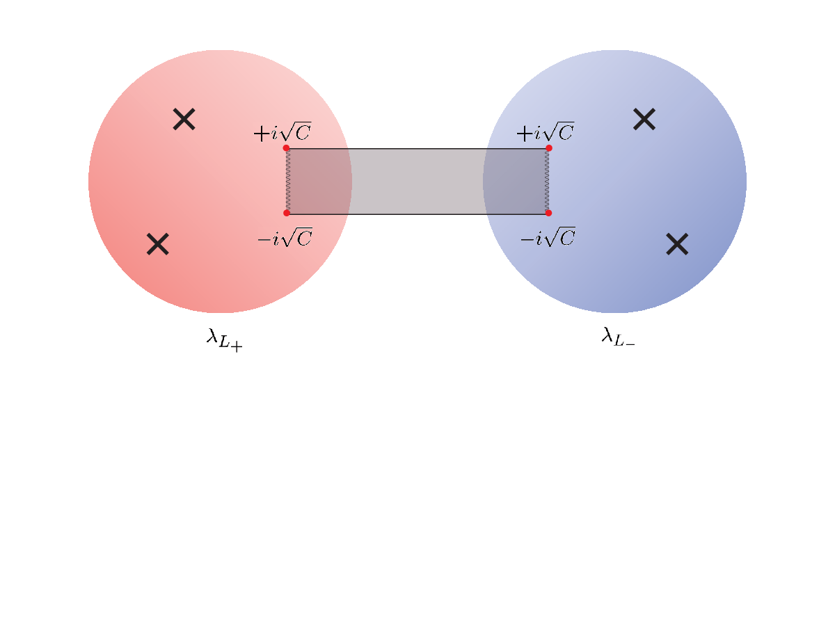
Figure 3: The λL±\lambda_{L_{\pm}}-spheres are joined on the cut between ±i​C​(C>0)\pm i\sqrt{C}~(C>0) . The constructed Riemann surface is mapped to the Riemann sphere in zRz_{R} depicted in Figure 2.

In the map (3.3) , there is a cut between +i​C+i\sqrt{C} and −i​C-i\sqrt{C} on each of the Riemann spheres with λL+\lambda_{L_{+}} and λL−\lambda_{L_{-}} , and the two Riemann spheres are joined there as depicted in Fig. 3. Then this cut corresponds to the imaginary axis of zRz_{R} . In order to see this correspondence, let us rewrite the relation (44) as

λL=i​C​1+zR21−zR2,\displaystyle\lambda_{L}=i\sqrt{C}\,\frac{1+z_{R}^{2}}{1-z_{R}^{2}}\,, (48)

and parametrize the imaginary axis of zRz_{R} as

zR=±i​e−ξ(ξ∈ℝ).\displaystyle z_{R}=\pm i\,{\rm e}^{-\xi}\qquad\left(\,\xi\in{\mathbb{R}}\,\right)\,. (49)

According to the map (48) , the imaginary axis (49) is represented by

λL=i​C​tanh⁡ξ(ξ∈ℝ)\displaystyle\lambda_{L}=i\sqrt{C}\tanh\xi\qquad\left(\,\xi\in{\mathbb{R}}\,\right) (50)

on the λL±\lambda_{L_{\pm}}-spheres. This is nothing but the cut in the map (3.3) . More precisely, depending on the sign of CC , it is written as

λL=i​y,−C<y<C(C>0),λL=x,−|C|<x<|C|(−1<C<0).\displaystyle\begin{array}[]{ccc}\lambda_{L}=iy\,,&\quad-\sqrt{C}<y<\sqrt{C}&\qquad(C>0)\,,\\ \lambda_{L}=x\,,&\quad-\sqrt{|C|}<x<\sqrt{|C|}&\qquad(-1<C<0)\,.\end{array}

Thus the resulting Riemann surface described by λL+\lambda_{L_{+}} and λL−\lambda_{L_{-}} is mapped to the Riemann sphere with zRz_{R} , each other. The number of poles is preserved under the map.

3.4 The expansions of UL±​(λL±)U^{L_{\pm}}(\lambda_{L_{\pm}}) : revisited

It is worth reconsidering the expansions of monodromy matrices with the relation (44).

As a concrete example, we will concentrate on the two expansions,

i)  UL+​(λL+)U^{L_{+}}(\lambda_{L_{+}}) around λL+=i​C\lambda_{L_{+}}=i\sqrt{C} ,
ii)  UR​(λR)U^{R}(\lambda_{R}) around zR=0z_{R}=0 .

With the relation (44) , the expansion parameter ϵ(+)+\epsilon_{(+)}^{+} in the case i) is rewritten as

ϵ(+)+=2​i​C​zR21−zR2.\displaystyle\epsilon_{(+)}^{+}=\frac{2i\sqrt{C}\,z_{R}^{2}}{1-z_{R}^{2}}\,. (54)

Since |ϵ(+)+|≪1|\epsilon_{(+)}^{+}|\ll 1 , zRz_{R} is infinitesimal. Hence ϵ(+)+\epsilon_{(+)}^{+} can be expressed as a power series in zRz_{R} .

With the relation (54) , the expansion in (36) can be rewritten as

g∞−1⋅UL+​(λL+)⋅g∞\displaystyle g_{\infty}^{-1}\cdot U^{L_{+}}(\lambda_{L_{+}})\cdot g_{\infty} (55)
=\displaystyle= e−i​γ​T3​Q(0)R,3​exp⁡[−2​i​γ​T+​eγ​Q(0)R,3/2​Q(1)R,−]\displaystyle{\rm e}^{-i\gamma T^{3}Q^{R,3}_{(0)}}\exp\left[-2i\gamma T^{+}{\rm e}^{\gamma Q^{R,3}_{(0)}/2}Q^{R,-}_{(1)}\right]
×{1−2​i​C​zR21+C[T−e−γQR,3(0)/2Q~(1)R,+−γT3[Q¯(2)R,3−Q(1)R,−Q~(1)R,+]\displaystyle\times\left\{1-\frac{2i\sqrt{C}z_{R}^{2}}{1+C}\left[T^{-}{\rm e}^{-\gamma Q^{R,3}_{(0)}/2}\widetilde{Q}^{R,+}_{(1)}-\gamma T^{3}\left[\bar{Q}^{R,3}_{(2)}-Q^{R,-}_{(1)}\widetilde{Q}^{R,+}_{(1)}\right]\right.\right.
−γ2T+eγ​Q(0)R,3/2[Q(3)R,−−Q¯(2)R,3Q(1)R,−+23(Q(1)R,−)2Q~(1)R,+]]+𝒪(zR4)}.\displaystyle\left.\left.-\gamma^{2}T^{+}{\rm e}^{\gamma Q^{R,3}_{(0)}/2}\left[Q^{R,-}_{(3)}-\bar{Q}^{R,3}_{(2)}Q^{R,-}_{(1)}+\frac{2}{3}\left(Q^{R,-}_{(1)}\right)^{2}\widetilde{Q}^{R,+}_{(1)}\right]\right]+{\mathcal{O}}(z_{R}^{4})\right\}\,.

Notice that the rescaling of s​l​(2)sl(2) generators

T±→e∓λR​T±,\displaystyle T^{\pm}~\to~{\rm e}^{\mp\lambda_{R}}\,T^{\pm}\,, (56)

makes the expansion in (55) into a significant form,

g∞−1⋅UL+​(λL+)⋅g∞\displaystyle g_{\infty}^{-1}\cdot U^{L_{+}}(\lambda_{L_{+}})\cdot g_{\infty}
=\displaystyle= e−i​γ​T3​Q(0)R,3​[1−2​i​γ​zR​T+​eγ​Q(0)R,3/2​Q(1)R,−]\displaystyle{\rm e}^{-i\gamma T^{3}Q^{R,3}_{(0)}}\left[1-2i\gamma z_{R}T^{+}{\rm e}^{\gamma Q^{R,3}_{(0)}/2}Q^{R,-}_{(1)}\right]
×{1−2iγzR2[zR−1T−e−γQR,3(0)/2Q~(1)R,+−γT3[Q¯(2)R,3−Q(1)R,−Q~(1)R,+]\displaystyle\times\left\{1-2i\gamma z_{R}^{2}\left[z_{R}^{-1}T^{-}{\rm e}^{-\gamma Q^{R,3}_{(0)}/2}\widetilde{Q}^{R,+}_{(1)}-\gamma T^{3}\left[\bar{Q}^{R,3}_{(2)}-Q^{R,-}_{(1)}\widetilde{Q}^{R,+}_{(1)}\right]\right.\right.
−γ2zRT+eγ​Q(0)R,3/2[Q(3)R,−−Q¯(2)R,3Q(1)R,−+23(Q(1)R,−)2Q~(1)R,+]]}+𝒪(zR2)\displaystyle\left.\left.-\gamma^{2}z_{R}T^{+}{\rm e}^{\gamma Q^{R,3}_{(0)}/2}\left[Q^{R,-}_{(3)}-\bar{Q}^{R,3}_{(2)}Q^{R,-}_{(1)}+\frac{2}{3}\left(Q^{R,-}_{(1)}\right)^{2}\widetilde{Q}^{R,+}_{(1)}\right]\right]\right\}+{\mathcal{O}}(z_{R}^{2})
=\displaystyle= e−i​γ​T3​Q(0)R,3{1−2iγzR[T+eγ​Q(0)R,3/2Q(1)R,−+T−e−γQR,3(0)/2Q~(1)R,+]}+𝒪(zR2).\displaystyle{\rm e}^{-i\gamma T^{3}Q^{R,3}_{(0)}}\left\{1-2i\gamma z_{R}\left[T^{+}{\rm e}^{\gamma Q^{R,3}_{(0)}/2}Q^{R,-}_{(1)}+T^{-}{\rm e}^{-\gamma Q^{R,3}_{(0)}/2}\widetilde{Q}^{R,+}_{(1)}\right]\right\}+{\mathcal{O}}(z_{R}^{2})\,.

This is nothing but the expansion in the case ii). That is, if the rescaling (56) is taken into account, then the expansion in ϵ(+)+\epsilon_{(+)}^{+} can be regarded as the one in zRz_{R} . The rescaling (56) is just an isomorphism of the s​l​(2)sl(2) algebra, hence it does not mean any modifications of the system.

Similarly, the expansion of UL+​(λL+)U^{L_{+}}(\lambda_{L_{+}}) around λL+=−i​C\lambda_{L_{+}}=-i\sqrt{C} agrees with that of UR​(λR)U^{R}(\lambda_{R}) around zR=∞z_{R}=\infty under the relation (44) with the rescaling (56). In addition, the expansion of UL−​(λL−)U^{L_{-}}(\lambda_{L_{-}}) around λL−=i​C\lambda_{L_{-}}=i\sqrt{C} (−i​C)(-i\sqrt{C}) agrees with that of UR​(λR)U^{R}(\lambda_{R}) around zR=0z_{R}=0 (∞)(\infty) , respectively, if we take another rescaling

T±→e±λR​T±.\displaystyle T^{\pm}~\rightarrow~{\rm e}^{\pm\lambda_{R}}\,T^{\pm}\,. (57)

From these agreements, one may anticipate that the rescalings of s​l​(2)sl(2) generators

T±→e∓λR​T±forUL+​(λL+),\displaystyle T^{\pm}~\to~{\rm e}^{\mp\lambda_{R}}\,T^{\pm}\qquad\mbox{for}\quad U^{L_{+}}(\lambda_{L_{+}})\,, (58)
T±→e±λR​T±forUL−​(λL−).\displaystyle T^{\pm}~\to~{\rm e}^{\pm\lambda_{R}}\,T^{\pm}\qquad\mbox{for}\quad U^{L_{-}}(\lambda_{L_{-}})\,. (59)

would be an important key in arguing the equivalence of monodromy matrices. Indeed this is the case. The rescalings will play an essential role in the next section. Note that the rescalings (58) and (59) are compatible with the sign flipping in (32) , because the shift of λR\lambda_{R} ,

λR→λR+π​i\lambda_{R}\quad\to\quad\lambda_{R}+\pi\,i

flips the sign of T±T^{\pm} after taking the rescalings (58) and (59) .

4 Gauge equivalence of monodromy matrices

Let us consider the gauge-equivalence of monodromy matrices UR​(λR)U^{R}(\lambda_{R}) and UL±​(λL±)U^{L_{\pm}}(\lambda_{L_{\pm}}) under the parameter relation (44) and the rescalings (58) and (59).

4.1 Gauge equivalence of monodromy matrices: C=0C=0

First of all, as a warming-up, we shall consider the C=0C=0 case. This is nothing but the case of S​U​(2)SU(2) principal chiral model and its classical integrability is well studied [28, 29, 30, 31, 32] (For a comprehensive book, see [33]).

On the one hand, the Lax pair in terms of the right-invariant current

jμL≡∂μg⋅g−1=g​Jμ​g−1,j^{L}_{\mu}\equiv\partial_{\mu}g\cdot g^{-1}=g\,J_{\mu}\,g^{-1}\,,

is given by

L±L​(x,λL)=11±λL​j±L,\displaystyle L^{L}_{\pm}(x;\lambda_{L})=\frac{1}{1\pm\lambda_{L}}j^{L}_{\pm}\,, (60)

where the light-cone components are defined as

LtL​(x,λL)≡12​[L+L​(x,λL)+L−L​(x,λL)],LxL​(x,λL)≡12​[L+L​(x,λL)−L−L​(x,λL)].\displaystyle L^{L}_{t}(x;\lambda_{L})\equiv\frac{1}{2}\left[L^{L}_{+}(x;\lambda_{L})+L^{L}_{-}(x;\lambda_{L})\right]\,,\quad L^{L}_{x}(x;\lambda_{L})\equiv\frac{1}{2}\left[L^{L}_{+}(x;\lambda_{L})-L^{L}_{-}(x;\lambda_{L})\right]\,.

On the other hand, the Lax pair in terms of the left-invariant current

jRμ≡−g−1∂μg=−Jμ,j^{R}_{\mu}\equiv-g^{-1}\partial_{\mu}g=-J_{\mu}\,,

is given by

L±R​(x,λR)=11±λR​j±R,\displaystyle L^{R}_{\pm}(x;\lambda_{R})=\frac{1}{1\pm\lambda_{R}}j^{R}_{\pm}\,, (61)

where the light-components are defined as

LtR​(x,λR)≡12​[L+R​(x,λR)+L−R​(x,λR)],LxR​(x,λR)≡12​[L+R​(x,λR)−L−R​(x,λR)].\displaystyle L^{R}_{t}(x;\lambda_{R})\equiv\frac{1}{2}\left[L^{R}_{+}(x;\lambda_{R})+L^{R}_{-}(x;\lambda_{R})\right]\,,\quad L^{R}_{x}(x;\lambda_{R})\equiv\frac{1}{2}\left[L^{R}_{+}(x;\lambda_{R})-L^{R}_{-}(x;\lambda_{R})\right]\,.

Then we may introduce monodromy matrices for the Lax pairs (60) and (61) like

UL​(λL)\displaystyle U^{L}(\lambda_{L}) =\displaystyle= P​exp⁡[∫−∞∞d​x​LxL​(x,λL)],\displaystyle{\rm P}\exp\left[\int^{\infty}_{-\infty}\!\!\!dxL^{L}_{x}(x;\lambda_{L})\right]\,, (62)
UR​(λR)\displaystyle U^{R}(\lambda_{R}) =\displaystyle= P​exp⁡[∫−∞∞d​x​LxR​(x,λR)].\displaystyle{\rm P}\exp\left[\int^{\infty}_{-\infty}\!\!\!dxL^{R}_{x}(x;\lambda_{R})\right]\,. (63)

From now on, we will show that the two Lax pairs (60) and (61) are gauge-equivalent under the identification of λL\lambda_{L} and λR\lambda_{R} with

λL=1λR.\displaystyle\lambda_{L}=\frac{1}{\lambda_{R}}\,. (64)

First of all, let us perform the gauge transformation for the L±L​(x,λL)L^{L}_{\pm}(x;\lambda_{L}) . Since the Lax pair is transformed as a gauge field, the transformation law is give by

[L±L​(x,λL)]g≡g−1​L±L​(x,λL)​g−g−1​∂±g=−±λL1±λL​J±.\displaystyle\Bigl[L^{L}_{\pm}(x;\lambda_{L})\Bigr]^{g}\equiv g^{-1}L^{L}_{\pm}(x;\lambda_{L})g-g^{-1}\partial_{\pm}g=-\frac{\pm\lambda_{L}}{1\pm\lambda_{L}}J_{\pm}\,. (65)

Using the relation (64) , we can show that

[L±L​(x,λL)]g=L±R​(x,λR).\displaystyle\Bigl[L^{L}_{\pm}(x;\lambda_{L})\Bigr]^{g}=L^{R}_{\pm}(x;\lambda_{R})\,. (66)

With this relation, we obtain the following formula for covariant derivatives,

g−1[∂μ−LμL(x;λL)]g=∂μ−LμR(x;λR).\displaystyle g^{-1}\left[\partial_{\mu}-L^{L}_{\mu}(x;\lambda_{L})\right]g=\partial_{\mu}-L^{R}_{\mu}(x;\lambda_{R})\,. (67)

Thus the transformation law of monodromy matrices is given by

g∞−1⋅UL​(λL)⋅g∞=UR​(λR),\displaystyle g_{\infty}^{-1}\cdot U^{L}(\lambda_{L})\cdot g_{\infty}=U^{R}(\lambda_{R})\,, (68)

and we have shown that UL​(λL)U^{L}(\lambda_{L}) is gauge-equivalent to UR​(λR)U^{R}(\lambda_{R}) under the identification (64) .

It would be interesting to see the gauge-equivalence at r/sr/s-matrix level. The r/sr/s-matrices are derived from the following Poisson brackets,

{LxL(x;λL),⊗LxL(y;μL)}P\displaystyle\left\{L^{L}_{x}(x;\lambda_{L})\stackrel{{\scriptstyle\otimes}}{{,}}L^{L}_{x}(y;\mu_{L})\right\}_{\rm P} =\displaystyle= [rL​(λL,μL),LxL​(x,λL)⊗1+1⊗LxL​(y,μL)]​δ​(x−y)\displaystyle\left[r^{L}(\lambda_{L},\mu_{L}),L^{L}_{x}(x;\lambda_{L})\otimes 1+1\otimes L^{L}_{x}(y;\mu_{L})\right]\delta(x-y)
−[sL​(λL,μL),LxL​(x,λL)⊗1−1⊗LxL​(y,μL)]​δ​(x−y)\displaystyle-\left[s^{L}(\lambda_{L},\mu_{L}),L^{L}_{x}(x;\lambda_{L})\otimes 1-1\otimes L^{L}_{x}(y;\mu_{L})\right]\delta(x-y)
−2sL(λL,μL)∂xδ(x−y),\displaystyle-2s^{L}(\lambda_{L},\mu_{L})\partial_{x}\delta(x-y)\,,
{LxR(x;λR),⊗LxR(y;μR)}P\displaystyle\left\{L^{R}_{x}(x;\lambda_{R})\stackrel{{\scriptstyle\otimes}}{{,}}L^{R}_{x}(y;\mu_{R})\right\}_{\rm P} =\displaystyle= [rR​(λR,μR),LxR​(x,λR)⊗1+1⊗LxR​(y,μR)]​δ​(x−y)\displaystyle\left[r^{R}(\lambda_{R},\mu_{R}),L^{R}_{x}(x;\lambda_{R})\otimes 1+1\otimes L^{R}_{x}(y;\mu_{R})\right]\delta(x-y)
−[sR​(λR,μR),LxR​(x,λR)⊗1−1⊗LxR​(y,μR)]​δ​(x−y)\displaystyle-\left[s^{R}(\lambda_{R},\mu_{R}),L^{R}_{x}(x;\lambda_{R})\otimes 1-1\otimes L^{R}_{x}(y;\mu_{R})\right]\delta(x-y)
−2sR(λR,μR)∂xδ(x−y).\displaystyle-2s^{R}(\lambda_{R},\mu_{R})\partial_{x}\delta(x-y)\,.

The classical r/sr/s-matrices are the following:

rL​(λL,μL)=h⁡(λL)+h⁡(μL)2​(λL−μL)​(T+⊗T−+T−⊗T++T3⊗T3),\displaystyle r^{L}(\lambda_{L},\mu_{L})=\frac{h(\lambda_{L})+h(\mu_{L})}{2\left(\lambda_{L}-\mu_{L}\right)}\left(T^{+}\otimes T^{-}+T^{-}\otimes T^{+}+T^{3}\otimes T^{3}\right)\,,
sL​(λL,μL)=h⁡(λL)−h⁡(μL)2​(λL−μL)​(T+⊗T−+T−⊗T++T3⊗T3),\displaystyle s^{L}(\lambda_{L},\mu_{L})=\frac{h(\lambda_{L})-h(\mu_{L})}{2\left(\lambda_{L}-\mu_{L}\right)}\left(T^{+}\otimes T^{-}+T^{-}\otimes T^{+}+T^{3}\otimes T^{3}\right)\,,
rR​(λR,μR)=h⁡(λR)+h⁡(μR)2​(λR−μR)​(T+⊗T−+T−⊗T++T3⊗T3),\displaystyle r^{R}(\lambda_{R},\mu_{R})=\frac{h(\lambda_{R})+h(\mu_{R})}{2\left(\lambda_{R}-\mu_{R}\right)}\left(T^{+}\otimes T^{-}+T^{-}\otimes T^{+}+T^{3}\otimes T^{3}\right)\,,
sR​(λR,μR)=h⁡(λR)−h⁡(μR)2​(λR−μR)​(T+⊗T−+T−⊗T++T3⊗T3).\displaystyle s^{R}(\lambda_{R},\mu_{R})=\frac{h(\lambda_{R})-h(\mu_{R})}{2\left(\lambda_{R}-\mu_{R}\right)}\left(T^{+}\otimes T^{-}+T^{-}\otimes T^{+}+T^{3}\otimes T^{3}\right)\,. (69)

Here h⁡(λ)h(\lambda) is defined as

h⁡(λ)≡λ21−λ2.\displaystyle h(\lambda)\equiv\frac{\lambda^{2}}{1-\lambda^{2}}\,. (70)

It is straightforward to compute the gauge transformation laws of r/sr/s-matrices. The rr-matrix is transformed as

[rL​(λL,μL)​δ​(x−y)]g\displaystyle\Bigl[r^{L}(\lambda_{L},\mu_{L})\delta(x-y)\Bigr]^{g} =\displaystyle= g−1(x)⊗g−1(y)[rL(λL,μL)δ(x−y)\displaystyle g^{-1}(x)\otimes g^{-1}(y)\left[r^{L}(\lambda_{L},\mu_{L})\delta(x-y)\right.
−12{g(x),⊗LxL(y;μL)}Pg−1(x)⊗1\displaystyle-\left.\frac{1}{2}\left\{g(x)\stackrel{{\scriptstyle\otimes}}{{,}}L^{L}_{x}(y;\mu_{L})\right\}_{\rm P}g^{-1}(x)\otimes 1\right.
−12{LxL(x;λL),⊗g(y)}P1⊗g−1(y)]g(x)⊗g(y),\displaystyle\left.-\frac{1}{2}\left\{L^{L}_{x}(x;\lambda_{L})\stackrel{{\scriptstyle\otimes}}{{,}}g(y)\right\}_{\rm P}1\otimes g^{-1}(y)\right]g(x)\otimes g(y)\,,

and the ss-matrix is transformed as

[sL​(λL,μL)​δ​(x−y)]g\displaystyle\Bigl[s^{L}(\lambda_{L},\mu_{L})\delta(x-y)\Bigr]^{g} =\displaystyle= g−1(x)⊗g−1(y)[sL(λL,μL)δ(x−y)\displaystyle g^{-1}(x)\otimes g^{-1}(y)\left[s^{L}(\lambda_{L},\mu_{L})\delta(x-y)\right.
+12{g(x),⊗LxL(y;μL)}Pg−1(x)⊗1\displaystyle\left.+\frac{1}{2}\left\{g(x)\stackrel{{\scriptstyle\otimes}}{{,}}L^{L}_{x}(y;\mu_{L})\right\}_{\rm P}g^{-1}(x)\otimes 1\right.
−12{LxL(x;λL),⊗g(y)}P1⊗g−1(y)]g(x)⊗g(y).\displaystyle\left.-\frac{1}{2}\left\{L^{L}_{x}(x;\lambda_{L})\stackrel{{\scriptstyle\otimes}}{{,}}g(y)\right\}_{\rm P}1\otimes g^{-1}(y)\right]g(x)\otimes g(y)\,.

With the Poisson brackets,

{g(x),⊗LxL(y;μL)}P=μLμL2−1(T+⊗T−+T−⊗T++T3⊗T3)g(x)⊗1δ(x−y),\displaystyle\left\{g(x)\stackrel{{\scriptstyle\otimes}}{{,}}L^{L}_{x}(y;\mu_{L})\right\}_{\rm P}=\frac{\mu_{L}}{\mu_{L}^{2}-1}\left(T^{+}\otimes T^{-}+T^{-}\otimes T^{+}+T^{3}\otimes T^{3}\right)g(x)\otimes 1\delta(x-y)\,,
{LxL(x;λL),⊗g(y)}P=−λLλL2−1(T+⊗T−+T−⊗T++T3⊗T3)1⊗g(y)δ(x−y).\displaystyle\left\{L^{L}_{x}(x;\lambda_{L})\stackrel{{\scriptstyle\otimes}}{{,}}g(y)\right\}_{\rm P}=-\frac{\lambda_{L}}{\lambda_{L}^{2}-1}\left(T^{+}\otimes T^{-}+T^{-}\otimes T^{+}+T^{3}\otimes T^{3}\right)1\otimes g(y)\delta(x-y)\,.

the gauge-equivalence of r/sr/s-matrices are shown as

[rL​(λL,μL)]g=rR​(λR,μR),[sL​(λL,μL)]g=sR​(λR,μR).\displaystyle\Bigl[r^{L}(\lambda_{L},\mu_{L})\Bigr]^{g}=r^{R}(\lambda_{R},\mu_{R})\,,\qquad\Bigl[s^{L}(\lambda_{L},\mu_{L})\Bigr]^{g}=s^{R}(\lambda_{R},\mu_{R})\,.

This equivalence still holds even after squashing the target space geometry, as we will see in the next subsection.

Finally we should emphasize the advantage of r/sr/s-matrix formalism. If one uses the retarded monodromy matrix in [24], instead of the r/sr/s-matrix formalism, then the gauge-equivalence does not hold.

4.2 Gauge equivalence of monodromy matrices: C≠0C\neq 0

It is a turn to consider the squashed sigma model case with C≠0C\neq 0 . Here we will show that UR​(λR)U^{R}(\lambda_{R}) is gauge-equivalent to UL±​(λL±)U^{L_{\pm}}(\lambda_{L_{\pm}}) under the relation (44) and the rescalings (58) and (59) .

Let us start from rewriting the Lax pair L±L+​(x,λL+)L_{\pm}^{L_{+}}(x;\lambda_{L_{+}}) as

L±L+​(x,λL+)\displaystyle L^{L_{+}}_{\pm}(x;\lambda_{L_{+}})
=\displaystyle= 11±λL+​g​[T+​(1∓i​C)​J±−+T−​(1±i​C)​J±++T3​(1+C)​J±3]​g−1.\displaystyle\frac{1}{1\pm\lambda_{L_{+}}}g\left[T^{+}\!\left(1\mp i\sqrt{C}\right)\!J^{-}_{\pm}\!+\!T^{-}\!\left(1\pm i\sqrt{C}\right)\!J^{+}_{\pm}\!+\!T^{3}\!\left(1+C\right)\!J^{3}_{\pm}\right]g^{-1}\,.

As in the case with C=0C=0 , a gauge transformation of it is evaluated as

[L±L+​(x,λL+)]g≡g−1​L±L+​(x,λL+)​g−g−1​∂±g\displaystyle\Bigl[L^{L_{+}}_{\pm}(x;\lambda_{L_{+}})\Bigr]^{g}\equiv g^{-1}L^{L_{+}}_{\pm}(x;\lambda_{L_{+}})g-g^{-1}\partial_{\pm}g
=\displaystyle= −J±+11±λL+​[T+​(1∓i​C)​J±−+T−​(1±i​C)​J±++T3​(1+C)​J±3]\displaystyle-J_{\pm}+\frac{1}{1\pm\lambda_{L_{+}}}\left[T^{+}\!\left(1\mp i\sqrt{C}\right)\!J^{-}_{\pm}\!+\!T^{-}\!\left(1\pm i\sqrt{C}\right)\!J^{+}_{\pm}\!+\!T^{3}\!\left(1+C\right)\!J^{3}_{\pm}\right]
=\displaystyle= −±λL+1±λL+​[T+​(1+i​CλL+)​J±−+T−​(1−i​CλL+)​J±++T3​(1∓CλL+)​J±3].\displaystyle-\frac{\pm\lambda_{L_{+}}}{1\pm\lambda_{L_{+}}}\left[T^{+}\!\left(1+\frac{i\sqrt{C}}{\lambda_{L_{+}}}\right)\!J^{-}_{\pm}\!+\!T^{-}\!\left(1-\frac{i\sqrt{C}}{\lambda_{L_{+}}}\right)\!J^{+}_{\pm}\!+\!T^{3}\!\left(1\mp\frac{C}{\lambda_{L_{+}}}\right)\!J^{3}_{\pm}\right]\,.

By using the inverse relation of (44) ,

λL±=tanh⁡αtanh⁡λR,\displaystyle\lambda_{L_{\pm}}=\frac{\tanh\alpha}{\tanh\lambda_{R}}\,, (71)

the gauge transformation is further rewritten as

[L±L+​(x,λL+)]g=−sinh⁡αsinh⁡(α±λR)​[T+​eλR​J±−+T−​e−λR​J±++T3​cosh⁡(α±λR)cosh⁡α​J±3].\displaystyle\Bigl[L^{L_{+}}_{\pm}(x;\lambda_{L_{+}})\Bigr]^{g}=-\frac{\sinh\alpha}{\sinh(\alpha\pm\lambda_{R})}\left[T^{+}{\rm e}^{\lambda_{R}}J^{-}_{\pm}\!+\!T^{-}{\rm e}^{-\lambda_{R}}J^{+}_{\pm}\!+\!T^{3}\frac{\cosh(\alpha\pm\lambda_{R})}{\cosh\alpha}J^{3}_{\pm}\right]\,.

Thus, up to the rescaling (58), we have shown that

[L±L+​(x,λL+)]g≃L±R​(x,λR).\displaystyle\Bigl[L^{L_{+}}_{\pm}(x;\lambda_{L_{+}})\Bigr]^{g}\simeq L^{R}_{\pm}(x;\lambda_{R})\,. (72)

This relation means the gauge-equivalence of monodromy matrices,

g∞−1⋅UL+​(λL+)⋅g∞≃UR​(λR).\displaystyle g_{\infty}^{-1}\cdot U^{L_{+}}(\lambda_{L_{+}})\cdot g_{\infty}\simeq U^{R}(\lambda_{R})\,. (73)

Note that only half of the range of λR\lambda_{R} is covered by λL+\lambda_{L_{+}} , as we know from (3.3) .

The same argument is possible for UL−​(λL−)U^{L_{-}}(\lambda_{L_{-}}) . Only the difference is that the rescaling (59) has to be used instead of (58) . Then we obtain that

g∞−1⋅UL−​(λL−)⋅g∞≃UR​(λR).\displaystyle g_{\infty}^{-1}\cdot U^{L_{-}}(\lambda_{L_{-}})\cdot g_{\infty}\simeq U^{R}(\lambda_{R})\,. (74)

The remaining range of λR\lambda_{R} is covered by λ−\lambda_{-} . Thus, putting (73) and (74) together, we have shown that UR​(λR)U^{R}(\lambda_{R}) is gauge-equivalent to UL±​(λL±)U^{L_{\pm}}(\lambda_{L_{\pm}}) .

Let us comment on the rescalings (58) and (59) . They can be expressed as a transformation generated by e∓i​T3​λR{\rm e}^{\mp iT^{3}\lambda_{R}} . Then the Lax pair is transformed as

LμR±​(x,λR)=e±i​T3​λR​LμR​(x,λR)​e∓i​T3​λR.\displaystyle L^{R_{\pm}}_{\mu}(x;\lambda_{R})={\rm e}^{\pm iT^{3}\lambda_{R}}\,L^{R}_{\mu}(x;\lambda_{R})\,{\rm e}^{\mp iT^{3}\lambda_{R}}\,. (75)

With this transformation law, the gauge-equivalence of monodromy matrices is represented by a simple form,

g~±−1⋅UL±​(λL±)⋅g~±=UR​(λR),g~±≡g∞⋅e±i​T3​λR.\displaystyle\widetilde{g}_{\pm}^{-1}\cdot U^{L_{\pm}}(\lambda_{L_{\pm}})\cdot\widetilde{g}_{\pm}=U^{R}(\lambda_{R})\,,\qquad\widetilde{g}_{\pm}\equiv g_{\infty}\cdot{\rm e}^{\pm iT^{3}\lambda_{R}}\,. (76)

Note that λR\lambda_{R} is a complex variable and hence the transformation (75) is not an S​U​(2)LSU(2)_{\rm L} transformation.

The next task is to check the gauge-equivalence at the r/sr/s-matrix level. Recall that the left and right r/sr/s-matrices are given by [18]

rL±​(λL±,μL±)=hL​(λL±)+hL​(μL±)2​(λL±−μL±)​(T+⊗T−+T−⊗T++T3⊗T3),\displaystyle r^{L_{\pm}}(\lambda_{L_{\pm}},\mu_{L_{\pm}})=\frac{h^{L}(\lambda_{L_{\pm}})+h^{L}(\mu_{L_{\pm}})}{2\left(\lambda_{L_{\pm}}-\mu_{L_{\pm}}\right)}\left(T^{+}\otimes T^{-}+T^{-}\otimes T^{+}+T^{3}\otimes T^{3}\right)\,,
sL±​(λL±,μL±)=hL​(λL±)−hL​(μL±)2​(λL±−μL±)​(T+⊗T−+T−⊗T++T3⊗T3),\displaystyle s^{L_{\pm}}(\lambda_{L_{\pm}},\mu_{L_{\pm}})=\frac{h^{L}(\lambda_{L_{\pm}})-h^{L}(\mu_{L_{\pm}})}{2\left(\lambda_{L_{\pm}}-\mu_{L_{\pm}}\right)}\left(T^{+}\otimes T^{-}+T^{-}\otimes T^{+}+T^{3}\otimes T^{3}\right)\,,
rR​(λR,μR)=hR​(λR)+hR​(μR)2​sinh⁡(λR−μR)​(T+⊗T−+T−⊗T++cosh⁡(λR−μR)​T3⊗T3),\displaystyle r^{R}(\lambda_{R},\mu_{R})=\frac{h^{R}(\lambda_{R})+h^{R}(\mu_{R})}{2\sinh\left(\lambda_{R}-\mu_{R}\right)}\left(T^{+}\otimes T^{-}+T^{-}\otimes T^{+}+\cosh\left(\lambda_{R}-\mu_{R}\right)T^{3}\otimes T^{3}\right)\,,
sR​(λR,μR)=hR​(λR)−hR​(μR)2​sinh⁡(λR−μR)​(T+⊗T−+T−⊗T++cosh⁡(λR−μR)​T3⊗T3).\displaystyle s^{R}(\lambda_{R},\mu_{R})=\frac{h^{R}(\lambda_{R})-h^{R}(\mu_{R})}{2\sinh\left(\lambda_{R}-\mu_{R}\right)}\left(T^{+}\otimes T^{-}+T^{-}\otimes T^{+}+\cosh\left(\lambda_{R}-\mu_{R}\right)T^{3}\otimes T^{3}\right)\,.

Here scalar functions hL​(λL)h^{L}(\lambda_{L}) and hR​(λR)h^{R}(\lambda_{R}) are defined as, respectively,

hL​(λL)\displaystyle h^{L}(\lambda_{L}) ≡\displaystyle\equiv C+λL21−λL2,\displaystyle\frac{C+\lambda_{L}^{2}}{1-\lambda_{L}^{2}}\,, (77)
hR​(λR)\displaystyle h^{R}(\lambda_{R}) ≡\displaystyle\equiv sinh⁡α​cosh⁡α​sinh2⁡λRsinh⁡(α−λR)​sinh⁡(α+λR).\displaystyle\frac{\sinh\alpha\cosh\alpha\sinh^{2}\lambda_{R}}{\sinh(\alpha-\lambda_{R})\sinh(\alpha+\lambda_{R})}\,. (78)

Under the gauge transformation, the rational r/sr/s-matrices are transformed as

[rL±​(λL±,μL±)​δ​(x−y)]g\displaystyle\Bigl[r^{L_{\pm}}(\lambda_{L_{\pm}},\mu_{L_{\pm}})\delta(x-y)\Bigr]^{g}
=\displaystyle= g−1(x)⊗g−1(y)[rL±(λL±,μL±)δ(x−y)−12{g(x),⊗LxL±(y;μL±)}Pg−1(x)⊗1\displaystyle g^{-1}(x)\otimes g^{-1}(y)\left[r^{L_{\pm}}(\lambda_{L_{\pm}},\mu_{L_{\pm}})\delta(x-y)-\frac{1}{2}\left\{g(x)\stackrel{{\scriptstyle\otimes}}{{,}}L^{L_{\pm}}_{x}(y;\mu_{L_{\pm}})\right\}_{\rm P}g^{-1}(x)\otimes 1\right.
−12{LxL±(x;λL±),⊗g(y)}P1⊗g−1(y)]g(x)⊗g(y)\displaystyle\qquad\qquad\qquad\qquad\left.-\frac{1}{2}\left\{L^{L_{\pm}}_{x}(x;\lambda_{L_{\pm}})\stackrel{{\scriptstyle\otimes}}{{,}}g(y)\right\}_{\rm P}1\otimes g^{-1}(y)\right]g(x)\otimes g(y)
[sL±​(λL±,μL±)​δ​(x−y)]g\displaystyle\Bigl[s^{L_{\pm}}(\lambda_{L_{\pm}},\mu_{L_{\pm}})\delta(x-y)\Bigr]^{g}
=\displaystyle= g−1(x)⊗g−1(y)[sL±(λL±,μL±)δ(x−y)+12{g(x),⊗LxL±(y;μL±)}Pg−1(x)⊗1\displaystyle g^{-1}(x)\otimes g^{-1}(y)\left[s^{L_{\pm}}(\lambda_{L_{\pm}},\mu_{L_{\pm}})\delta(x-y)+\frac{1}{2}\left\{g(x)\stackrel{{\scriptstyle\otimes}}{{,}}L^{L_{\pm}}_{x}(y;\mu_{L_{\pm}})\right\}_{\rm P}g^{-1}(x)\otimes 1\right.
−12{LxL±(x;λL±),⊗g(y)}P1⊗g−1(y)]g(x)⊗g(y).\displaystyle\qquad\qquad\qquad\qquad\left.-\frac{1}{2}\left\{L^{L_{\pm}}_{x}(x;\lambda_{L_{\pm}})\stackrel{{\scriptstyle\otimes}}{{,}}g(y)\right\}_{\rm P}1\otimes g^{-1}(y)\right]g(x)\otimes g(y)\,.

By using the following Poisson brackets,

{g(x),⊗LxL±(y;μL)}P\displaystyle\left\{g(x)\stackrel{{\scriptstyle\otimes}}{{,}}L^{L_{\pm}}_{x}(y;\mu_{L})\right\}_{\rm P} (79)
=\displaystyle= {−μL1−μL2(T+⊗T−+T−⊗T++T3⊗T3)\displaystyle\left\{\frac{-\mu_{L}}{1-\mu_{L}^{2}}\left(T^{+}\!\otimes\!T^{-}+T^{-}\!\otimes\!T^{+}+T^{3}\!\otimes\!T^{3}\right)\right.
±C1−μL2[T+⊗T−+T−⊗T++T3⊗T3,gT3g−1(x)⊗1]}g(x)⊗1δ(x−y),\displaystyle\pm\left.\frac{\sqrt{C}}{1-\mu_{L}^{2}}\left[T^{+}\!\otimes\!T^{-}+T^{-}\!\otimes\!T^{+}+T^{3}\!\otimes\!T^{3},gT^{3}g^{-1}(x)\!\otimes\!1\right]\right\}g(x)\!\otimes\!1\delta(x-y)\,,
{LxL±(x;λL),⊗g(y)}P\displaystyle\left\{L^{L_{\pm}}_{x}(x;\lambda_{L})\stackrel{{\scriptstyle\otimes}}{{,}}g(y)\right\}_{\rm P} (80)
=\displaystyle= {λL1−λL2(T+⊗T−+T−⊗T++T3⊗T3)\displaystyle\left\{\frac{\lambda_{L}}{1-\lambda_{L}^{2}}\left(T^{+}\!\otimes\!T^{-}+T^{-}\!\otimes\!T^{+}+T^{3}\!\otimes\!T^{3}\right)\right.
∓C1−λL2[T+⊗T−+T−⊗T++T3⊗T3,⊗gT3g−1(y)]}⊗g(y)δ(x−y),\displaystyle\mp\left.\frac{\sqrt{C}}{1-\lambda_{L}^{2}}\left[T^{+}\!\otimes\!T^{-}+T^{-}\!\otimes\!T^{+}+T^{3}\!\otimes\!T^{3},1\!\otimes\!gT^{3}g^{-1}(y)\right]\right\}1\!\otimes\!g(y)\delta(x-y)\,,

and the rescalings (58) and (59) , the gauge-equivalence of rr/ss-matrices are shown as

[rL±​(λL±,μL±)]g≃rR​(λR,μR),[sL±​(λL±,μL±)]g≃sR​(λR,μR).\displaystyle\Bigl[r^{L_{\pm}}(\lambda_{L_{\pm}},\mu_{L_{\pm}})\Bigr]^{g}\simeq r^{R}(\lambda_{R},\mu_{R})\,,\qquad\Bigl[s^{L_{\pm}}(\lambda_{L_{\pm}},\mu_{L_{\pm}})\Bigr]^{g}\simeq s^{R}(\lambda_{R},\mu_{R})\,.

At first glance, it might seem contradictory because the number of poles of hL​(λL)h^{L}(\lambda_{L}) is two and that of hR​(λR)h^{R}(\lambda_{R}) is four. However, the map (3.3) means that the range of λR\lambda_{R} is divided into the two regions, hence the number of poles is also compatible. This is the case for the pole of rr-matrix apart from those in hL​(λL)h^{L}(\lambda_{L}) and hR​(λR)h^{R}(\lambda_{R}) . Its number is just one and exactly agrees with the number in either of the rational descriptions.

Finally we should comment on the C→0C\to 0 limit. The relation (71) is reduced to the relation (64) in the C→0C\rightarrow 0 limit with the rescaling (9).

4.3 Reduced trigonometric description and integrability

In the previous argument, one may have noticed the possibility that a couple of the two Lax pairs

L±R+​(x,λR+)\displaystyle L^{R_{+}}_{\pm}(x;\lambda_{R_{+}}) (81)
=\displaystyle= −sinh⁡αsinh⁡(α±λR+)​[e−λR+​T−​J±++eλR+​T+​J±−+cosh⁡(α±λR+)cosh⁡α​T3​J±3],\displaystyle-\frac{\sinh\alpha}{\sinh\left(\alpha\pm\lambda_{R_{+}}\right)}\left[{\rm e}^{-\lambda_{R_{+}}}T^{-}J^{+}_{\pm}+{\rm e}^{\lambda_{R_{+}}}T^{+}J^{-}_{\pm}+\frac{\cosh\left(\alpha\pm\lambda_{R_{+}}\right)}{\cosh\alpha}T^{3}J^{3}_{\pm}\right]\,,
L±R−​(x,λR−)\displaystyle L^{R_{-}}_{\pm}(x;\lambda_{R_{-}})
=\displaystyle= −sinh⁡αsinh⁡(α±λR−)​[eλR−​T−​J±++e−λR−​T+​J±−+cosh⁡(α±λR−)cosh⁡α​T3​J±3],\displaystyle-\frac{\sinh\alpha}{\sinh\left(\alpha\pm\lambda_{R_{-}}\right)}\left[{\rm e}^{\lambda_{R_{-}}}T^{-}J^{+}_{\pm}+{\rm e}^{-\lambda_{R_{-}}}T^{+}J^{-}_{\pm}+\frac{\cosh\left(\alpha\pm\lambda_{R_{-}}\right)}{\cosh\alpha}T^{3}J^{3}_{\pm}\right]\,,

are available in the trigonometric description, instead of the Lax pair LμR​(x,λR)L^{R}_{\mu}(x;\lambda_{R}) in (6) . Now that two spectral parameters λR±\lambda_{R_{\pm}} are contained in the Lax pairs (81), the periodicity of Im​λR±{\rm Im}\,\lambda_{R_{\pm}} is π\pi, not 2​π2\pi :

LμR±​(x,λR±+π​i)=LμR±​(x,λR±).\displaystyle L^{R_{\pm}}_{\mu}(x;\lambda_{R_{\pm}}\!+\pi i)=L^{R_{\pm}}_{\mu}(x;\lambda_{R_{\pm}})\,. (82)

This observation implies that the Lax pair (6) is “reducible” in some sense. In fact, it is straightforward to check that each of the Lax pairs (81) leads to the identical classical equations of motion (5). Hence it really works well as the Lax pair, at least, at the classical level, though it is unclear whether it works even at the quantum level or not.

The two spectral parameters decompose the relation (44) into the two relations,

λL±=tanh⁡αtanh⁡λR±.\displaystyle\lambda_{L_{\pm}}=\frac{\tanh\alpha}{\tanh\lambda_{R_{\pm}}}\,. (83)

With the relation (83) , a gauge-transformation of L±L+​(x,λL+)L^{L_{+}}_{\pm}(x;\lambda_{L_{+}}) can be shown as

[L±L+​(x,λL+)]g=g−1​L±L+​(x,λL+)​g−g−1​∂±g\displaystyle\Bigl[L^{L_{+}}_{\pm}(x;\lambda_{L_{+}})\Bigr]^{g}=g^{-1}L^{L_{+}}_{\pm}(x;\lambda_{L_{+}})g-g^{-1}\partial_{\pm}g (84)
=\displaystyle= −±λL+1±λL+​[T+​(1+i​CλL+)​J±−+T−​(1−i​CλL+)​J±++T3​(1∓CλL+)​J±3]\displaystyle-\frac{\pm\lambda_{L_{+}}}{1\pm\lambda_{L_{+}}}\left[T^{+}\!\left(1+\frac{i\sqrt{C}}{\lambda_{L_{+}}}\right)\!J^{-}_{\pm}\!+\!T^{-}\!\left(1-\frac{i\sqrt{C}}{\lambda_{L_{+}}}\right)\!J^{+}_{\pm}\!+\!T^{3}\!\left(1\mp\frac{C}{\lambda_{L_{+}}}\right)\!J^{3}_{\pm}\right]
=\displaystyle= −sinh⁡αsinh⁡(α±λR+)​[T+​eλR+​J±−+T−​e−λR+​J±++T3​cosh⁡(α±λR+)cosh⁡α​J±3]\displaystyle-\frac{\sinh\alpha}{\sinh(\alpha\pm\lambda_{R_{+}})}\left[T^{+}{\rm e}^{\lambda_{R_{+}}}J^{-}_{\pm}\!+\!T^{-}{\rm e}^{-\lambda_{R_{+}}}J^{+}_{\pm}\!+\!T^{3}\frac{\cosh(\alpha\pm\lambda_{R_{+}})}{\cosh\alpha}J^{3}_{\pm}\right]
=\displaystyle= L±R+​(x,λR+).\displaystyle L^{R_{+}}_{\pm}(x;\lambda_{R_{+}})\,.

Thus we have shown the gauge-equivalence as

[L±L+​(x,λL+)]g=L±R+​(x,λR+),\displaystyle\Bigl[L^{L_{+}}_{\pm}(x;\lambda_{L_{+}})\Bigr]^{g}=L^{R_{+}}_{\pm}(x;\lambda_{R_{+}})\,, (85)

without the rescalings of s​l​(2)sl(2) generators. The gauge-equivalence of L±L−​(x,λL−)L^{L_{-}}_{\pm}(x;\lambda_{L_{-}}) and L±R−​(x,λR−)L^{R_{-}}_{\pm}(x;\lambda_{R_{-}}) can also be shown in the same way.

To summarize, the monodromy matrices satisfy the relations,

g∞−1⋅UL±​(λL±)⋅g∞=UR±​(λR±).\displaystyle g_{\infty}^{-1}\cdot U^{L_{\pm}}(\lambda_{L_{\pm}})\cdot g_{\infty}=U^{R_{\pm}}(\lambda_{R_{\pm}})\,. (86)

The next is to consider the r/sr/s-matrices related to a pair of the Lax pairs (81) . From the Poisson brackets of the spatial components of the Lax pairs (81) , similarly, one can read off the r/sr/s-matrices,

rR±​(λR±,μR±)=hR​(λR±)+hR​(μR±)2​sinh⁡(λR±−μR±)​(e±(λR±−μR±)​T+⊗T−CLOSE\displaystyle r^{R_{\pm}}(\lambda_{R_{\pm}},\mu_{R_{\pm}})=\frac{h^{R}(\lambda_{R_{\pm}})+h^{R}(\mu_{R_{\pm}})}{2\sinh\left(\lambda_{R_{\pm}}-\mu_{R_{\pm}}\right)}\left({\rm e}^{\pm\left(\lambda_{R_{\pm}}-\mu_{R_{\pm}}\right)}T^{+}\otimes T^{-}\right.
+e∓(λR±−μR±)T−⊗T++cosh(λR±−μR±)T3⊗T3),\displaystyle\hskip 85.35826pt\left.+{\rm e}^{\mp\left(\lambda_{R_{\pm}}-\mu_{R_{\pm}}\right)}T^{-}\otimes T^{+}+\cosh\left(\lambda_{R_{\pm}}-\mu_{R_{\pm}}\right)T^{3}\otimes T^{3}\right)\,, (87)
sR±​(λR±,μR±)=hR​(λR±)−hR​(μR±)2​sinh⁡(λR±−μR±)​(e±(λR±−μR±)​T+⊗T−CLOSE\displaystyle s^{R_{\pm}}(\lambda_{R_{\pm}},\mu_{R_{\pm}})=\frac{h^{R}(\lambda_{R_{\pm}})-h^{R}(\mu_{R_{\pm}})}{2\sinh\left(\lambda_{R_{\pm}}-\mu_{R_{\pm}}\right)}\left({\rm e}^{\pm\left(\lambda_{R_{\pm}}-\mu_{R_{\pm}}\right)}T^{+}\otimes T^{-}\right.
+e∓(λR±−μR±)T−⊗T++cosh(λR±−μR±)T3⊗T3).\displaystyle\hskip 85.35826pt\left.+{\rm e}^{\mp\left(\lambda_{R_{\pm}}-\mu_{R_{\pm}}\right)}T^{-}\otimes T^{+}+\cosh\left(\lambda_{R_{\pm}}-\mu_{R_{\pm}}\right)T^{3}\otimes T^{3}\right)\,. (88)

Here a scalar function hR​(λR±)h^{R}(\lambda_{R_{\pm}}) is already introduced in (78). The r/sr/s-matrices satisfy the extended Yang-Baxter equation (16), and the classical integrability has also been shown based on the Lax pair (81) .

Note that the range of λR±\lambda_{R_{\pm}} is restricted to half of the original trigonometric one as in (82) . So the number of poles in hR​(λR±)h^{R}(\lambda_{R_{\pm}}) is just two and it agrees with that in either of the rational descriptions. This is the case for the poles of the rr-matrix apart from the poles in hR​(λR±)h^{R}(\lambda_{R_{\pm}}) and it is just one. Thus the rr-matrix is really of rational type in the sense of [25], though it does not look so.

This can be confirmed by showing that the r/sr/s-matrices in the rational and reduced trigonometric descriptions are related each other by a gauge transformation. The Poisson brackets (79) and (80) lead to the transformation laws

[rL±​(λL±,μL±)​δ​(x−y)]g=rR±​(λR±,μR±)​δ​(x−y),\displaystyle\Bigl[r^{L_{\pm}}(\lambda_{L_{\pm}},\mu_{L_{\pm}})\delta(x-y)\Bigr]^{g}=r^{R_{\pm}}(\lambda_{R_{\pm}},\mu_{R_{\pm}})\delta(x-y)\,, (89)
[sL±​(λL±,μL±)​δ​(x−y)]g=sR±​(λR±,μR±)​δ​(x−y),\displaystyle\Bigl[s^{L_{\pm}}(\lambda_{L_{\pm}},\mu_{L_{\pm}})\delta(x-y)\Bigr]^{g}=s^{R_{\pm}}(\lambda_{R_{\pm}},\mu_{R_{\pm}})\delta(x-y)\,, (90)

without rescaling the s​l​(2)sl(2) generators. The relations (89) and (90) confirm that the r/sr/s-matrices (87) and (88) should be regarded as those of rational type.

Thus the trigonometric Lax pair (6) is really reducible to a pair of the rational Lax pairs (81) applicable to the classical analysis of the squashed sigma models. It would be interesting to consider how to interpret the reducibility of the Lax pair (6), at the quantum level, especially in the language of Bethe ansatz [22, 34, 35, 36, 37].

5 Conclusion and discussion

We have shown the gauge-equivalence of monodromy matrices in the trigonometric and rational descriptions under the relation of spectral parameters and the rescalings of s​l​(2)sl(2) generators. As a result, the trigonometric description has been shown to be equivalent to a pair of the rational descriptions. That is, the “global” equivalence is accurately realized even after squashing the target space geometry. Moreover, we have found the trigonometric description is reducible to a pair of the “reduced” trigonometric descriptions, each of which is of rational class and works well as the Lax pair at the classical level. With this description, the equivalence of monodromy matrices has become very apparent.

The equivalence implies that a squashed sphere is represented by a pair of round spheres as a dipole from the viewpoint of classical integrability. This is equivalent to say that a warped AdS3 space is a pair of undeformed AdS3 spaces via a double Wick rotation. This dipole-like structure of target space would correspond to that of dipole CFT2 in warped AdS3/CFT2 [12, 13]. It is a challenging issue to try to establish the correspondence in the scenario.

In this direction the rational description would play an important role based on the “global” equivalence because a Virasoro symmetry is realized as a reprametrization of the initial data in the solution generating techniques, as dicussed in [38, 39, 40]. This Virasoro symmetry is different from the one coming from the classical conformal symmetry of the system. Thus we speculate that the former Virasoro algebra and the initial data can be related to the quantities in the conjectured dual “dipole CFT” [12, 13]. This scenario might give a successful way to identify the dual CFT at the sigma model level, while the asymptotic symmetry analysis at the gravity level has not completely succeeded so far. Similarly, the related Kac-Moody algebra can also be discussed [38, 39, 40]88 8 It would also be nice to consider the relation to the scenario discussed for KdV equations [41].. It would also be interesting to seek a direct connection to the theorem recently presented by Hofman and Strominger [42].

It is of importance to look for the purely mathematical formulation of the correspondence between a quantum affine algebra and a pair of Yangians, without the sigma model framework. Another issue is to consider the RTT relation in light of the correspondence. It would be useful to follow the quantum treatment of quantum affine algebra [43] and the Bethe ansatz [34, 35, 36, 37]. Notably, the trigonometric and rational S-matrices are contained in the Bethe ansatz. If the equivalence shown here survives quantization, the Bethe ansatz may be rewritten into the one consisting of only the rational S-matrices but with the same spectrum.

It would also be nice to consider the similar correspondence of monodromy matrices in the case of null-warped AdS3 , where the broken S​L​(2)RSL(2)_{\rm R} symmetry is realized as a qq-deformed Poincare symmetry [44]. Its affine extension has not been clarified yet, but, conversely, it may be done by using the gauge-equivalence of monodromy matrices.

Acknowledgments

We would like to thank S. Moriyama for useful discussions. The work of IK was supported by the Japan Society for the Promotion of Science (JSPS). The work of KY was supported by the scientific grants from the Ministry of Education, Culture, Sports, Science and Technology (MEXT) of Japan (No. 22740160). This work was also supported in part by the Grant-in-Aid for the Global COE Program “The Next Generation of Physics, Spun from Universality and Emergence” from MEXT, Japan. One of the author TM also would like to thank A. Molev for valuable discussions and comments.

References

  • (1) J. M. Maldacena, “The large N limit of superconformal field theories and supergravity,” Adv. Theor. Math. Phys. 2 (1998) 231 [Int. J. Theor. Phys. 38 (1999) 1113]. [arXiv:hep-th/9711200].
  • (2) N. Beisert et al., “Review of AdS/CFT Integrability: An Overview,” arXiv:1012.3982 [hep-th].
  • (3) R. G. Leigh and M. J. Strassler, “Exactly marginal operators and duality in four-dimensional N=1 supersymmetric gauge theory,” Nucl. Phys. B 447 (1995) 95 [arXiv:hep-th/9503121].
  • (4) O. Lunin and J. M. Maldacena, “Deforming field theories with U⁡(1)×U⁡(1)U(1)\times U(1) global symmetry and their gravity duals,” JHEP 0505 (2005) 033 [arXiv:hep-th/0502086].
  • (5) S. Frolov, “Lax pair for strings in Lunin-Maldacena background,” JHEP 0505 (2005) 069 [arXiv:hep-th/0503201].
  • (6) D. Berenstein and D. H. Correa, “Emergent geometry from qq-deformations of N=4 super Yang-Mills,” JHEP 0608 (2006) 006 [arXiv:hep-th/0511104].
  • (7) N. Beisert and P. Koroteev, “Quantum Deformations of the One-Dimensional Hubbard Model,” J. Phys. A A 41 (2008) 255204 [arXiv:0802.0777 [hep-th]].
  • (8) N. Beisert, W. Galleas and T. Matsumoto, “A Quantum Affine Algebra for the Deformed Hubbard Chain,” arXiv:1102.5700 [math-ph].
  • (9) B. Hoare, T. J. Hollowood and J. L. Miramontes, “q-Deformation of the A​d​S5​x​S5AdS_{5}xS^{5} Superstring S-matrix and its Relativistic Limit,” arXiv:1112.4485 [hep-th].
  • (10) E. D’Hoker and P. Kraus, “Charged magnetic brane solutions in AdS5 and the fate of the third law of thermodynamics,” JHEP 1003 (2010) 095;
    [arXiv:0911.4518 [hep-th]]; “Holographic metamagnetism, quantum criticality, and crossover behavior,” JHEP 1005 (2010) 083. [arXiv:1003.1302 [hep-th]].
  • (11) M. Guica, T. Hartman, W. Song and A. Strominger, “The Kerr/CFT correspondence,” Phys. Rev. D 80 (2009) 124008. [arXiv:0809.4266 [hep-th]].
  • (12) S. El-Showk and M. Guica, “Kerr/CFT, dipole theories and nonrelativistic CFTs,” arXiv:1108.6091 [hep-th].
  • (13) W. Song and A. Strominger, “Warped AdS3/Dipole-CFT Duality,” arXiv:1109.0544 [hep-th].
  • (14) I. Kawaguchi and K. Yoshida, “Hidden Yangian symmetry in sigma model on squashed sphere,” JHEP 1011 (2010) 032. [arXiv:1008.0776 [hep-th]].
  • (15) I. Kawaguchi, D. Orlando and K. Yoshida, “Yangian symmetry in deformed WZNW models on squashed spheres,” Phys. Lett. B 701 (2011) 475. [arXiv:1104.0738 [hep-th]].
  • (16) I. Kawaguchi and K. Yoshida, “Hybrid classical integrability in squashed sigma models,” Phys. Lett. B 705 (2011) 251 [arXiv:1107.3662 [hep-th]].
  • (17) I. Kawaguchi, T. Matsumoto and K. Yoshida, “The classical origin of quantum affine algebra in squashed sigma models,” arXiv:1201.3058 [hep-th].
  • (18) I. Kawaguchi and K. Yoshida, “Hybrid classical integrable structure of squashed sigma models: A short summary,” J. Phys. Conf. Ser. 343 (2012) 012055
    [arXiv:1110.6748 [hep-th]].
  • (19) D. Orlando, S. Reffert and L. I. Uruchurtu, “Classical integrability of the squashed three-sphere, warped AdS3 and Schro¨\ddot{\rm o}dinger spacetime via T-Duality,” J. Phys. A 44 (2011) 115401. [arXiv:1011.1771 [hep-th]].
  • (20) P. Forgacs, “A 2-D Integrable axion model and target space duality,” hep-th/0111124.
  • (21) I. V. Cherednik, “Relativistically Invariant Quasiclassical Limits Of Integrable Two-Dimensional Quantum Models,” Theor. Math. Phys. 47 (1981) 422 [Teor. Mat. Fiz. 47 (1981) 225].
  • (22) L. D. Faddeev and N. Y. Reshetikhin, “Integrability of the principal chiral field model in (1+1)-dimension,” Annals Phys. 167 (1986) 227.
  • (23) J. M. Maillet, “New integrable canonical structures in two-dimensional models,” Nucl. Phys. B 269 (1986) 54.
  • (24) A. Duncan, H. Nicolai and M. Niedermaier, “On the Poisson bracket algebra of monodromy matrices,” Z. Phys. C 46 (1990) 147.
  • (25) A. A. Belavin and V. G. Drinfeld, “Solutions of the classical Yang-Baxter equations for simple Lie algebras,” Funct. Anal. Appl. 16 (1982) 159.
  • (26) V. G. Drinfel’d, “Hopf algebras and the quantum Yang-Baxter equation,” Sov. Math. Dokl. 32 (1985) 254; “Quantum groups,” J. Sov. Math. 41 (1988) 898 [Zap. Nauchn. Semin. 155, 18 (1986)]; “A new realization of Yangians and quantized affine algebras,” Sov. Math. Dokl. 36 (1988) 212.
  • (27) M. Jimbo, “A qq difference analog of U⁡(g)U(g) and the Yang-Baxter equation,” Lett. Math. Phys. 10 (1985) 63.
  • (28) M. Lu¨\ddot{\rm u}scher, “Quantum nonlocal charges and absence of particle production in the two-dimensional nonlinear sigma model,” Nucl. Phys. B 135 (1978) 1.
  • (29) M. Lu¨\ddot{\rm u}scher and K. Pohlmeyer, “Scattering of massless lumps and nonlocal charges in the two-dimensional classical nonlinear sigma model,” Nucl. Phys. B 137 (1978) 46.
  • (30) E. Brezin, C. Itzykson, J. Zinn-Justin and J. B. Zuber, “Remarks about the existence of nonlocal charges in two-dimensional models,” Phys. Lett. B 82 (1979) 442.
  • (31) D. Bernard, “Hidden Yangians in 2-D massive current algebras,” Commun. Math. Phys. 137 (1991) 191.
  • (32) N. J. MacKay, “On the classical origins of Yangian symmetry in integrable field theory,” Phys. Lett. B 281 (1992) 90 [Erratum-ibid. B 308 (1993) 444].
  • (33) E. Abdalla, M. C. Abdalla and K. Rothe, “Non-perturbative methods in two-dimensional quantum field theory,” World Scientific, 1991.
  • (34) A. Polyakov and P. B. Wiegmann, “Theory of non-abelian Goldstone bosons in two dimensions,” Phys. Lett. B 131 (1983) 121.
  • (35) P. B. Wiegmann, “Exact solution of the O(3) nonlinear sigma model,” Phys. Lett. B 152 (1985) 209.
  • (36) V. A. Fateev, “The sigma model (dual) representation for a two-parameter family of integrable quantum field theories,” Nucl. Phys. B 473 (1996) 509.
  • (37) J. Balog and P. Forgacs, “Thermodynamical Bethe ansatz analysis in an S​U​(2)×U⁡(1)SU(2)\times U(1) symmetric sigma model,” Nucl. Phys. B 570 (2000) 655 [arXiv:hep-th/9906007].
  • (38) J. H. Schwarz, “Classical symmetries of some two-dimensional models,” Nucl. Phys. B 447 (1995) 137 [hep-th/9503078].
  • (39) C. Devchand and J. Schiff, “Hidden symmetries of the principal chiral model unveiled,” Commun. Math. Phys. 190 (1998) 675 [hep-th/9611081].
  • (40) H. Lu, M. J. Perry, C. N. Pope and E. Sezgin, “Kac-Moody and Virasoro Symmetries of Principal Chiral Sigma Models,” Nucl. Phys. B 826 (2010) 71 [arXiv:0812.2218 [hep-th]].
  • (41) V. V. Bazhanov, S. L. Lukyanov and A. B. Zamolodchikov, “Integrable structure of conformal field theory, quantum KdV theory and thermodynamic Bethe ansatz,” Commun. Math. Phys. 177 (1996) 381 [hep-th/9412229].
  • (42) D. M. Hofman and A. Strominger, “Chiral Scale and Conformal Invariance in 2D Quantum Field Theory,” Phys. Rev. Lett. 107 (2011) 161601 [arXiv:1107.2917 [hep-th]].
  • (43) D. Bernard and A. Leclair, “Quantum group symmetries and nonlocal currents in 2-D QFT,” Commun. Math. Phys. 142 (1991) 99.
  • (44) I. Kawaguchi and K. Yoshida, “Classical integrability of Schrodinger sigma models and qq-deformed Poincare symmetry,” JHEP 1111 (2011) 094 [arXiv:1109.0872 [hep-th]].