IFIC/12-19
Linear Collider Test of a Neutrinoless Double Beta Decay Mechanism
in left-right Symmetric Theories
Abstract
There are various diagrams leading to neutrinoless double beta decay in left-right symmetric theories based on the gauge group . All can in principle be tested at a linear collider running in electron-electron mode. We argue that the so-called -diagram is the most promising one. Taking the current limit on this diagram from double beta decay experiments, we evaluate the relevant cross section , where is the Standard Model -boson and the one from . It is observable if the life-time of double beta decay and the mass of the are close to current limits. Beam polarization effects and the high-energy behaviour of the cross section are also analyzed.
1 Introduction
There are at present several experiments searching for neutrinoless double beta decay () that are running, under construction or in the planning phase [1, 2]. Observation of will be proof of lepton number violation, but extracting more specific information requires an assumption as to the underlying mechanism of the process. While one usually assumes that massive Majorana neutrinos will be the leading contribution, there are many other particle physics candidates that can lead to [3, 4]. These include, to name a few, particles in -parity violating supersymmetric theories, heavy (including fourth generation) neutrinos, leptoquarks, Majorons, as well as particles arising in extra-dimensional and left-right symmetric theories. Indeed, current limits on the lifetime of can be used to set constraints on a variety of particle physics parameters [4]. In this paper we will focus on within left-right symmetric theories, and propose to test one of the possible diagrams at a linear collider running in like-sign electron mode.
It is obvious that in comparison to a linear collider has the advantage of providing an extremely clean environment to test lepton number violation. While ,
| (1) |
is plagued by nuclear physics uncertainties, linear collider processes such as
| (2) |
directly test the central part of most -diagrams, see for instance Figs. 1, 2 and 3. Indeed, the process (2), often called inverse neutrinoless double beta decay, has been proposed frequently in the past [5, 6, 7, 8, 9, 10, 11, 12, 13, 14, 15, 16, 17, 18, 19] to test lepton number conservation and to check the mechanism of . Here we revisit the process in which left-handed and right-handed -bosons of an symmetric theory are produced [6, 9, 10]:
| (3) |
depicted in Fig. 4. The corresponding double beta diagram is the so-called -diagram, see Fig. 3. We will argue that from the many possible -diagrams in left-right symmetric theories, this is the one which promises the largest cross section at an electron-electron machine. We evaluate the cross section and apply current limits from to it. Beam polarization issues are also considered, and the high energy behaviour of the cross section is analyzed.
Note that lepton number violating processes can be tested at hadron colliders via the process , i.e. production of like-sign dileptons plus jets, which could proceed via the exchange of heavy neutrinos and right-handed bosons. Several studies in this direction have been performed [20, 21, 22, 23], although the -diagram was not included11 1 For other collider probes of , see [24, 25].. Recent analyses by the CMS [26] and ATLAS [27, 28] collaborations using data from collisions at TeV have excluded certain regions in the mass plane, where is the right-handed neutrino mass scale. The ATLAS limit on extends up to nearly 2.5 TeV for some values of , assuming that . These analyses also assume negligible left-right mixing between light and heavy neutrinos and between gauge bosons.
Other features of the left-right symmetric model include the existence of a new neutral gauge boson , which could in principle be seen at both [21] and colliders [29] (see Ref. [30] for a review and further references). Roughly speaking, since (see Appendix A), the cross sections for processes such as will be lower than those involving charged gauge bosons. At linear colliders the could mediate new four fermion interactions, i.e. , and could be detected due to interference with the virtual and contributions. In addition, the model includes doubly charged scalar bosons, which could be produced in and collisions [31, 32]; the latest ATLAS limits are GeV and GeV [33]. -channel production of at like-sign linear colliders has been studied in, e.g. Refs. [34, 35].
The detection of a neutral gauge boson or doubly charged scalars would provide alternative tests of the left-right model, although the former has no immediate connection to . Here we focus on the -diagram at an machine, and show that it is observable if the mass and the life-time of are close to their current limits. Note that this process can be tested not only at a linear collider, but also due to its unique angular distribution in [36], and that it has not yet been studied at hadron colliders. Our analysis is thus complementary to those in Refs. [20, 21, 22, 23].
The paper is built up as follows: in Section 2 we summarize the various diagrams for within left-right symmetric theories, and argue that the so-called -diagram looks most promising for tests at a linear collider. Then in Section 3 we discuss the cross section, including the effects of beam polarization. Details of left-right symmetric theories, a study of the high energy behaviour, and the helicity amplitudes of the process are delegated to the appendices, and we conclude in Section 4.
2 in left-right symmetric models
Here we summarize the various possible diagrams for in left-right symmetric models (for one of the first analyses on this topic, see [37]). Details of the theory are delegated to Appendix A; here it suffices to know that there are left- and right-handed currents with the associated gauge bosons and (that can mix with each other), Higgs triplets and coupling to left- and right-handed leptons, respectively, as well as light left-handed and heavy right-handed Majorana neutrinos that can also mix with each other. With this particle content, one can construct the diagrams leading to displayed in Figs. 1, 2 and 3. They can be categorized in terms of their topology and the helicity of the final state electrons. We will discuss them in detail; the limits on the particle physics parameters are taken from Ref. [4].


- •
Fig. 1 is the standard diagram, whose amplitude is proportional to
(4) where MeV)2 is the momentum exchange of the process. The particle physics parameter is called the effective mass, and the suitably normalized dimensionless parameter describing lepton number violation is
(5) Here is the (PMNS) mixing matrix of light neutrinos and are the light neutrino masses.
- •
Fig. 1 is the exchange of right-handed neutrinos with purely right-handed currents. The amplitude is proportional to
(6) where () is the mass of the right-handed (left-handed ), the mass of the heavy neutrinos and the right-handed analogue of the PMNS matrix . The dimensionless particle physics parameter is
(7) There is also a diagram with left-handed currents in which right-handed neutrinos are exchanged. The amplitude is proportional to
(8) with describing the mixing of the heavy neutrinos with left-handed currents. The limit is
(9) Another possible diagram is light neutrino exchange with right-handed currents, which is however highly suppressed.


Figure 2: Feynman diagrams of double beta decay in the left-right symmetric model, mediated by doubly charged triplets: (a) triplet of and (b) triplet of . - •
Fig. 2 is a diagram with different topology, mediated by the triplet of . The amplitude is given by
(10) and the dimensionless particle physics parameter is
(11) Here we have used the fact that the term is nothing but the element of the right-handed Majorana neutrino mass matrix diagonalized by , with the VEV of the triplet and the coupling of the triplet with right-handed electrons.
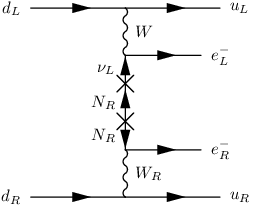

Figure 3: Feynman diagrams of double beta decay in the left-right symmetric model with final state electrons of different helicity: (a) the -mechanism and (b) the -mechanism due to gauge boson mixing. - •
Fig. 2 is a diagram mediated by the triplet of . The amplitude is given by
(12) The diagram is suppressed with respect to the standard light neutrino exchange by at least a factor .
- •
- •
Finally, Fig. 3 is another diagram with mixed helicity, possible due to mixing, which is described by the parameter defined in Eq. (A-21). The amplitude is
(15) with particle physics parameter
(16) Note that in both the - and -diagrams there are light neutrinos exchanged (long-range diagrams), and the amplitude is proportional to the mixing matrix . One therefore needs both a non-zero and , which is illustrated by the Dirac and Majorana mass terms in the propagator. In this case lepton number violation is implicit: the mixing vanishes for infinite Majorana mass. Ref. [3] gives a detailed explanation of how a complicated cancellation of different nuclear physics amplitudes leads to a limit on the -diagram that is much stronger than the one on the -diagram.
Having written down all interesting diagrams, it is instructive to
discuss their expected relative magnitudes. For this naive exercise,
let us denote the masses of all particles belonging to the
right-handed sector (, and ) as . The matrices
and describing left-right mixing can be written as , where
is about GeV, corresponding to the weak scale, or the mass of
the . The gauge boson mixing angle is at most of order
, and can be much smaller22
2
See Eq. (A-23) and the comments just below it.. The mixed - and -diagrams in
Fig. 3 are of order , whereas
the purely right-handed short-range diagrams in
Figs. 1 (heavy neutrino exchange and right-handed
currents) and 2 ( triplet exchange and
right-handed currents) are of order . Therefore, with
being of order TeV, the mixed diagrams are expected to dominate
by a factor . In the same sense, the amplitudes
of the mixed diagrams are also larger than the one for heavy neutrino
exchange with left-handed currents (which is proportional to
). Leaving these estimates aside, we continue with a purely
phenomenological analysis of the different diagrams at a linear collider.
For this exercise, let us use crossing symmetry to translate the -diagrams from Figs. 1–3 into linear collider cross sections of the form (Fig. 4). In each case the two gauge bosons can either have the same polarization ( or ), in which case the process can be mediated by either Majorana neutrinos or Higgs triplets, or opposite polarizations (), only possible with the exchange of Majorana neutrinos plus non-zero left-right mixing. Since the limits on are 2.5 TeV [38, 39], diagrams with two are obviously disfavoured. In what regards diagrams with two , both the light and the heavy neutrino exchange can be shown to be suppressed and unobservable, see Ref. [18] for a recent reanalysis. The cross section corresponding to left-handed triplet exchange [Fig. 2] is proportional to (see Eq. (A-12) and Ref. [35]), so that it is suppressed by light neutrino mass. We are left with diagrams with only one , i.e. the mixed diagrams from Fig. 3. Noting that the limit on the -diagram is less stringent by almost two orders of magnitude with respect to the one for [compare Eqs. (14) and (16)], we are led to the conclusion that the -diagram is the most promising channel to study. Fig. 4 shows the relevant Feynman diagram; its cross section will be evaluated in what follows. Let us note here that the SuperNEMO experiment has the possibility to disentangle the -diagram from the standard one, because it can probe the angular and energy correlation of the two emitted electrons in [36]. The mechanism is therefore testable in a variety of ways.


3 Cross section of
3.1 Cross section
The two possible channels for the process are shown in Fig. 4. Here and are the momenta of the particles and , the Lorentz indices of the polarization vectors. The matrix element is
| (17) |
where the subscript denotes the - or -channel process. In order to evaluate the differential cross section
| (18) |
where , we need
| (19) |
The result is (neglecting )
| (20) | ||||
The interference term vanishes, since the final state particles are distinguishable. Fig. 5 shows the differential cross section as a function of , for TeV and TeV, normalized with respect to each other (the cross section for TeV is actually a factor of two smaller). is practically flat, and approaches a straight line as increases.

It is interesting to study the high energy behaviour of the total cross section in the case of light neutrino exchange. In the limit that , the cross section becomes
| (21) |
where the upper bound on is given in Eq. (14) and we have neglected the mass of the light neutrinos in the propagator. The apparent violation of unitarity can be explained by taking the full theory into account, in which case the cross section will vanish when and unitarity is restored (see Appendix B for details).
There is also another diagram analogous to Fig. 4, with heavy neutrinos exchanged. The structure of the matrix elements is the same, we need only to interchange , and , where is the mass of the heavy neutrinos and and are 33 mixing matrices defined in Eq. (A-15). In this case the rate for double beta decay will be suppressed with respect to the case of light neutrino exchange in the -diagram.
To calculate the total cross section the limits from experiments as well as the allowed region for must be taken into account. Fig. 6 shows the cross section for as a function of for TeV, assuming only light neutrinos are exchanged and with three different limits for : the solid (blue) line corresponds to the present upper limit [Eq. (14)] given by experiments, the dashed (green) uses a limit improved by a factor of and the dotted (red) line is for a limit improved by a factor of 2. Note that a factor of improvement in corresponds to a factor of improvement in life-time. We also indicate the cross section that would give five events at an integrated luminosity of 3000 [40], corresponding to a few years of running. It is evident that for , enough events are possible in case is observed soon, and caused by the -diagram. Note that since there is no Standard Model background to the process, a small rate is tolerable.
In the next subsection we will show that polarization of the electron beams could be used to enhance the cross section by up to a factor of two. Finally, we should note that in neutrinoless double beta decay different contributions could interfere destructively. In this case the bound on would be relaxed and a larger cross section is possible.

3.2 Polarized beams
Future linear colliders have the possibility to polarize their beams. In order to quantify the effects on our process, we define the polarization for an electron beam as follows:
| (22) |
where and stand for the number of electrons having right- and left-handed helicity in the electron beam 1 or 2, respectively. If beam 1 is fully left-handed, , whereas for a fully right-handed beam, .
| beam polarization | ||
|---|---|---|
| 1 | 2 | |
| 0% | 0% | 1 |
| 90% RH | 0% | |
| 50% LH | 50% LH | |
| 50% LH | 50% RH | |
| 80% LH | 50% RH | |
| 90% LH | 90% RH | |
| 90% LH | 80% RH | |
| 100% LH | 100% RH | |
When the electron beam 1 has a polarization of and the electron beam 2 has a polarization of , the total cross section of a process is calculated as
| (23) |
where stands for the cross section of the process when both electron beams are 100% polarized, one left-handed and the other right-handed; , and are defined in a similar way. In our case for the -diagram , and () is the cross section that would arise from the -channel (-channel) diagram only. Furthermore, . Thus, equation (23) simply becomes
| (24) |
Table 1 gives numerical examples. We have defined the ratio between the cross section of polarized and unpolarized beams:
| (25) |
Obviously, is the total cross section calculated before. We see that the event numbers can in principle be doubled. Furthermore, polarization could be used as an additional method to distinguish different mechanisms for processes of the form . For instance, the process jets [19] mediated by -parity violating supersymmetry, involves slepton exchange, which couple mainly to left-handed electrons.
4 Conclusion
We have considered in this paper the process as a clean check of the so-called -diagram as the leading contribution to neutrinoless double beta decay. We argued that among the many possible diagrams for that are possible in left-right symmetric theories, it is the most promising one at a linear collider. Indeed, it may be possible to observe the process at a linear collider with center-of-mass energy of 3 TeV. It is however necessary that both the mass of the and the life-time of are close to their current experimental limits. We have also considered beam polarization effects and the high energy behaviour of the total cross section, as well as the individual amplitudes.
Acknowledgements
We thank Steve Kom for helpful comments. This work was supported by the ERC under the Starting Grant MANITOP (JB and WR) as well as by a CSIC JAE predoctoral fellowship, by the Spanish MEC under grants FPA2008-00319/FPA, FPA2011-22975 and MULTI-DARK CSD2009-00064 (Consolider-Ingenio 2010 Programme), by Prometeo/2009/091 (Generalitat Valenciana) and by the EU ITN UNILHC PITN-GA-2009-237920 (LD). LD would like to thank the Max-Planck-Institut für Kernphysik in Heidelberg for kind hospitality.
Appendix
Appendix A Details of the left-right symmetric model
In the left-right symmetric model [41, 42, 43, 44, 45], the Standard Model is extended to include the gauge group (with gauge coupling ), and right-handed fermions are grouped into doublets under this group. Thus we have the following fermion particle content under :
| (A-1) | |||||
| (A-2) |
with the electric charge given by and . The subscripts and are associated with the projection . In order to break the gauge symmetry and allow Majorana mass terms for neutrinos one introduces the Higgs triplets
| (A-3) |
with and ; the electroweak symmetry is broken by the bi-doublet scalar
| (A-4) |
The relevant Lagrangian in the lepton sector is
| (A-5) |
where ; and are matrices of Yukawa couplings and charge conjugation is defined as
| (A-6) |
If one assumes a discrete LR symmetry in addition to the additional gauge symmetry, the gauge couplings become equal () and one obtains relations between the Yukawa coupling matrices in the model. With a discrete parity symmetry it follows that , , ; with a charge conjugation symmetry , , .
Making use of the gauge symmetry to eliminate complex phases, the most general vacuum is
| (A-7) |
After spontaneous symmetry breaking, the mass term for the charged leptons is
| (A-8) |
where the mass matrix
| (A-9) |
can be diagonalized by the bi-unitary transformation
| (A-10) |
In the neutrino sector we have a type I + II seesaw scenario,
| (A-11) |
with
| (A-12) |
Assuming that , the light neutrino mass matrix can be written in terms of the model parameters as
| (A-13) |
where
| (A-14) |
The symmetric neutrino mass matrix in Eq. (A-11) is diagonalized by the unitary matrix [46, 47, 48]
| (A-15) |
to , where the matrices and are defined by
| (A-16) |
The neutrino mass eigenstates are defined by
| (A-17) | ||||
| (A-18) |
Note that the unitarity of leads to the useful relations
| (A-19) |
with the unitary matrices and defined in Eq. (A-15).
The leptonic charged current interaction in the flavour basis is
| (A-20) |
where
| (A-21) |
characterizes the mixing between left- and right-handed gauge bosons, with . With negligible mixing the gauge boson masses become
| (A-22) |
and assuming that33 3 This is justified if one assumes no cancellations in generating quark masses [49]. , it follows that
| (A-23) |
so that the mixing angle is at most44 4 Although the experimental limit is [50], for one has [51]; supernova bounds for right-handed neutrinos lighter than 1 MeV are even more stringent () [52, 51, 53]. the square of the ratio of left and right scales . The charged current then becomes
| (A-24) |
Here and are mixing matrices
| (A-25) |
connecting the three charged lepton mass eigenstates to the six neutrino mass eigenstates , (), with [using Eq. (A-19)] and .
Appendix B High energy behaviour of
Naively, the high-energy limit of the cross section is obtained by neglecting the neutrino mass in the propagator [see Eq. (20)], i.e.
| (A-27) |
which does not seem to vanish. However, one needs to consider the full theory. In calculating the cross section one combines two terms from the Lagrangian in Eq. (A-24):
| (A-28) |
The identity allows one to contract to a propagator, so that in the high energy limit the amplitude is proportional to
| (A-29) |
instead of as in the naive case. As shown in the previous subsection, , which means that the cross section vanishes in the high energy limit and unitarity is ensured.
Appendix C Helicity amplitudes for
It is an illustrative exercise to evaluate the helicity amplitudes of the process , with the helicity of the electrons and the polarization of the -bosons fixed. Denoting electron (-boson) momenta with (), (), the process is
| (A-30) |
where and . Without loss of generality, one can choose and to be in the -directions, and assume that the final state particles propagate in the – plane. The momenta are then given by
| (A-31) |
where and
| (A-32) |
The gauge boson polarization vectors can be defined by
| (A-33) | ||||
| (A-34) |
The helicity amplitudes are calculated from
| (A-35) |
resulting in
| (A-36) | ||||
| (A-37) | ||||
| (A-38) | ||||
| (A-39) | ||||
| (A-40) | ||||
| (A-41) |
where and , and when . The amplitude vanishes whenever , or in other words, when the two electrons have the same spin (note that one electron is described by a spinor in Eq. (A-35), which means that its actual helicity is the opposite of the spinor’s helicity). The amplitude is only non-zero when the electrons have opposite spin (); squaring and summing over boson polarizations gives the polarized cross sections and in Eq. (23), which correspond to the - and -channels respectively.
It is interesting to study the high energy behaviour of these helicity amplitudes. Explicitly, in the limit and neglecting neutrino mass one gets
| (A-42) | ||||
The amplitudes that contain at least one longitudinally polarized -boson () are divergent, whereas those with only transverse polarizations () are finite. Summing over fermion spins and boson polarizations gives the result in Eq. (21), and proper consideration of the full theory will lead to a well-behaved total amplitude, in analogy to Appendix B.
References
- [1] F. T. I. Avignone, S. R. Elliott, and J. Engel, Rev.Mod.Phys. 80, 481 (2008), 0708.1033.
- [2] J. Gomez-Cadenas et al., Riv.Nuovo Cim. 35, 29 (2012), 1109.5515.
- [3] J. Vergados, Phys.Rept. 361, 1 (2002), hep-ph/0209347.
- [4] W. Rodejohann, Int. J. Mod. Phys. E20, 1833 (2011), 1106.1334.
- [5] T. G. Rizzo, Phys.Lett. B116, 23 (1982).
- [6] D. London, G. Belanger, and J. Ng, Phys.Lett. B188, 155 (1987).
- [7] K. Huitu, J. Maalampi, and M. Raidal, Nucl.Phys. B420, 449 (1994), hep-ph/9312235.
- [8] T. G. Rizzo, Phys.Rev. D50, 5602 (1994), hep-ph/9404225.
- [9] P. Helde, K. Huitu, J. Maalampi, and M. Raidal, Nucl.Phys. B437, 305 (1995), hep-ph/9409320.
- [10] J. Gluza and M. Zralek, Phys.Rev. D52, 6238 (1995), hep-ph/9502284.
- [11] G. Belanger, F. Boudjema, D. London, and H. Nadeau, Phys. Rev. D53, 6292 (1996), hep-ph/9508317.
- [12] B. Ananthanarayan and P. Minkowski, Phys.Lett. B373, 130 (1996), hep-ph/9512271.
- [13] T. G. Rizzo, Int.J.Mod.Phys. A11, 1613 (1996), hep-ph/9510349.
- [14] C. A. Heusch and P. Minkowski, (1996), hep-ph/9611353.
- [15] J. Gluza, Phys.Lett. B403, 304 (1997), hep-ph/9704202.
- [16] P. Duka, J. Gluza, and M. Zralek, Phys.Rev. D58, 053009 (1998), hep-ph/9804372.
- [17] J. Maalampi and N. Romanenko, Phys.Rev. D60, 055002 (1999), hep-ph/9810528.
- [18] W. Rodejohann, Phys. Rev. D81, 114001 (2010), 1005.2854.
- [19] C. Kom and W. Rodejohann, Phys.Rev. D85, 015013 (2012), 1110.3220.
- [20] W.-Y. Keung and G. Senjanovic, Phys.Rev.Lett. 50, 1427 (1983).
- [21] A. Ferrari et al., Phys.Rev. D62, 013001 (2000).
- [22] V. Tello, M. Nemevsek, F. Nesti, G. Senjanovic, and F. Vissani, Phys.Rev.Lett. 106, 151801 (2011), 1011.3522.
- [23] M. Nemevsek, F. Nesti, G. Senjanovic, and V. Tello, (2011), 1112.3061.
- [24] B. Allanach, C. Kom, and H. Pas, Phys.Rev.Lett. 103, 091801 (2009), 0902.4697.
- [25] B. Allanach, C. Kom, and H. Pas, JHEP 0910, 026 (2009), 0903.0347.
- [26] CMS Collaboration, CMS-PAS-EXO-11-002 (2011).
- [27] ATLAS Collaboration, G. Aad et al., Phys.Lett. B705, 28 (2011), 1108.1316.
- [28] ATLAS Collaboration, G. Aad et al., (2012), 1203.5420.
- [29] F. J. Almeida et al., Eur.Phys.J. C38, 115 (2004), hep-ph/0405020.
- [30] P. Langacker, Rev.Mod.Phys. 81, 1199 (2009), 0801.1345.
- [31] K. Huitu, J. Maalampi, A. Pietila, and M. Raidal, Nucl.Phys. B487, 27 (1997), hep-ph/9606311.
- [32] A. Melfo, M. Nemevsek, F. Nesti, G. Senjanovic, and Y. Zhang, Phys.Rev. D85, 055018 (2012), 1108.4416.
- [33] ATLAS Collaboration, G. Aad et al., Phys.Rev. D88, 032004 (2012), 1201.1091.
- [34] G. Barenboim, K. Huitu, J. Maalampi, and M. Raidal, Phys.Lett. B394, 132 (1997), hep-ph/9611362.
- [35] W. Rodejohann and H. Zhang, Phys.Rev. D83, 073005 (2011), 1011.3606.
- [36] SuperNEMO Collaboration, R. Arnold et al., Eur.Phys.J. C70, 927 (2010), 1005.1241.
- [37] M. Hirsch, H. V. Klapdor-Kleingrothaus, and O. Panella, Phys. Lett. B374, 7 (1996), hep-ph/9602306.
- [38] A. Maiezza, M. Nemevsek, F. Nesti, and G. Senjanovic, Phys.Rev. D82, 055022 (2010), 1005.5160.
- [39] D. Guadagnoli and R. N. Mohapatra, Phys.Lett. B694, 386 (2011), 1008.1074.
- [40] E. Adli et al., http://project-clic-cdr.web.cern.ch/project-CLIC-CDR/.
- [41] R. Mohapatra and J. C. Pati, Phys.Rev. D11, 2558 (1975).
- [42] J. C. Pati and A. Salam, Phys.Rev. D10, 275 (1974).
- [43] G. Senjanovic and R. N. Mohapatra, Phys.Rev. D12, 1502 (1975).
- [44] R. N. Mohapatra and G. Senjanovic, Phys.Rev. D23, 165 (1981).
- [45] N. Deshpande, J. Gunion, B. Kayser, and F. I. Olness, Phys.Rev. D44, 837 (1991).
- [46] J. Schechter and J. W. F. Valle, Phys. Rev. D25, 774 (1982).
- [47] W. Grimus and L. Lavoura, JHEP 0011, 042 (2000), hep-ph/0008179.
- [48] H. Hettmansperger, M. Lindner, and W. Rodejohann, JHEP 1104, 123 (2011), 1102.3432.
- [49] Y. Zhang, H. An, X. Ji, and R. N. Mohapatra, Nucl.Phys. B802, 247 (2008), 0712.4218.
- [50] Particle Data Group, K. Nakamura et al., J.Phys.G G37, 075021 (2010).
- [51] P. Langacker and S. U. Sankar, Phys.Rev. D40, 1569 (1989).
- [52] G. Raffelt and D. Seckel, Phys.Rev.Lett. 60, 1793 (1988).
- [53] R. Barbieri and R. N. Mohapatra, Phys.Rev. D39, 1229 (1989).