跳到论文正文
W Papers独立论文阅读器 arXiv:1203.3135 论文正文 计算阅读时间 · 0%
引用这篇论文根据当前论文元数据生成,正式投稿前建议核对。


License: arXiv.org perpetual non-exclusive license
arXiv:1203.3135v1 [math.ST] 14 Mar 2012

Adaptive wavelet estimation of a compound Poisson process

Céline Duval Note: GIS-CREST and CNRS-UMR 8050, 3, avenue Pierre Larousse, 92245 Malakoff Cedex, France.
Abstract

We study the nonparametric estimation of the jump density of a compound Poisson process from the discrete observation of one trajectory over [0,T][0,T]. We consider the microscopic regime when the sampling rate Δ=ΔT→0\Delta=\Delta_{T}\rightarrow 0 as T→∞T\rightarrow\infty. We propose an adaptive wavelet threshold density estimator and study its performance for the LpL_{p} loss, p≥1p\geq 1, over Besov spaces. The main novelty is that we achieve minimax rates of convergence for sampling rates ΔT\Delta_{T} that vanish with TT at arbitrary polynomial rates. More precicely, our estimator attains minimax rates of convergence provided there exists a constant K≥1K\geq 1 such that the sampling rate ΔT\Delta_{T} satisfies T​ΔT2​K+2≤1.T\Delta_{T}^{2K+2}\leq 1. If this condition cannot be satisfied we still provide an upper bound for our estimator. The estimating procedure is based on the inversion of the compounding operator in the same spirit as Buchmann and Grübel (2003).

AMS 2000 subject classifications: 62G99, 62M99, 60G50.
Keywords: Compound Poisson process, Discretely observed random process, Decompounding, Wavelet density estimation.

1 Introduction

1.1 Statistical setting

Let RR be a standard homogeneous Poisson process with intensity ϑ\vartheta in (0,∞)(0,\infty), we define the compound Poisson process XX as

Xt\displaystyle X_{t} =∑i=1Rtξi,t≥0\displaystyle=\sum_{i=1}^{R_{t}}\xi_{i},\ \ \ \ \ t\geq 0

where the (ξi)\big(\xi_{i}\big) are independent and identically distributed random variables and independent of the Poisson process RR.

Assume that we have discrete observations of the process XX over [0,T][0,T] at times i​Δi\Delta for some Δ>0\Delta>0

(XΔ,…,X⌊T​Δ−1⌋​Δ).\big(X_{\Delta},\ldots,X_{\lfloor T\Delta^{-1}\rfloor\Delta}\big). (1)

We focus on the microscopic regime, namely

Δ=ΔT→0 as ​T→∞\Delta=\Delta_{T}\rightarrow 0\ \ \ \ \ \mbox{ as }\ T\rightarrow\infty

and work under the following assumption.

Assumption 1.

The law of the ξi\xi_{i} has density ff which is absolutely continuous with respect to the Lebesgue measure.

We denote by ℱ⁡(ℝ)\mathcal{F}(\mathbb{R}) the space of densities with respect to the Lebesgue measure supported by ℝ\mathbb{R}. We investigate the nonparametric estimation of the density ff on a compact interval 𝒟\mathcal{D} included in ℝ\mathbb{R} from the observations (1). To that end we use wavelet threshold density estimators and study their rate of convergence uniformly over Besov balls for the following loss function

(𝔼⁡[‖f^−f‖Lp​(𝒟)p])1/p,\displaystyle\big(\mathbb{E}\big[\|\widehat{f}-f\|_{L_{p}(\mathcal{D})}^{p}\big]\big)^{1/p}, (2)

where f^\widehat{f} is an estimator of ff, p≥1p\geq 1 and

‖f‖Lp​(𝒟)=(∫𝒟|f⁡(x)|p​𝑑x)1/p.\|f\|_{L_{p}(\mathcal{D})}=\Big(\int_{\mathcal{D}}|f(x)|^{p}dx\Big)^{1/p}.

We also denote by ‖f‖Lp​(ℝ)\|f\|_{L_{p}(\mathbb{R})} the usual LpL_{p} norm for p≥1p\geq 1

‖f‖Lp​(ℝ)=(∫ℝ|f⁡(x)|p​𝑑x)1/p.\|f\|_{L_{p}(\mathbb{R})}=\Big(\int_{\mathbb{R}}|f(x)|^{p}dx\Big)^{1/p}.

We do not assume the intensity ϑ\vartheta to be known: it is a nuisance parameter.

By Assumption 1, on the event {Xi​Δ−X(i−1)​Δ=0}\{X_{i\Delta}-X_{(i-1)\Delta}=0\} no jump occurred between (i−1)​Δ(i-1)\Delta and i​Δi\Delta and the increment Xi​Δ−X(i−1)​ΔX_{i\Delta}-X_{(i-1)\Delta} gives no information on ff. In the microscopic regime many increments are zero, therefore to estimate ff we focus on the nonzero increments and denote by NTN_{T} their number over [0,T][0,T]. In that statistical context different difficulties arise. First the sample size NTN_{T} is random. Second on the event {Xi​Δ−X(i−1)​Δ≠0}\{X_{i\Delta}-X_{(i-1)\Delta}\neq 0\}, the increment Xi​Δ−X(i−1)​ΔX_{i\Delta}-X_{(i-1)\Delta} is not necessarily a realisation of the density ff. Indeed even if Δ\Delta is small there is always a positive probability that more than one jump occurred between (i−1)​Δ(i-1)\Delta and i​Δi\Delta. Conditional on {Xi​Δ−X(i−1)​Δ≠0}\{X_{i\Delta}-X_{(i-1)\Delta}\neq 0\}, the law of Xi​Δ−X(i−1)​ΔX_{i\Delta}-X_{(i-1)\Delta} has density given by (see Proposition 1 in Section 2 below)

𝐏Δ​[f]​(x)=∑m=1∞ℙ⁡(RΔ=m|RΔ≠0)​f⋆m​(x), for ​x∈ℝ,\displaystyle\mathbf{P}_{\Delta}[f](x)=\sum_{m=1}^{\infty}\mathbb{P}\big(R_{\Delta}=m\big|R_{\Delta}\neq 0\big)f^{\star m}(x),\ \ \ \ \mbox{ for }x\in\mathbb{R}, (3)

where ⋆\star is the convolution product and f⋆m=f⋆…⋆ff^{\star m}=f\star\ldots\star f, mm times.

Adaptive estimators of the density ff in that statistical context already exists. Under the condition T​ΔT≤1T\Delta_{T}\leq 1 (or T​ΔT2≤1T\Delta_{T}^{2}\leq 1 if ff is smooth enough), they attain minimax rates of convergence over Sobolev spaces for the L2L_{2} loss (see Bec and Lacour [1], Comte and Genon-Catalot [4, 6] and Figueroa-López [10]). In this paper we try to answer the following questions.

  • i)

    Is it possible to construct an estimator of ff when ΔT\Delta_{T} decays slowly to 0, for instance when ΔT\Delta_{T} vanishes polynomially slowly with TT.

  • ii)

    Is it possible to construct adaptive wavelet estimators that attain, over Besov spaces for the LpL_{p} loss defined in (2), the classical minimax rates of convergence of the experiment where we observe TT independent realisations of ff.

Without loss of generality, assuming TT is an integer if we observe TT independent realisations of a density ff of regularity ss measured with the LπL_{\pi} norm, π>0\pi>0, it is possible to achieve the minimax rates of convergence for the LpL_{p} loss –up to constants and logarithmic factors– which is of the form

T−α⁡(s,π,p)T^{-\alpha(s,\pi,p)}

where α⁡(s,π,p)≤1/2\alpha(s,\pi,p)\leq 1/2 (see for instance Donoho et al. [7] and (16) hereafter). When the process XX is continuously observed over [0,T][0,T], we have RTR_{T} independent and identically distributed realisations of ff. Moreover for TT large enough, RTR_{T} is of the order of TT. That is why we want compare the performance of estimators of ff in the regime ΔT→0\Delta_{T}\rightarrow 0 with the classical minimax rate we would have if XX were continuously observed.

1.2 Our Results

We build our estimator of ff using equation (3) and proceed in two steps. The first step is the computation of the inverse of the operator f→𝐏Δ​[f]f\rightarrow\mathbf{P}_{\Delta}[f]. The inverse takes the form

𝐏Δ−1​[ν]=∑m≥1∞am​(ϑ,ΔT)​ν⋆m,ν∈ℱ⁡(ℝ)\mathbf{P}_{\Delta}^{-1}[\nu]=\sum_{m\geq 1}^{\infty}a_{m}(\vartheta,\Delta_{T})\nu^{\star m},\ \ \ \ \nu\in\mathcal{F}(\mathbb{R})

where the (am​(ϑ,ΔT))\big(a_{m}(\vartheta,\Delta_{T})\big) are explicit (see Proposition 1 below). They depend on the intensity ϑ\vartheta and can be estimated. We take advantage of

f≈𝐋Δ,K​[𝐏Δ​[f]],\displaystyle f\approx\mathbf{L}_{\Delta,K}\big[\mathbf{P}_{\Delta}[f]\big], (4)

where 𝐋Δ,K\mathbf{L}_{\Delta,K} is the Taylor expansion of order KK in Δ\Delta of 𝐏Δ−1\mathbf{P}_{\Delta}^{-1}. It depends only on (𝐏Δ​[f]⋆m,m=1,…,K+1)\big({\mathbf{P}_{\Delta}}[f]^{\star m},m=1,\ldots,K+1\big). That step can be referred as decoumpounding as introduced in Buchmann et al. [2].

The second step consists in estimating the densities 𝐏Δ​[f]⋆m\mathbf{P}_{\Delta}[f]^{\star m}, for m=1,…,K+1m=1,\ldots,K+1. For that we use the NTN_{T} nonzero increments which are independent and with density 𝐏Δ​[f]\mathbf{P}_{\Delta}[f]. The difficulty here is that NTN_{T} is random. In Theorem 1 we show that conditional on NTN_{T} wavelet threshold estimators of 𝐏Δ​[f]⋆m\mathbf{P}_{\Delta}[f]^{\star m} attain a rate of convergence –up to logarithmic factors– in NT−α⁡(s,π,p)N_{T}^{-\alpha(s,\pi,p)}. For TT large enough we prove (see Proposition 2 in Section 5) that NTN_{T} concentrates around a deterministic value of the order of TT, giving an unconditional rate of convergence in T−α⁡(s,π,p)T^{-\alpha(s,\pi,p)}. We inject those estimators into 𝐋Δ,K\mathbf{L}_{\Delta,K}, defined in (4), and obtain an estimator of ff that we call estimator corrected at order KK.

The study of the rate of convergence of the estimator corrected at order KK requires to control two distinct error terms. A deterministic one due the first step which is the error made when approximating ff by 𝐋Δ,K​[𝐏Δ​[f]]\mathbf{L}_{\Delta,K}\big[\mathbf{P}_{\Delta}[f]\big] in (4). And a statistical one due to the replacement of the 𝐏Δ​[f]⋆m{\mathbf{P}_{\Delta}}[f]^{\star m} by estimators in the second step. The deterministic error decreases when KK increases, then the idea is to choose KK sufficiently large for the deterministic error term to be negligible in front of the statistical one. We give in Theorem 1 an upper bound for the rate of convergence of the estimator corrected at order KK which is in –up to constants and logarithmic factors–

max⁡{T−α⁡(s,π,p),ΔTK+1}.\max\{T^{-\alpha(s,\pi,p)},\Delta_{T}^{K+1}\}.

It decreases with KK and if there exists K0K_{0} such that

T​ΔT2​K0+2≤1,\displaystyle T\Delta_{T}^{2K_{0}+2}\leq 1, (5)

since α⁡(s,π,p)≤1/2\alpha(s,\pi,p)\leq 1/2 the estimator corrected at order K0K_{0} attains the minimax rates of convergence. It follows that for every ΔT\Delta_{T} polynomially decreasing with TT, it is possible to exhibit K0K_{0} such that (5) is valid and the estimator corrected at order K0K_{0} provides a positive answer to i) and ii). If no KK enables to verify condition (5), Theorem 1 provides an upper bound for the rate of convergence of the estimator corrected at order KK, in that case the estimator still provide a positive answer to i).

In the case of a compound Poisson processes, the results of the present paper generalise to some extend those of Bec and Lacour [1], Comte and Genon-Catalot [4, 6] and Figueroa-López [10]. This is discussed in further details in Section 4. In Section 2 we give the main results of the paper. We properly define wavelet functions and Besov spaces used for the estimation before having a complete construction of the estimator corrected at order KK. Then we give an upper bound for its rate of convergence for the LpL_{p} loss defined in (2), p≥1p\geq 1, uniformly over Besov balls. A numerical example illustrates the behavior of the estimator corrected at order KK in Section 3. Finally Section 5 is dedicated to the proofs.

The model of this paper is central in many application fields e.g. statistical physics (see Moharir [17]), biology (see Huelsenbeck et al. [13]), financial series or mathematical insurance (see Scalas [19]). It is well adapted to study phenomena where random independent events occur at random times. For instance, in insurance failure theory these events can model the claims that insurance companies have to pay to the subscribers. The insurer’s surplus at a given time tt can be modeled by the following process

K⁡(t)=K0+k​t−Xt,\displaystyle K(t)=K_{0}+kt-X_{t},

where K0K_{0} is the capital of the company at time 0, the second term is a deterministic trend corresponding to the average income received from the subscribers and XX is a compound Poisson process modeling the insurance claims occurring at random times with random amount of money at stake. It is the Cramér-Lundberg model; see Embrechts et al. [8] or Scalas [19]. Compound Poisson processes can also model the changes of an asset price in finance; see Masoliver et al. [15].

2 Main results

2.1 Besov spaces and wavelet thresholding

To estimate the densities (𝐏Δ​[f]⋆m,m=1,…,K+1)\big({\mathbf{P}_{\Delta}}[f]^{\star m},m=1,\ldots,K+1\big) we use wavelet threshold density estimators and study their performance uniformly over Besov balls. In this paragraph we reproduce some classical results on Besov spaces, wavelet bases and wavelet threshold estimators (see Cohen [3], Donoho et al. [7] or Kerkyacharian and Picard [14]) that we use in the next sections.

Wavelets and Besov spaces

We describe the smoothness of a function with Besov spaces on 𝒟\mathcal{D}. We recall here some well documented results on Besov spaces and their connection to wavelet bases (see Cohen [3], Donoho et al. [7] or Kerkyacharian and Picard [14]). Let (ψλ)λ\big(\psi_{\lambda}\big)_{\lambda} be a regular wavelet basis adapted to the domain 𝒟\mathcal{D}. The multi-index λ\lambda concatenates the spatial index and the resolution level j=|λ|j=|\lambda|. Set Λj:={λ,|λ|=j}\Lambda_{j}:=\{\lambda,|\lambda|=j\} and Λ=∪j≥−1Λj\Lambda=\cup_{j\geq-1}\Lambda_{j}, for ff in Lp​(ℝ)L_{p}(\mathbb{R}) we have

f\displaystyle f =∑j≥−1∑λ∈Λj⟨f,ψλ⟩​ψλ,\displaystyle=\sum_{j\geq-1}\sum_{\lambda\in\Lambda_{j}}\langle f,\psi_{\lambda}\rangle\psi_{\lambda}, (6)

where j=−1j=-1 incorporates the low frequency part of the decomposition and ⟨.,⟩\langle.,\rangle denotes the usual L2L_{2} inner product. We define Besov spaces in term of wavelet coefficients, for s>0s>0 and π∈(0,∞]\pi\in(0,\infty] a function ff belongs to the Besov space ℬπ​∞s​(𝒟)\mathcal{B}^{s}_{{\pi}\infty}(\mathcal{D}) if the norm

‖f‖ℬπ​∞s​(𝒟)\displaystyle\|f\|_{\mathcal{B}^{s}_{{\pi}\infty}(\mathcal{D})} :=supj≥−1​2j⁡(s+1/2−1/π)​(∑λ∈Λj|⟨f,ψλ⟩|π)1/π\displaystyle:=\underset{j\geq-1}{\sup}2^{j(s+1/2-1/\pi)}\Big(\sum_{\lambda\in\Lambda_{j}}|\langle f,\psi_{\lambda}\rangle|^{\pi}\Big)^{1/\pi} (7)

is finite, with usual modifications if π=∞\pi=\infty.

We need additional properties on the wavelet basis (ψλ)λ\big(\psi_{\lambda}\big)_{\lambda}, which are listed in the following assumption.

Assumption 2.

For p≥1p\geq 1,

  • •

    We have for some ℭ≥1\mathfrak{C}\geq 1

    ℭ−1​2|λ|​(p/2−1)≤‖ψλ‖Lp​(𝒟)p≤ℭ​2|λ|​(p/2−1).\mathfrak{C}^{-1}2^{|\lambda|(p/2-1)}\leq\|\psi_{\lambda}\|_{L_{p}(\mathcal{D})}^{p}\leq\mathfrak{C}2^{|\lambda|(p/2-1)}.
  • •

    For some ℭ>0\mathfrak{C}>0, σ>0\sigma>0 and for all s≤σs\leq\sigma, J≥0J\geq 0, we have

    ‖f−∑j≤J∑λ∈Λj⟨f,ψλ⟩​ψλ‖Lp​(𝒟)≤ℭ​2−J​s​‖f‖ℬπ​∞s​(𝒟).\displaystyle\big\|f-\sum_{j\leq J}\sum_{\lambda\in\Lambda_{j}}\langle f,\psi_{\lambda}\rangle\psi_{\lambda}\big\|_{L_{p}(\mathcal{D})}\leq\mathfrak{C}2^{-Js}\|f\|_{\mathcal{B}^{s}_{{\pi}\infty}(\mathcal{D})}. (8)
  • •

    If p≥1p\geq 1, for some ℭ≥1\mathfrak{C}\geq 1 and for any sequence of coefficients (uλ)λ∈Λ\big(u_{\lambda}\big)_{\lambda\in\Lambda},

    ℭ−1​‖∑λ∈Λuλ​ψλ‖Lp​(𝒟)≤‖(∑λ∈Λ|uλ​ψλ|2)1/2‖Lp​(𝒟)≤ℭ​‖∑λ∈Λuλ​ψλ‖Lp​(𝒟).\displaystyle\mathfrak{C}^{-1}\Big\|\sum_{\lambda\in\Lambda}u_{\lambda}\psi_{\lambda}\Big\|_{L_{p}(\mathcal{D})}\leq\Big\|\Big(\sum_{\lambda\in\Lambda}|u_{\lambda}\psi_{\lambda}|^{2}\Big)^{1/2}\Big\|_{L_{p}(\mathcal{D})}\leq\mathfrak{C}\Big\|\sum_{\lambda\in\Lambda}u_{\lambda}\psi_{\lambda}\Big\|_{L_{p}(\mathcal{D})}. (9)
  • •

    For any subset Λ0⊂Λ\Lambda_{0}\subset\Lambda and for some ℭ≥1\mathfrak{C}\geq 1

    ℭ−1​∑λ∈Λ0‖ψλ‖Lp​(𝒟)p≤∫𝒟(∑λ∈Λ0|ψλ​(x)|2)p/2≤ℭ​∑λ∈Λ0‖ψλ‖Lp​(𝒟)p.\displaystyle\mathfrak{C}^{-1}\sum_{\lambda\in\Lambda_{0}}\|\psi_{\lambda}\|_{L_{p}(\mathcal{D})}^{p}\leq\int_{\mathcal{D}}\Big(\sum_{\lambda\in\Lambda_{0}}|\psi_{\lambda}(x)|^{2}\Big)^{p/2}\leq\mathfrak{C}\sum_{\lambda\in\Lambda_{0}}\|\psi_{\lambda}\|_{L_{p}(\mathcal{D})}^{p}. (10)

Property (8) ensures that definition (7) of Besov spaces matches the definition in terms of linear approximation. Property (9) ensures that (ψλ)λ\big(\psi_{\lambda}\big)_{\lambda} is an unconditional basis of LpL_{p} and (10) is a super-concentration inequality (see Kerkyacharian and Picard [14] p. 304 and p. 306).

Wavelet threshold estimator

Let (ϕ,ψ)(\phi,\psi) be a pair of scaling function and mother wavelet that generate a basis (ψλ)λ\big(\psi_{\lambda}\big)_{\lambda} satisfying Assumption 2 for some σ>0\sigma>0. We rewrite (6)

f\displaystyle f =∑k∈Λ0α0​k​ϕ0​k+∑j≥1∑k∈Λjβj​k​ψj​k,\displaystyle=\sum_{k\in\Lambda_{0}}\alpha_{0k}\phi_{0k}+\sum_{j\geq 1}\sum_{k\in\Lambda_{j}}\beta_{jk}\psi_{jk},

where ϕ0​k(∙)=ϕ(∙−k)\phi_{0k}(\bullet)=\phi(\bullet-k) and ψj​k(∙)=2j/2ψ(2j∙−k)\psi_{jk}(\bullet)=2^{j/2}\psi(2^{j}\bullet-k) and

α0​k\displaystyle\alpha_{0k} =∫ϕ0​k​(x)​f​(x)​𝑑x\displaystyle=\int\phi_{0k}(x)f(x)dx
βj​k\displaystyle\beta_{jk} =∫ψj​k​(x)​f​(x)​𝑑x.\displaystyle=\int\psi_{jk}(x)f(x)dx.

For every j≥0j\geq 0, the set Λj\Lambda_{j} has cardinality 2j2^{j} and incorporates boundary terms that we choose not to distinguish in the notation for simplicity. An estimator of a function ff is obtained when replacing the (α0​k)(\alpha_{0k}) and (βj​k)(\beta_{jk}) by estimated values. In the sequel we uses (γj​k)(\gamma_{jk}) to design either (α0​k)(\alpha_{0k}) or (βj​k)(\beta_{jk}) and (gj​k)(g_{jk}) for the wavelet functions (ϕ0​k)(\phi_{0k}) or (ψj​k)(\psi_{jk}).

We consider classical hard threshold estimators of the form

f^​(∙)\displaystyle\widehat{f}(\bullet) =∑k∈Λ0α0​k^ϕ0​k(∙)+∑j=1J∑k∈Λjβj​k^𝟙{|βj​k^|≥η}ψj​k(∙),\displaystyle=\sum_{k\in\Lambda_{0}}\widehat{\alpha_{0k}}\phi_{0k}(\bullet)+\sum_{j=1}^{J}\sum_{k\in\Lambda_{j}}\widehat{\beta_{jk}}\mathds{1}_{\big\{|\widehat{\beta_{jk}}|\geq\eta\big\}}\psi_{jk}(\bullet),

where α0​k^\widehat{\alpha_{0k}} and βj​k^\widehat{\beta_{jk}} are estimators of α0​k\alpha_{0k} and βj​k\beta_{jk}, JJ and η\eta are respectively the resolution level and the threshold, possibly depending on the data. Thus to construct f^\widehat{f} we have to specify estimators (γj​k^)(\widehat{\gamma_{jk}}) of the (γj​k)(\gamma_{jk}) and the coefficients JJ and η\eta.

2.2 Construction of the estimator

Assume that we have ⌊T​Δ−1⌋\lfloor T\Delta^{-1}\rfloor discrete data at times i​Δi\Delta for some Δ>0\Delta>0 of the process XX

(XΔ,…,X⌊T​Δ−1⌋​Δ).\big(X_{\Delta},\ldots,X_{\lfloor T\Delta^{-1}\rfloor\Delta}\big).

Introduce the increments

𝐃ΔXi=Xi​Δ−X(i−1)​Δ, for i=1,…,⌊TΔ−1⌋,\displaystyle\mathbf{D}^{\Delta}X_{i}=X_{i\Delta}-X_{(i-1)\Delta},\ \ \ \mbox{ for }i=1,\dots,\lfloor T\Delta^{-1}\rfloor,

where X0=0X_{0}=0. They are independent and identically distributed since XX is a compound Poisson process. Define

S1\displaystyle S_{1} =inf{j,𝐃Δ​Xj≠0}∧T\displaystyle=\inf\big\{j,\mathbf{D}^{\Delta}X_{j}\neq 0\big\}\wedge T
Si\displaystyle S_{i} =inf{j>Si−1,𝐃Δ​Xj≠0}∧Tfor ​i≥1,\displaystyle=\inf\big\{j>S_{i-1},\mathbf{D}^{\Delta}X_{j}\neq 0\big\}\wedge T\ \ \ \mbox{for }i\geq 1,

where SiS_{i} is the random index of the iith jump and

NT=∑i=1⌊T​Δ−1⌋𝟙{𝐃ΔXi≠0}N_{T}=\sum_{i=1}^{\lfloor T\Delta^{-1}\rfloor}\mathds{1}_{\{\mathbf{D}^{\Delta}X_{i}\neq 0\}}

the random number of nonzero increments observed over [0,T][0,T]. By Assumption 1, on the event {𝐃ΔXi=0},\{\mathbf{D}^{\Delta}X_{i}=0\}, no jump occurred between (i−1)​Δ(i-1)\Delta and i​Δi\Delta. In the microscopic regime when Δ=ΔT→0\Delta=\Delta_{T}\rightarrow 0 as TT goes to infinity many increments are null and convey no information on ff, hence for the estimation of ff we focus on the nonzero ones

(𝐃Δ​XS1,…,𝐃Δ​XSNT).\big(\mathbf{D}^{\Delta}X_{S_{1}},\ldots,\mathbf{D}^{\Delta}X_{S_{N_{T}}}\big).
Proposition 1.

The distribution of the increment 𝐃Δ​XS1\mathbf{D}^{\Delta}X_{S_{1}} has density with respect to the Lebesgue measure given by

𝐏Δ​[f]\displaystyle\mathbf{P}_{\Delta}[f] =∑m=1∞pm​(Δ)​f⋆m,\displaystyle=\sum_{m=1}^{\infty}p_{m}(\Delta)f^{\star m},

where

pm​(Δ)=ℙ⁡(RΔ=m|RΔ≠0)=1eϑ​Δ−1​(ϑ​Δ)mm!.p_{m}(\Delta)=\mathbb{P}\big(R_{\Delta}=m|R_{\Delta}\neq 0\big)=\frac{1}{e^{\vartheta\Delta}-1}\frac{\big(\vartheta\Delta\big)^{m}}{m!}.

Let Δ0\Delta_{0} be such that

∑m=2∞(ϑ​Δ0)m−2m!≤1.\sum_{m=2}^{\infty}\frac{\big(\vartheta\Delta_{0}\big)^{m-2}}{m!}\leq 1.

For Δ≤Δ0\Delta\leq\Delta_{0}, we have that

1−ϑ​Δ≤p1​(Δ)≤1.1-\vartheta\Delta\leq p_{1}(\Delta)\leq 1.

It is straightforward to verify that the nonlinear operator 𝐏Δ\mathbf{P}_{\Delta} is a mapping from ℱ⁡(ℝ)\mathcal{F}(\mathbb{R}) to itself. The observations (𝐃Δ​XSi)\big(\mathbf{D}^{\Delta}X_{S_{i}}\big) are realisations of the density 𝐏Δ​[f]\mathbf{P}_{\Delta}[f] and by Proposition 1 the weight p1​(Δ)→1p_{1}(\Delta)\rightarrow 1 in the limit Δ=ΔT→0\Delta=\Delta_{T}\rightarrow 0. It follows that for ΔT\Delta_{T} small enough most of the (𝐃Δ​XSi)\big(\mathbf{D}^{\Delta}X_{S_{i}}\big) have distribution ff. Then a naive method to estimate ff is to apply classical density estimators to the (𝐃Δ​XSi)\big(\mathbf{D}^{\Delta}X_{S_{i}}\big). That estimator requires a convergence condition on ΔT\Delta_{T} to achieve minimax rate of convergence (see Theorem 1). However we wish to construct an estimator that attains minimax rates of convergence with weaker conditions on ΔT\Delta_{T}.

We adopt the estimating strategy of section 1.2 and construct an approximation of ff.

Lemma 1.

The inverse 𝐏Δ−1\mathbf{P}_{\Delta}^{-1} of 𝐏Δ\mathbf{P}_{\Delta}, such that for all densities ff in ℱ⁡(ℝ)\mathcal{F}(\mathbb{R}) if 𝐏Δ​[f]=ν\mathbf{P}_{\Delta}[f]=\nu we have 𝐏Δ−1​[ν]=f\mathbf{P}_{\Delta}^{-1}[\nu]=f, is given by

𝐏Δ−1​[ν]=1ϑ​Δ​∑m=1∞(−1)m+1m​(eϑ​Δ−1)m​ν⋆m.\displaystyle\mathbf{P}_{\Delta}^{-1}[\nu]=\frac{1}{\vartheta\Delta}\sum_{m=1}^{\infty}\frac{(-1)^{m+1}}{m}(e^{\vartheta\Delta}-1)^{m}\nu^{\star m}.

To build the estimator corrected at order KK we use that 𝐏Δ−1\mathbf{P}_{\Delta}^{-1} is a power series whose coefficients are equivalent to increasing powers of Δ\Delta. Then 𝐋Δ,K\mathbf{L}_{\Delta,K} the Taylor expansion of order KK in Δ\Delta of 𝐏Δ−1\mathbf{P}_{\Delta}^{-1} is obtained by keeping the first K+1K+1 terms of the inverse

𝐋Δ,K​[ν]=1ϑ​Δ​∑m=1K+1(−1)m+1m​(eϑ​Δ−1)m​ν⋆m,ν∈ℱ⁡(ℝ).\displaystyle\mathbf{L}_{\Delta,K}[\nu]=\frac{1}{\vartheta\Delta}\sum_{m=1}^{K+1}\frac{(-1)^{m+1}}{m}(e^{\vartheta\Delta}-1)^{m}\nu^{\star m},\ \ \ \nu\in\mathcal{F}(\mathbb{R}). (11)

Next we construct wavelet threshold density estimators of the first K+1K+1 convolution powers of 𝐏Δ​[f]{\mathbf{P}_{\Delta}}[f] that will be plugged in (11). Define

γ^j​k(m)\displaystyle\widehat{\gamma}^{(m)}_{jk} =1NT,m​∑i=1NT,mgj​k​(𝐃mΔ​XSi)m≥1,\displaystyle=\frac{1}{N_{T,m}}\sum_{i=1}^{N_{T,m}}g_{jk}\Big(\mathbf{D}^{\Delta}_{m}X_{S_{i}}\Big)\ \ \ \ m\geq 1, (12)

where NT,m=⌊NT/m⌋≥1N_{T,m}=\big\lfloor N_{T}/m\big\rfloor\geq 1 for large enough TT and

𝐃mΔ​XSi=𝐃Δ​XSi+𝐃Δ​XSNT,m+i+⋯+𝐃Δ​XS(m−1)​NT,m+i.\mathbf{D}^{\Delta}_{m}X_{S_{i}}=\mathbf{D}^{\Delta}X_{S_{i}}+\mathbf{D}^{\Delta}X_{S_{N_{T,m}+i}}+\dots+\mathbf{D}^{\Delta}X_{S_{(m-1)N_{T,m}+i}}.

The (𝐃Δ​XSi)\big(\mathbf{D}^{\Delta}X_{S_{i}}\big) are independent and identically distributed with density 𝐏Δ​[f]\mathbf{P}_{\Delta}[f], thus the (𝐃mΔ​XSi)\big(\mathbf{D}^{\Delta}_{m}X_{S_{i}}\big) are independent and identically distributed with density 𝐏Δ​[f]⋆m\mathbf{P}_{\Delta}[f]^{\star m}. Let η>0\eta>0 and J∈ℕ∖{0},J\in\mathbb{N}\setminus\{0\}, define PΔ,m^\widehat{P_{\Delta,m}} the estimator of 𝐏Δ​[f]⋆m\mathbf{P}_{\Delta}[f]^{\star m} over 𝒟\mathcal{D}

PΔ,m^​(x)\displaystyle\widehat{P_{\Delta,m}}(x) =∑kα^0​k(m)ϕ0​k(x)+∑j=0J∑kβ^j​k(m)𝟙{|β^j​k(m)|≥η}ψj​k(x),x∈𝒟.\displaystyle=\sum_{k}\widehat{\alpha}_{0k}^{(m)}\phi_{0k}(x)+\sum_{j=0}^{J}\sum_{k}\widehat{\beta}_{jk}^{(m)}\mathds{1}_{\big\{|\widehat{\beta}_{jk}^{(m)}|\geq\eta\big\}}\psi_{jk}(x),\ \ \ x\in\mathcal{D}. (13)
Definition 1.

We define f~T,ΔK\widetilde{f}^{K}_{T,\Delta} the estimator corrected at order KK for KK in ℕ\mathbb{N} and xx in 𝒟\mathcal{D} as

f~T,ΔK​(x)\displaystyle\widetilde{f}^{K}_{T,\Delta}(x) =∑m=1K+1(−1)m+1m​(eϑ^T​Δ−1)mϑ^T​Δ​PΔ,m^​(x),\displaystyle=\sum_{m=1}^{K+1}\frac{(-1)^{m+1}}{m}\frac{\big(e^{\widehat{\vartheta}_{T}\Delta}-1\big)^{m}}{\widehat{\vartheta}_{T}\Delta}\widehat{P_{\Delta,m}}(x), (14)

where

ϑ^T\displaystyle\widehat{\vartheta}_{T} =−1Δ​log⁡(1−p^T)\displaystyle=-\frac{1}{\Delta}\log(1-\widehat{p}_{T}) (15)

and

p^T=NT⌊T​Δ−1⌋\widehat{p}_{T}=\frac{N_{T}}{\lfloor T\Delta^{-1}\rfloor}

is the empirical estimator of p⁡(Δ)=ℙ⁡(RΔ=0)=1−e−ϑ​Δ.p(\Delta)=\mathbb{P}(R_{\Delta}=0)=1-e^{-\vartheta{\Delta}}.

Lemma 1 justifies the form of the estimator corrected at order KK.

2.3 Convergence rates

We estimate densities ff which verify a smoothness property in term of Besov balls

ℱ⁡(s,π,𝔐)={f∈ℱ⁡(ℝ),‖f‖ℬπ​∞s​(𝒟)≤𝔐},\mathcal{F}(s,{\pi},\mathfrak{M})=\big\{f\in\mathcal{F}(\mathbb{R}),\|f\|_{\mathcal{B}^{s}_{{\pi}\infty}(\mathcal{D})}\leq\mathfrak{M}\big\},

where 𝔐\mathfrak{M} is a positive constant. We are interested in estimating ff on the compact interval 𝒟\mathcal{D}, that is why we only impose that its restriction to 𝒟\mathcal{D} belongs to a Besov ball.

Theorem 1.

We work under Assumptions 1 and 2. Let σ>s>1/π\sigma>s>1/\pi, p≥1∧πp\geq 1\wedge\pi and PΔT,m^\widehat{P_{\Delta_{T},m}} be the threshold wavelet estimator of 𝐏ΔT​[f]⋆m\mathbf{P}_{\Delta_{T}}[f]^{\star m} on 𝒟\mathcal{D} constructed from (ϕ,ψ)(\phi,\psi) and defined in (13). Take JJ such that

2J​NT−1​log⁡(NT1/2)≤1,2^{J}N_{T}^{-1}\log\big(N_{T}^{1/2}\big)\leq 1,

and

η=κNT−1/2log⁡(NT1/2),\eta=\kappa N_{T}^{-1/2}\sqrt{\log\big(N_{T}^{1/2}\big)},

for some κ>0\kappa>0. Let

α⁡(s,p,π)=min⁡{s2​s+1,s+1/p−1/π2​(s+1/2−1/π)}.\displaystyle\alpha(s,p,\pi)=\min\Big\{\frac{s}{2s+1},\frac{s+1/p-1/{\pi}}{2\big(s+1/2-1/{\pi}\big)}\Big\}. (16)
  1. 1)

    The estimator PΔT,m^\widehat{P_{\Delta_{T},m}} verifies for large enough TT and sufficiently large κ>0\kappa>0

    sup𝐏ΔT​[f]⋆m∈ℱ⁡(s,π,𝔐)​(𝔼⁡[‖PΔT,m^−𝐏ΔT​[f]⋆m‖Lp​(𝒟)p|NT])1/p\displaystyle\underset{\mathbf{P}_{\Delta_{T}}[f]^{\star m}\in\mathcal{F}(s,{\pi},\mathfrak{M})}{\sup}\big(\mathbb{E}\big[\big\|\widehat{P_{\Delta_{T},m}}-\mathbf{P}_{\Delta_{T}}[f]^{\star m}\big\|_{L_{p}(\mathcal{D})}^{p}\big|N_{T}\big]\big)^{1/p} ≤ℭ​NT−α⁡(s,p,π),\displaystyle\leq\mathfrak{C}N_{T}^{-{\alpha(s,p,\pi)}},

    up to logarithmic factors in TT and where ℭ\mathfrak{C} depends on s,π,p,𝔐,ϕ,ψs,\pi,p,\mathfrak{M},\phi,\psi.

  2. 2)

    The estimator corrected at order KK f~T,ΔTK\widetilde{f}^{K}_{T,\Delta_{T}} defined in (14) verifies for TT large enough and any positive constants 𝔗¯\underline{\mathfrak{T}} and 𝔗¯\overline{\mathfrak{T}}

    supϑ∈[𝔗¯,𝔗¯]​supf∈ℱ⁡(s,π,𝔐)​(𝔼⁡[‖f~T,ΔTK−f‖Lp​(𝒟)p])1/p\displaystyle\underset{\vartheta\in[\underline{\mathfrak{T}},\overline{\mathfrak{T}}]}{\sup}\underset{f\in\mathcal{F}(s,{\pi},\mathfrak{M})}{\sup}\big(\mathbb{E}\big[\big\|\widetilde{f}^{K}_{T,\Delta_{T}}-f\big\|_{L_{p}(\mathcal{D})}^{p}\big]\big)^{1/p} ≤ℭ​max⁡{T−α⁡(s,p,π),ΔTK+1},\displaystyle\leq\mathfrak{C}\max\big\{T^{-{\alpha(s,p,\pi)}},\Delta_{T}^{K+1}\big\},

    up to logarithmic factors in TT and where ℭ\mathfrak{C} depends on s,π,p,𝔐,ϕ,ψ,𝔗¯,s,\pi,p,\mathfrak{M},\phi,\psi,\underline{\mathfrak{T}}, 𝔗¯,K\overline{\mathfrak{T}},K.

The proof of Theorem 1 is postponed to Section 5. From a practical point of view when one computes the estimator f~T,ΔTK\widetilde{f}^{K}_{T,\Delta_{T}} from (1) the sample size is NTN_{T}, which is why in Theorem 1 we give the resolution level JJ and the threshold η\eta as functions of NTN_{T} instead of replacing NTN_{T} by its deterministic counterpart. Explicit bound for κ\kappa is given in Lemma 4 hereafter.

In practice the values TT and ΔT\Delta_{T} are imposed or chosen by the practitioner. Theorem 1 ensures that the estimator corrected at order KK attains the minimax rate T−α⁡(s,p,π)T^{-{\alpha(s,p,\pi)}} for the smallest KK such that

ΔT=O⁡(T−α⁡(s,p,π)K+1).\Delta_{T}=O\big(T^{-\frac{{\alpha(s,p,\pi)}}{K+1}}\big).

Since α⁡(s,p,π)≤1/2\alpha(s,p,\pi)\leq 1/2 it is sufficient to choose KK such that

T​ΔT2​K+2=O⁡(1).T\Delta_{T}^{2K+2}=O(1).

If ΔT\Delta_{T} decays as a power of TT i.e. if there exists δ>0\delta>0 such that for some ℭ>0\mathfrak{C}>0

ΔT≤ℭ​T−δ,\Delta_{T}\leq\mathfrak{C}T^{-\delta},

it is always possible to find a correction level KK satisfying the previous constraint. The case K=0K=0 corresponds to the uncorrected estimator; it is the naive estimator one would compute making the approximation f≈𝐏Δ​[f]f\approx\mathbf{P}_{\Delta}[f]. In that case we get a rate of convergence in

max⁡{T−α⁡(s,p,π),ΔT},\max\{T^{-{\alpha(s,p,\pi)}},\Delta_{T}\},

which attains the minimax rate if Tα⁡(s,p,π)​ΔT≤1T^{\alpha(s,p,\pi)}\Delta_{T}\leq 1. Since α⁡(s,π,p)≤1/2\alpha(s,\pi,p)\leq 1/2, it follows that the condition Tα⁡(s,p,π)​ΔT≤1T^{\alpha(s,p,\pi)}\Delta_{T}\leq 1 already improves on the condition T​ΔT2≤1T\Delta_{T}^{2}\leq 1 of Bec and Lacour [1], Comte and Genon-Catalot [4, 6] or Figueroa-López [10] (see Section 4 for comparison with other works).

3 A numerical example

We illustrate the behaviour of the estimator corrected at order KK when KK increases and compare its performance with an oracle: the wavelet estimator we would compute in the idealised framework where all the jumps are observed

f^O​r​a​c​l​e(x)=∑kα^0​kO​r​a​c​l​eϕ0​k(x)+∑j=0J∑kβ^j​kO​r​a​c​l​e𝟙{|β^j​kO​r​a​c​l​e|≥η}ψj​k(x),\displaystyle\widehat{f}^{Oracle}(x)=\sum_{k}\widehat{\alpha}_{0k}^{Oracle}\phi_{0k}(x)+\sum_{j=0}^{J}\sum_{k}\widehat{\beta}_{jk}^{Oracle}\mathds{1}_{\big\{|\widehat{\beta}_{jk}^{Oracle}|\geq\eta\big\}}\psi_{jk}(x),

where

α^0​kO​r​a​c​l​e=1RT​∑i=1RTϕ0​k​(ξi)andβ^j​kO​r​a​c​l​e=1RT​∑i=1RTϕ0​k​(ξi),\widehat{\alpha}_{0k}^{Oracle}=\frac{1}{R_{T}}\sum_{i=1}^{R_{T}}\phi_{0k}(\xi_{i})\ \ \ \mbox{and}\ \ \ \widehat{\beta}_{jk}^{Oracle}=\frac{1}{R_{T}}\sum_{i=1}^{R_{T}}\phi_{0k}(\xi_{i}),

RTR_{T} being the value of the Poisson process RR at time TT and (ξi)(\xi_{i}) the jumps. The parameters JJ and η\eta as well as the wavelet bases (ϕ,ψ)(\phi,\psi) are the same as those used to compute the estimator corrected at order KK. We consider a compound Poisson process of intensity ϑ=1\vartheta=1 on [0,T][0,T] and of compound law

f⁡(x)=(1−a)​f1​(x)+a​f2​(x)\displaystyle f(x)=(1-a)f_{1}(x)+af_{2}(x)

where f1f_{1} is the density of a Gaussian 𝒩⁡(0,1)\mathcal{N}(0,1) and f2f_{2} of a Laplace with location parameter 1 and scale parameter 0.1, we take a=0.05a=0.05.

Refer to caption
Figure 1: Density f:f: f⁡(x)=0.95​f1​(x)+0.05​f2​(x)f(x)=0.95f_{1}(x)+0.05f_{2}(x) x∈[−6,6]x\in[-6,6].

We estimate the mixture ff (see Figure 1) on 𝒟=[−6,6]\mathcal{D}=[-6,6] with the estimator corrected at order KK for different values of KK and study the results with the L2L_{2} error. We also compare them with the oracle f^O​r​a​c​l​e\widehat{f}^{Oracle}. Wavelet estimators are based on the evaluation of the first wavelet coefficients, to perform those we use Symlets 4 wavelet functions and a resolution level J=10J=10. Moreover we transform the data in an equispaced signal on a grid of length 2L2^{L} with L=8L=8, it is the binning procedure (see Härdle et al. [11] Chap. 12). The threshold is chosen as in Theorem 1. The estimators we obtain take the form of a vector giving the estimated values of the density ff on the uniform grid [−6,6][-6,6] with mesh 0.010.01. We use the wavelet toolbox of Matlab.

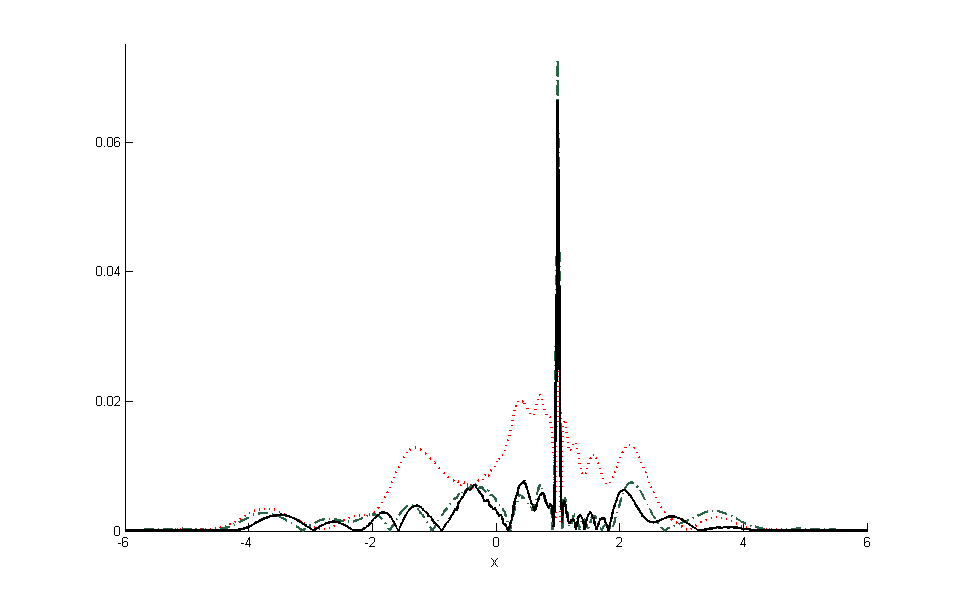
Figure 2 represents the corrected estimator for K=0K=0 and K=1K=1 and the oracle. All the estimators are evaluated on the same trajectory. They manage to reproduce the shape of the density ff. As expected the oracle looks better than the other two and the uncorrected (K=0K=0) seems to make larger errors than the 1-corrected in estimating ff. Figure 3 represents for every values in [−6,6][-6,6] the absolute distance between those estimators –evaluated on the same trajectory– and the true density ff. Therefore it enables to determine in which area an estimator fails to estimate ff and to get an idea of the error made. The graphic was obtained after M=1000M=1000 Monte-Carlo simulations of each estimator and averaging the results. The uncorrected estimator is not as good as the estimator corrected at order 1. The oracle and the estimator corrected at order 1 seem to have similar performances. Each of the estimators makes larger errors around 11 which is where the density ff is peaked.

Refer to caption
Figure 2: Estimators of the density ff (plain grey) for T=10000T=10000 and Δ=0.1\Delta=0.1: the uncorrected (dotted red), the 1-corrected (dashed green) and the oracle (plain dark).
Refer to caption
Figure 3: Mean absolute error between the estimators and the true density (M=1000, T=10000T=10000 and Δ=0.1\Delta=0.1): the uncorrected (dotted red), the 1-corrected (dashed green) and the oracle (plain dark).

Evaluation of the L2L_{2} errors enables to confirm the former graphical observation. We approximate the L2L_{2} errors by Monte Carlo. For that we compute M=1000M=1000 times each estimator (for T=10000T=10000 and Δ=0.1\Delta=0.1) and approximate the L2L_{2} loss by

1M​∑i=1M(∑p=01200(f^​(−6+0.01​p)−f⁡(−6+0.01​p))2×0.01),\frac{1}{M}\sum_{i=1}^{M}\Big(\sum_{p=0}^{1200}\big(\widehat{f}(-6+0.01p)-f(-6+0.01p)\big)^{2}\times 0.01\Big),

where f^\widehat{f} is one of the estimators. For each Monte Carlo iteration the corrected and oracle estimators are evaluated on the same trajectory. The results are reproduced in the following table.

Estimator Oracle K=0K=0 K=1K=1 K=2K=2 K=3K=3
L2L_{2} error (×10−4\times 10^{-4}) 0.1117 0.1842 0.1353 0.1350 0.1350
Standard deviation (×10−5\times 10^{-5}) 0.3495 0.4434 0.4363 0.4366 0.4366

This confirms that there is an actual gain in considering the estimator corrected at order 1 instead of the uncorrected one. In the following table we estimate the (pm​(Δ))\big(p_{m}(\Delta)\big) defined in Proposition 1.

Estimated quantity p1^\widehat{p_{1}} p2^\widehat{p_{2}} p3^\widehat{p_{3}}
Estimation 0.9508 0.0476 0.0016
Standard deviation 0.0022 0.0022 0.0004

It turns out that without the correction we estimate the density ff on a data set where 5%5\% of the observations are realisations of a law which is not ff. This explains why it is relevant to take them into account when estimating ff. Considering more than 1 or 2 corrections is unnecessary as the L2L_{2} losses get stable afterwards. The L2L_{2} loss of the oracle is strictly lower than the loss of the estimator corrected at order KK, even for large KK. That difference is explained by the fact that to estimate the mmth convolution power we do not use NTN_{T} data points but NT,m=⌊NT/m⌋N_{T,m}=\lfloor N_{T}/m\rfloor. Therefore we do not loose in terms of rate of convergence, but we surely deteriorate the constants in comparison with the oracle. Numerical results are consistent with the theoretical results of Theorem 1 where we proved a rate of convergence for the estimator corrected at order KK in

max⁡{T−α⁡(s,p,π),ΔTK+1}.\max\big\{T^{-{\alpha(s,p,\pi)}},\Delta_{T}^{K+1}\big\}.

Since α⁡(s,p,π)≤1/2{\alpha(s,p,\pi)}\leq 1/2, the rate decreases with KK and becomes stable once ΔT2​K+2​T≤ℭ\Delta_{T}^{2K+2}T\leq\mathfrak{C}. In the numerical example we took T=10000T=10000 and Δ=0.1\Delta=0.1 thus T​Δ4=1T\Delta^{4}=1 which explains why in the example we did not observe improvements when correcting with KK greater than 2.

4 Discussion

4.1 Relation to other works

A compound Poisson process is a pure jump Lévy process and can be studied accordingly using Lévy-Kintchine formula. Estimating the jump density ff is then equivalent to estimating the Lévy measure since for compound Poisson process it is the product ϑ​f​(x)​d​x\vartheta f(x)dx. A possible estimation strategy in that case is to provide an estimator of the Fourier transform of the density. That strategy is quite different from the one introduced in this paper but is usually adopted when estimating the compound law of a compound Poisson process (see Figueroa-López [10], Comte and Genon-Catalot [4, 6] or Bec and Lacour [1]).

The nonparametric estimation of the Lévy measure from the discrete observation of a pure jump Lévy process from high frequency data (which corresponds to our microscopic regime ΔT→0\Delta_{T}\rightarrow 0) has been studied in great detail by Comte and Genon-Catalot [4, 6] and Figueroa-López [10]. In [10] the nonparametric estimation of the Lévy density is made via a sieve estimator. They show that it attains minimax rates of convergence for the L2L_{2} loss uniformly over a class of Besov functions for a sampling size ΔT\Delta_{T} such that –with our notation– T​ΔT≤1T\Delta_{T}\leq 1. Comte and Genon-Catalot [4, 6] construct an adaptive nonparametric estimator of the Lévy measure, which attains minimax rates of convergence on Sobolev spaces for the L2L_{2} loss for a sampling size ΔT\Delta_{T} such that T​ΔT≤1T\Delta_{T}\leq 1 (or T​ΔT2≤1T\Delta_{T}^{2}\leq 1 under smoother assumptions). Bec and Lacour [1] obtained similar results when T​ΔT2≤1T\Delta_{T}^{2}\leq 1. The statistical setting of [6] is more general since they estimate the Lévy measure from observations of a Lévy process with a Brownian component.

Our result is limited to the Poisson case contrary to Bec and Lacour [1], Comte and Genon-Catalot [4] and Figueroa-López [10] who worked on the larger class of pure jump Lévy processes. However in the case of a Poisson process we generalise them since we provide an adaptive density estimator which attains minimax rates of convergence, for the LpL_{p} loss, p≥1p\geq 1, uniformly over Besov balls for regime where ΔT\Delta_{T} is polynomially slow. If ΔT\Delta_{T} decays even slower, for instance logarithmically in TT, we still have an upper bound for the rate of convergence of our estimator.

4.2 Possible extensions

In this paper we give an adaptive minimax procedure for the estimation of the compound density of a compound Poisson process in the microscopic regime. The same estimation problem in an intermediate regime, namely when the process is observed at a sampling rate Δ>0\Delta>0 fixed, has been studied in van Es et al. [20] and in the more general setting of Lévy processes by Comte and Genon-Catalot [5] and Reiß [18]. van Es et al. [20] provide a consistent kernel density estimator of the compound density of a compound Poisson process of known intensity. They also focus on the nonzero increments for the estimation, but sidestep the problem of the random number of data NTN_{T} by assuming that they have a sample of a given size.

The estimator corrected at order KK presented here should extend to intermediate regime where ΔT→Δ∞<1\Delta_{T}\rightarrow\Delta_{\infty}<1 and the rate of convergence given in Theorem 1 should generalise in

max⁡{T−α⁡(s,p,π),Δ∞K+1}.\max\big\{T^{-{\alpha(s,p,\pi)}},\Delta_{\infty}^{K+1}\big\}.

An improvement of the results would be the estimation of the compound density of renewal reward processes, or Continuous Time Random Walk, where it is no longer imposed that the elapsed time between jumps is exponentially distributed. Then the Lévy property is lost, the increments of the renewal process are no longer independent nor identically distributed. An estimation strategy based on the Lévy-Kintchine formula is not possible. Such processes enable to model random phenomena where the elapse time between events is not memoryless; they have many applications for instance in finance (see Meerschaert et al. [16]), in biology (see Fedotov et al. [9]) or for modelling earthquakes (see Helmstetter et al. [12]).

5 Proof of Theorem 1

In the sequel ℭ\mathfrak{C} denotes a generic constant which may vary from line to line. Its dependencies may be indicated in the index.

5.1 Proof of part 1) of Theorem 1

Preliminary lemmas

To prove part 1) of Theorem 1 we apply the general results of Kerkyacharian and Picard [14]. For that we establish some technical lemmas.

Lemma 2.

If ff belongs to ℱ⁡(s,π,𝔐)\mathcal{F}(s,{\pi},\mathfrak{M}) then for m≥1m\geq 1, 𝐏Δ​[f]⋆m\mathbf{P}_{\Delta}[f]^{\star m} also belongs to ℱ⁡(s,π,𝔐)\mathcal{F}(s,{\pi},\mathfrak{M}).

Proof of Lemma 2.

It is straightforward to derive ‖𝐏Δ​[f]⋆m‖L1​(ℝ)=1\big\|\mathbf{P}_{\Delta}[f]^{\star m}\big\|_{L_{1}(\mathbb{R})}=1. The remainder of the proof is a consequence of the following result: Let f∈ℬπ​∞sf\in\mathcal{B}^{s}_{{\pi}\infty} and g∈L1g\in L_{1} we have

‖f⋆g‖s​π​∞≤‖f‖s​π​∞​‖g‖L1​(ℝ).\displaystyle\|f\star g\|_{s{\pi}\infty}\leq\|f\|_{s{\pi}\infty}\|g\|_{L_{1}(\mathbb{R})}. (♢\diamondsuit)

To prove the ( ♢ ‣ 5.1) we use the following norm which is equivalent to the Besov norm (see [11])

‖ν‖s​π​∞=‖ν‖Lπ​(ℝ)+‖ν(n)‖Lπ​(ℝ)+‖wπ2​(ν(n),t)ta‖∞\displaystyle\|\nu\|_{s{\pi}\infty}=\|\nu\|_{L_{\pi}(\mathbb{R})}+\|\nu^{(n)}\|_{L_{\pi}(\mathbb{R})}+\Big\|\frac{w_{\pi}^{2}(\nu^{(n)},t)}{t^{a}}\Big\|_{\infty} (17)

where s=n+as=n+a, n∈ℕn\in\mathbb{N} and a∈(0,1]a\in(0,1], and ww is the modulus of continuity

wπ2​(ν,t)=sup|h|≤t​‖𝐃h​𝐃h​[ν]‖Lπ​(ℝ),w_{\pi}^{2}(\nu,t)=\underset{|h|\leq t}{\sup}\big\|\mathbf{D}^{h}\mathbf{D}^{h}[\nu]\big\|_{L_{\pi}(\mathbb{R})},

where 𝐃h​[ν]​(x)=ν⁡(x−h)−ν⁡(x)\mathbf{D}^{h}[\nu](x)=\nu(x-h)-\nu(x). The result is a consequence of Young’s inequality and elementary properties of the convolution product. We use the definition (17) of the norm and treat each term separately. First Young’s inequality gives

‖f1⋆f2‖Lπ​(ℝ)≤‖f1‖Lπ​(ℝ)​‖f2‖L1​(ℝ).\displaystyle\|f_{1}\star f_{2}\|_{L_{\pi}(\mathbb{R})}\leq\|f_{1}\|_{L_{\pi}(\mathbb{R})}\|f_{2}\|_{L_{1}(\mathbb{R})}. (18)

Then the differentiation property of the convolution product leads for n≥1n\geq 1 to

‖dnd​xn​(f1⋆f2)‖Lπ​(ℝ)=‖(dnd​xn​f1)⋆f2‖Lπ​(ℝ)≤‖dnd​xn​f1‖Lπ​(ℝ)​‖f2‖L1​(ℝ).\displaystyle\Big\|\frac{d^{n}}{dx^{n}}(f_{1}\star f_{2})\Big\|_{L_{\pi}(\mathbb{R})}=\Big\|\Big(\frac{d^{n}}{dx^{n}}f_{1}\Big)\star f_{2}\Big\|_{L_{\pi}(\mathbb{R})}\leq\Big\|\frac{d^{n}}{dx^{n}}f_{1}\Big\|_{L_{\pi}(\mathbb{R})}\|f_{2}\|_{L_{1}(\mathbb{R})}. (19)

Finally translation invariance of the convolution product enables to get

‖𝐃h​𝐃h​[(f1⋆f2)(n)]‖Lπ​(ℝ)\displaystyle\big\|\mathbf{D}^{h}\mathbf{D}^{h}[(f_{1}\star f_{2})^{(n)}]\big\|_{L_{\pi}(\mathbb{R})} =‖(𝐃h​𝐃h​[f1(n)])⋆f2‖Lπ​(ℝ)\displaystyle=\big\|(\mathbf{D}^{h}\mathbf{D}^{h}[f_{1}^{(n)}])\star f_{2}\big\|_{L_{\pi}(\mathbb{R})}
≤‖𝐃h​𝐃h​[f1(n)]‖Lπ​(ℝ)​‖f2‖L1​(ℝ).\displaystyle\leq\big\|\mathbf{D}^{h}\mathbf{D}^{h}[f_{1}^{(n)}]\big\|_{L_{\pi}(\mathbb{R})}\|f_{2}\|_{L_{1}(\mathbb{R})}. (20)

Inequality ( ♢ ‣ 5.1) is then obtained by bounding (17) with (18), (19) and (20) lead to the result. To complete the proof of Lemma 2, we apply m−1m-1 times ( ♢ ‣ 5.1) which leads to

∀m∈ℕ∖{0},‖𝐏Δ​[f]⋆m‖s​π​∞≤‖𝐏Δ​[f]‖s​π​∞.\forall m\in\mathbb{N}\setminus\{0\},\ \ \ \ \ \big\|\mathbf{P}_{\Delta}[f]^{\star m}\big\|_{s{\pi}\infty}\leq\big\|\mathbf{P}_{\Delta}[f]\big\|_{s{\pi}\infty}.

The triangle inequality gives ‖𝐏Δ​[f]⋆m‖s​π​∞≤‖f‖s​π​∞≤𝔐\|\mathbf{P}_{\Delta}[f]^{\star m}\|_{s{\pi}\infty}\leq\|f\|_{s{\pi}\infty}\leq\mathfrak{M} which concludes the proof. ∎

Lemma 3.

Let 2j≤NT2^{j}\leq N_{T} then for all m∈ℕ∖{0}m\in\mathbb{N}\setminus\{0\} and for p≥1p\geq 1 we have

𝔼[|γ^j​k(m)−γj​k(m)|p|NT]≤ℭp,m,‖g‖Lp​(ℝ),𝔐,ϑNT−p/2,\mathbb{E}\big[\big|\widehat{\gamma}_{jk}^{(m)}-\gamma_{jk}^{(m)}\big|^{p}\big|N_{T}\big]\leq\mathfrak{C}_{p,m,\|g\|_{L_{p}(\mathbb{R})},\mathfrak{M},\vartheta}N_{T}^{-p/2},

where γ^j​k(m)\widehat{\gamma}_{jk}^{(m)} is defined in (12) and

γj​k(m)=∫gj​k​(y)​𝐏Δ​[f]⋆m​(y)​𝑑y.\displaystyle\gamma_{jk}^{(m)}=\int g_{jk}(y)\mathbf{P}_{\Delta}[f]^{\star m}(y)dy. (21)
Proof of Lemma 3.

The proof is obtained with Rosenthal’s inequality: let p≥1p\geq 1 and let (Y1,…,Yn)(Y_{1},\ldots,Y_{n}) be independent random variables such that 𝔼⁡[Yi]=0\mathbb{E}[Y_{i}]=0 and 𝔼⁡[|Yi|p]<∞\mathbb{E}\big[|Y_{i}|^{p}\big]<\infty. Then there exists ℭp\mathfrak{C}_{p} such that

𝔼⁡[|∑i=1nYi|p]≤ℭp​{∑i=1n𝔼⁡[|Yi|p]+(∑i=1n𝔼⁡[|Yi|2])p/2}.\displaystyle\mathbb{E}\bigg[\Big|\sum_{i=1}^{n}Y_{i}\Big|^{p}\bigg]\leq\mathfrak{C}_{p}\bigg\{\sum_{i=1}^{n}\mathbb{E}\big[|Y_{i}|^{p}\big]+\Big(\sum_{i=1}^{n}\mathbb{E}\big[|Y_{i}|^{2}\big]\Big)^{p/2}\bigg\}. (22)

The (𝐃mΔT​XSi)\big(\mathbf{D}^{\Delta_{T}}_{m}X_{S_{i}}\big) are independent and identically distributed with common density 𝐏ΔT​[f]⋆m\mathbf{P}_{\Delta_{T}}[f]^{\star m} and 𝔼⁡[γ^j​k(m)]=γj​k(m).\mathbb{E}[\widehat{\gamma}_{jk}^{(m)}]=\gamma_{jk}^{(m)}. Then γ^j​k(m)−γj​k(m)\widehat{\gamma}_{jk}^{(m)}-\gamma_{jk}^{(m)} is a sum of NT,m=⌊NT/m⌋N_{T,m}=\lfloor N_{T}/m\rfloor centered, independent and identically distributed random variables. It follows that

𝔼⁡[|gj​k​(𝐃mΔT​XSi)|p]\displaystyle\mathbb{E}\big[\big|g_{jk}(\mathbf{D}^{\Delta_{T}}_{m}X_{S_{i}})\big|^{p}\big] ≤2p​2j​p/2​∫|g⁡(2j​y−k)|p​𝐏ΔT​[f]⋆m​(y)​𝑑y\displaystyle\leq 2^{p}2^{jp/2}\int|g(2^{j}y-k)|^{p}\mathbf{P}_{\Delta_{T}}[f]^{\star m}(y)dy
=2p​2j⁡(p/2−1)​∫|g⁡(z)|p​𝐏ΔT​[f]⋆m​(z+k2j)​𝑑z\displaystyle=2^{p}2^{j(p/2-1)}\int|g(z)|^{p}\mathbf{P}_{\Delta_{T}}[f]^{\star m}\Big(\frac{z+k}{2^{j}}\Big)dz
≤2p​2j⁡(p/2−1)​‖g‖Lp​(ℝ)p​‖𝐏ΔT​[f]⋆m‖∞,\displaystyle\leq 2^{p}2^{j(p/2-1)}\|g\|_{L_{p}(\mathbb{R})}^{p}\big\|\mathbf{P}_{\Delta_{T}}[f]^{\star m}\big\|_{\infty},

where we made the substitution z=2j​x−kz=2^{j}x-k. To control ‖𝐏ΔT​[f]⋆m‖∞\|\mathbf{P}_{\Delta_{T}}[f]^{\star m}\|_{\infty} we use the Sobolev embeddings (see [3, 7, 11])

ℬπ​∞s↪ℬp​∞s′ and ℬπ​∞s′↪ℬ∞​∞s,\displaystyle\mathcal{B}^{s}_{{\pi}\infty}\hookrightarrow\mathcal{B}^{s^{\prime}}_{p\infty}\ \ \ \mbox{ and }\ \ \ \mathcal{B}^{s^{\prime}}_{{\pi}\infty}\hookrightarrow\mathcal{B}^{s}_{{\infty}\infty}, (23)

where p>πp>\pi, s​π>1s\pi>1 and s′=s−1/π+1/ps^{\prime}=s-1/\pi+1/p, it follows that

‖𝐏ΔT​[f]⋆m‖∞≤ℭs,π​‖𝐏ΔT​[f]⋆m‖ℬπ​∞​(𝒟)s.\|\mathbf{P}_{\Delta_{T}}[f]^{\star m}\|_{\infty}\leq\mathfrak{C}_{s,\pi}\|\mathbf{P}_{\Delta_{T}}[f]^{\star m}\|_{\mathcal{B}^{s}_{\pi\infty(\mathcal{D})}}.

We deduce from Lemma 2 that ‖𝐏ΔT​[f]⋆m‖∞≤ℭs,π​𝔐\|\mathbf{P}_{\Delta_{T}}[f]^{\star m}\|_{\infty}\leq\mathfrak{C}_{s,\pi}\mathfrak{M}. We get

𝔼⁡[|gj​k​(𝐃mΔT​XSi)|p]≤2p​2j⁡(p/2−1)​‖g‖Lp​(ℝ)p​𝔐\mathbb{E}\big[\big|g_{jk}(\mathbf{D}^{\Delta_{T}}_{m}X_{S_{i}})\big|^{p}\big]\leq 2^{p}2^{j(p/2-1)}\|g\|_{L_{p}(\mathbb{R})}^{p}\mathfrak{M}

and 𝔼⁡[|gj​k​(𝐃mΔT​XSi)|2]≤𝔐\mathbb{E}\big[\big|g_{jk}(\mathbf{D}^{\Delta_{T}}_{m}X_{S_{i}})\big|^{2}\big]\leq\mathfrak{M} since ‖g‖22=1\|g\|_{2}^{2}=1.

The accept-reject algorithm ensures that for all n≥1n\geq 1 the increments (𝐃ΔT​XS1,…,𝐃ΔT​XSn)\big(\mathbf{D}^{\Delta_{T}}X_{S_{1}},\ldots,\mathbf{D}^{\Delta_{T}}X_{S_{n}}\big) are independent of NTN_{T} and then NT,mN_{T,m}. Indeed the (𝐃ΔT​Xi,i=1,…,⌊T​ΔT−1⌋)\big(\mathbf{D}^{\Delta_{T}}X_{i},i=1,\ldots,\lfloor T\Delta_{T}^{-1}\rfloor\big) are independent and identically distributed and the (𝐃ΔT​XSi)\big(\mathbf{D}^{\Delta_{T}}X_{S_{i}}\big) are constructed with Si=inf{j>Si−1,𝐃ΔT​Xj≠0}.S_{i}=\inf\big\{j>S_{i-1},\mathbf{D}^{\Delta_{T}}X_{j}\neq 0\big\}. Therefore we can apply Rosenthal’s inequality conditional on NTN_{T} to γ^j​k(m)−γj​k(m)\widehat{\gamma}_{jk}^{(m)}-\gamma_{jk}^{(m)} and derive for p≥1p\geq 1

𝔼⁡[|γ^j​k(m)−γj​k(m)|p|NT]\displaystyle\mathbb{E}\big[\big|\widehat{\gamma}_{jk}^{(m)}-\gamma_{jk}^{(m)}\big|^{p}\big|N_{T}\big] ≤ℭp{2p(2jNT,m)p/2−1∥g∥Lp​(ℝ)p𝔐+𝔐p/2}NT,m−p/2.\displaystyle\leq\mathfrak{C}_{p}\Big\{2^{p}\Big(\frac{2^{j}}{N_{T,m}}\Big)^{p/2-1}\|g\|_{L_{p}(\mathbb{R})}^{p}\mathfrak{M}+\mathfrak{M}^{p/2}\Big\}N_{T,m}^{-p/2}.

This concludes the proof.∎

Lemma 4.

Choose jj and cc such that

2j​NT−1​log⁡(NT1/2)≤1​ and ​c2≥16​m3​(𝔐+c​‖g‖∞6).2^{j}N_{T}^{-1}\log\big(N_{T}^{1/2}\big)\leq 1\mbox{ and }c^{2}\geq\frac{16m}{3}\Big(\mathfrak{M}+\frac{c\|g\|_{\infty}}{6}\Big).

For all m∈ℕ∖{0}m\in\mathbb{N}\setminus\{0\} and r≥1r\geq 1 let κr=c​r\kappa_{r}=cr. We have

ℙ(|γ^j​k(m)−γj​k(m)|≥κr2NT−1/2log⁡(NT1/2)|NT)≤NT−r/2,\mathbb{P}\Big(|\widehat{\gamma}_{jk}^{(m)}-\gamma_{jk}^{(m)}|\geq\frac{\kappa_{r}}{2}N_{T}^{-1/2}\sqrt{\log\big(N_{T}^{1/2}\big)}\Big|N_{T}\Big)\leq N_{T}^{-r/2},

where γ^j​k(m)\widehat{\gamma}_{jk}^{(m)} is defined in (12) and γj​k(m)\gamma_{jk}^{(m)} in (21).

Proof of Lemma 4.

The proof is obtained with Bernstein’s inequality. Consider Y1,…,YnY_{1},\ldots,Y_{n} independent random variables such that |Yi|≤𝔄|Y_{i}|\leq\mathfrak{A}, 𝔼⁡[Yi]=0\mathbb{E}[Y_{i}]=0 and bn2=∑i=1n𝔼⁡[Yi2]b_{n}^{2}=\sum_{i=1}^{n}\mathbb{E}[Y_{i}^{2}]. Then for any λ>0\lambda>0,

ℙ⁡(|∑i=1nYi|>λ)≤2​exp⁡(−λ22​(bn2+λ​𝔄3)).\displaystyle\mathbb{P}\Big(\Big|\sum_{i=1}^{n}Y_{i}\Big|>\lambda\Big)\leq 2\exp\Big(-\frac{\lambda^{2}}{2(b_{n}^{2}+\frac{\lambda\mathfrak{A}}{3})}\Big). (24)

For all m≥1m\geq 1, γ^j​k(m)−γj​k(m)\widehat{\gamma}_{jk}^{(m)}-\gamma_{jk}^{(m)} is a sum of NT,m=⌊NT/m⌋N_{T,m}=\lfloor N_{T}/m\rfloor centered independent and identically distributed random variables bounded by 2j/2​‖g‖∞2^{j/2}\|g\|_{\infty} and 𝔼⁡[|gj​k​(𝐃mΔT​XSi)|2]≤𝔐.\mathbb{E}\big[\big|g_{jk}(\mathbf{D}^{\Delta_{T}}_{m}X_{S_{i}})\big|^{2}\big]\leq\mathfrak{M}. The accept-reject algorithm ensures that for all n≥1n\geq 1 the increments (𝐃ΔT​XS1,…,𝐃ΔT​XSn)\big(\mathbf{D}^{\Delta_{T}}X_{S_{1}},\ldots,\mathbf{D}^{\Delta_{T}}X_{S_{n}}\big) are independent of NTN_{T} (see proof of Lemma 3), we apply Bernstein’s inequality conditional on NTN_{T}. We have

ℙ(|γ^j​k(m)\displaystyle\mathbb{P}\Big(|\widehat{\gamma}_{jk}^{(m)} −γj​k(m)|≥κr2NT−1/2log⁡(NT1/2)|NT)\displaystyle-\gamma_{jk}^{(m)}|\geq\frac{\kappa_{r}}{2}N_{T}^{-1/2}\sqrt{\log\big(N_{T}^{1/2}\big)}\Big|N_{T}\Big)
≤\displaystyle\leq 2​exp⁡(−κr2​NT−1​log⁡(NT1/2)​NT,m28​(NT,m​𝔐+κrNT,mNT−1/2log⁡(NT1/2)2j/2∥g∥∞6))\displaystyle 2\exp\Bigg(-\frac{\kappa_{r}^{2}N_{T}^{-1}\log\big(N_{T}^{1/2}\big)N_{T,m}^{2}}{8\Big(N_{T,m}\mathfrak{M}+\frac{\kappa_{r}N_{T,m}N_{T}^{-1/2}\sqrt{\log\big(N_{T}^{1/2}\big)}2^{j/2}\|g\|_{\infty}}{6}\Big)}\Bigg)
=\displaystyle= 2​exp⁡(−c2​r​NT−1​NT,m8​(𝔐+κrNT−1/2log⁡(NT1/2)2j/2∥g∥∞6)​r​log⁡(NT1/2)).\displaystyle 2\exp\Bigg(-\frac{c^{2}rN_{T}^{-1}N_{T,m}}{8\Big(\mathfrak{M}+\frac{\kappa_{r}N_{T}^{-1/2}\sqrt{\log\big(N_{T}^{1/2}\big)}2^{j/2}\|g\|_{\infty}}{6}\Big)}r\log\big(N_{T}^{1/2}\big)\Bigg).

Using that

m​NT−1​NT,m=mNT​⌊NTm⌋≥32,mN_{T}^{-1}N_{T,m}=\frac{m}{N_{T}}\Big\lfloor\frac{N_{T}}{m}\Big\rfloor\geq\frac{3}{2},

for TT large enough and 2j/2​NT−1​log⁡(NT1/2)≤12^{j/2}N_{T}^{-1}\sqrt{\log\big(N_{T}^{1/2}\big)}\leq 1 it follows that

ℙ(|γ^j​k(m)−γj​k(m)\displaystyle\mathbb{P}\Big(|\widehat{\gamma}_{jk}^{(m)}-\gamma_{jk}^{(m)} |≥κr2NT−1/2log⁡(NT1/2)|NT)\displaystyle|\geq\frac{\kappa_{r}}{2}N_{T}^{-1/2}\sqrt{\log\big(N_{T}^{1/2}\big)}\Big|N_{T}\Big)
≤2​exp⁡(−3​c2​r16​m​(𝔐+κr​‖g‖∞6)​r​log⁡(NT1/2)).\displaystyle\leq 2\exp\Bigg(-\frac{3c^{2}r}{16m\big(\mathfrak{M}+\frac{\kappa_{r}\|g\|_{\infty}}{6}\big)}r\log\big(N_{T}^{1/2}\big)\Bigg).

With c2≥16​m3​(𝔐+c​‖g‖∞6)c^{2}\geq\frac{16m}{3}\big(\mathfrak{M}+\frac{c\|g\|_{\infty}}{6}\big) we get

ℙ(|γ^j​k(m)−γj​k(m)\displaystyle\mathbb{P}\Big(|\widehat{\gamma}_{jk}^{(m)}-\gamma_{jk}^{(m)} |≥κr2NT−1/2log⁡(NT1/2)|NT)≤NT−r/2.\displaystyle|\geq\frac{\kappa_{r}}{2}N_{T}^{-1/2}\sqrt{\log\big(N_{T}^{1/2}\big)}\Big|N_{T}\Big)\leq N_{T}^{-r/2}.

The proof is complete.∎

Completion of proof of part 1) of Theorem 1

Part 1) of Theorem 1 is a consequence of Lemma 2, 3, 4 and of the general theory of wavelet threshold estimators of [14]. It suffices to have conditions (5.1) and (5.2) of Theorem 5.1 of [14], which are satisfied –Lemma 3 and 4– with c(T)=NT−1/2c(T)=N_{T}^{-1/2} and Λn=c​(T)−1\Lambda_{n}=c(T)^{-1} (with the notations of [14]). We can now apply Theorem 5.1, its Corollary 5.1 and Theorem 6.1 of [14] to obtain the result.

5.2 Proof of part 2) of Theorem 1

Preliminary result

The result of part 1) of Theorem 1 where given conditional on NTN_{T}. To prove part 2) we replace NTN_{T} by its deterministic counterpart. We introduce the following result.

Proposition 2.

For all r>0r>0, there exist 1≤ℭϑ<∞,1\leq\mathfrak{C}_{\vartheta}<\infty, where ϑ→ℭϑ\vartheta\rightarrow\mathfrak{C}_{\vartheta} is continuous, such that

1/ℭϑ​T−r≤𝔼⁡[NT−r]\displaystyle 1/\mathfrak{C}_{\vartheta}T^{-r}\leq\mathbb{E}\big[N_{T}^{-r}\big] ≤ℭϑ​T−r.\displaystyle\leq\mathfrak{C}_{\vartheta}T^{-r}.
Proof of Proposition 2.

We have

NT=∑i=1⌊T​ΔT−1⌋𝟙{𝐃ΔTXi≠0},N_{T}=\sum_{i=1}^{\lfloor T\Delta_{T}^{-1}\rfloor}\mathds{1}_{\{\mathbf{D}^{\Delta_{T}}X_{i}\neq 0\}},

where

𝔼[𝟙{𝐃ΔTXi≠0}]=p(ΔT)=1−exp(−ϑΔT).\mathbb{E}\big[\mathds{1}_{\{\mathbf{D}^{\Delta_{T}}X_{i}\neq 0\}}\big]=p(\Delta_{T})=1-\exp(-\vartheta\Delta_{T}).

Introduce Yi=𝟙{𝐃ΔTXi≠0}−p(ΔT)Y_{i}=\mathds{1}_{\{\mathbf{D}^{\Delta_{T}}X_{i}\neq 0\}}-p(\Delta_{T}), the YiY_{i} are centered independent and identically distributed random variables bounded by 2 and 𝔼⁡[Yi2]≤p⁡(ΔT)\mathbb{E}[Y_{i}^{2}]\leq p(\Delta_{T}), it follows from Bernstein’s inequality (24) that for λ>0\lambda>0

ℙ⁡(|NT⌊T​ΔT−1⌋−p⁡(ΔT)|>λ)\displaystyle\mathbb{P}\Big(\Big|\frac{N_{T}}{\lfloor T\Delta_{T}^{-1}\rfloor}-p(\Delta_{T})\Big|>\lambda\Big) ≤exp⁡(−⌊T​ΔT−1⌋​λ22​(p​(ΔT)+2​λ3)).\displaystyle\leq\exp\bigg(-\frac{\lfloor T\Delta_{T}^{-1}\rfloor\lambda^{2}}{2\big(p(\Delta_{T})+\frac{2\lambda}{3}\big)}\bigg). (25)

We choose λ=p⁡(ΔT)/2\lambda=p(\Delta_{T})/2, on the set {|NT⌊T​ΔT−1⌋−p(ΔT)|≤λ}\big\{\big|\frac{N_{T}}{\lfloor T\Delta_{T}^{-1}\rfloor}-p(\Delta_{T})\big|\leq\lambda\big\} we have

⌊T​ΔT−1⌋​p⁡(ΔT)2≤NT≤⌊T​ΔT−1⌋​3​p​(ΔT)2.\lfloor T\Delta_{T}^{-1}\rfloor\frac{p(\Delta_{T})}{2}\leq N_{T}\leq\lfloor T\Delta_{T}^{-1}\rfloor\frac{3p(\Delta_{T})}{2}.

Moreover for ΔT\Delta_{T} small enough we have that

ϑ2≤p⁡(ΔT)=1−exp⁡(−ϑ​ΔT)≤ϑ​ΔT.\frac{\vartheta}{2}\leq p(\Delta_{T})=1-\exp(-\vartheta\Delta_{T})\leq\vartheta\Delta_{T}.

We have for all λ>0\lambda>0

𝔼⁡[NT−r]\displaystyle\mathbb{E}\big[N_{T}^{-r}\big] =𝔼[NT−r𝟙{|NT⌊T​ΔT−1⌋−p(ΔT)|>λ}]+𝔼[NT−r𝟙{|NT⌊T​ΔT−1⌋−p(ΔT)|≤λ}].\displaystyle=\mathbb{E}\Big[N_{T}^{-r}\mathds{1}_{\big\{|\frac{N_{T}}{\lfloor T\Delta_{T}^{-1}\rfloor}-p(\Delta_{T})|>\lambda\big\}}\Big]+\mathbb{E}\Big[N_{T}^{-r}\mathds{1}_{\big\{|\frac{N_{T}}{\lfloor T\Delta_{T}^{-1}\rfloor}-p(\Delta_{T})|\leq\lambda\big\}}\Big].

Since for r>0r>0 the function x→x−rx\rightarrow x^{-r} is decreasing and NT≥1N_{T}\geq 1 we have using (25) the upper bound

𝔼⁡[NT−r]\displaystyle\mathbb{E}\big[N_{T}^{-r}\big] ≤ℙ⁡(|NT⌊T​ΔT−1⌋−p⁡(ΔT)|>p⁡(ΔT)2)+(⌊T​ΔT−1⌋​p​(ΔT)2)−r\displaystyle\leq\mathbb{P}\Big(\Big|\frac{N_{T}}{\lfloor T\Delta_{T}^{-1}\rfloor}-p(\Delta_{T})\Big|>\frac{p(\Delta_{T})}{2}\Big)+\Big(\frac{\lfloor T\Delta_{T}^{-1}\rfloor p(\Delta_{T})}{2}\Big)^{-r}
≤exp⁡(−⌊T​ΔT−1⌋​p​(ΔT)28​(p​(ΔT)+p⁡(ΔT)3))+(⌊T​ΔT−1⌋​p​(ΔT)2)−r\displaystyle\leq\exp\bigg(-\frac{\lfloor T\Delta_{T}^{-1}\rfloor p(\Delta_{T})^{2}}{8\big(p(\Delta_{T})+\frac{p(\Delta_{T})}{3}\big)}\bigg)+\Big(\frac{\lfloor T\Delta_{T}^{-1}\rfloor p(\Delta_{T})}{2}\Big)^{-r}
≤exp⁡(−3​ϑ64​T)+(T​ϑ4)−r.\displaystyle\leq\exp\bigg(-\frac{3\vartheta}{64}T\bigg)+\Big(\frac{T\vartheta}{4}\Big)^{-r}.

For the lower bound we have

𝔼⁡[NT−r]\displaystyle\mathbb{E}\big[N_{T}^{-r}\big] ≥(3​⌊T​ΔT−1⌋​p​(ΔT)2)−r≥(3​T​ϑ2)−r.\displaystyle\geq\Big(\frac{3\lfloor T\Delta_{T}^{-1}\rfloor p(\Delta_{T})}{2}\Big)^{-r}\geq\Big(\frac{3T\vartheta}{2}\Big)^{-r}.

Then there exists 1≤ℭϑ<∞1\leq\mathfrak{C}_{\vartheta}<\infty with ϑ→ℭϑ\vartheta\rightarrow\mathfrak{C}_{\vartheta} continuous such that

1/ℭϑ​T−r≤𝔼⁡[NT−r]≤ℭϑ​T−r.1/\mathfrak{C}_{\vartheta}T^{-r}\leq\mathbb{E}\big[N_{T}^{-r}\big]\leq\mathfrak{C}_{\vartheta}T^{-r}.

The proof is now complete.∎

Completion of proof of part 2) of Theorem 1

To prove Theorem 1 we define the quantity for KK in ℕ\mathbb{N} and xx in 𝒟\mathcal{D}

f^T,ΔK​(x)\displaystyle\widehat{f}^{K}_{T,\Delta}(x) =∑m=1K+1(−1)m+1m​(eϑ​Δ−1)mϑ​Δ​PΔ,m^​(x).\displaystyle=\sum_{m=1}^{K+1}\frac{(-1)^{m+1}}{m}\frac{\big(e^{\vartheta\Delta}-1\big)^{m}}{\vartheta\Delta}\widehat{P_{\Delta,m}}(x).

It is the estimator of ff one would compute if ϑ\vartheta were known. We decompose the LpL_{p} error as follows

(𝔼⁡[‖f~T,ΔTK−f‖Lp​(𝒟)p])1/p≤\displaystyle\big(\mathbb{E}\big[\|\widetilde{f}^{K}_{T,\Delta_{T}}-f\|_{L_{p}(\mathcal{D})}^{p}\big]\big)^{1/p}\leq (𝔼⁡[‖f~T,ΔTK−f^T,ΔTK‖Lp​(𝒟)p])1/p\displaystyle\big(\mathbb{E}\big[\|\widetilde{f}^{K}_{T,\Delta_{T}}-\widehat{f}^{K}_{T,\Delta_{T}}\|_{L_{p}(\mathcal{D})}^{p}\big]\big)^{1/p}
+(𝔼⁡[‖f^T,ΔTK−f‖Lp​(𝒟)p])1/p,\displaystyle+\big(\mathbb{E}\big[\|\widehat{f}^{K}_{T,\Delta_{T}}-f\|_{L_{p}(\mathcal{D})}^{p}\big]\big)^{1/p},

and control each term separately.

First we control 𝔼⁡[‖f^T,ΔTK−f‖Lp​(𝒟)p]\mathbb{E}\big[\|\widehat{f}^{K}_{T,\Delta_{T}}-f\|_{L_{p}(\mathcal{D})}^{p}\big], using the triangle inequality we get

(𝔼⁡[‖∑m=1K+1(−1)m+1m​(eϑ​ΔT−1)mϑ​ΔT​PΔT,m^−𝐏ΔT−1​[𝐏ΔT​[f]]‖Lp​(𝒟)p])1/p\displaystyle\Big(\mathbb{E}\Big[\Big\|\sum_{m=1}^{K+1}\frac{(-1)^{m+1}}{m}\frac{\big(e^{\vartheta{\Delta_{T}}}-1\big)^{m}}{\vartheta{\Delta_{T}}}\widehat{P_{\Delta_{T},m}}-\mathbf{P}_{\Delta_{T}}^{-1}\big[\mathbf{P}_{\Delta_{T}}[f]\big]\Big\|_{L_{p}(\mathcal{D})}^{p}\Big]\Big)^{1/p}
≤∑m=1K+1(eϑ​ΔT−1)mm​ϑ​ΔT​(𝔼⁡[‖PΔT,m^−𝐏ΔT​[f]⋆m‖Lp​(𝒟)p])1/p\displaystyle\leq\sum_{m=1}^{K+1}\frac{\big(e^{\vartheta{\Delta_{T}}}-1\big)^{m}}{m\vartheta{\Delta_{T}}}\big(\mathbb{E}\big[\big\|\widehat{P_{\Delta_{T},m}}-\mathbf{P}_{\Delta_{T}}[f]^{\star m}\big\|_{L_{p}(\mathcal{D})}^{p}\big]\big)^{1/p} (26)
+∑m=K+2∞(eϑ​ΔT−1)mm​ϑ​ΔT∥𝐏ΔT[f]⋆m∥Lp​(ℝ).\displaystyle\ \ \ +\sum_{m=K+2}^{\infty}\frac{\big(e^{\vartheta{\Delta_{T}}}-1\big)^{m}}{m\vartheta{\Delta_{T}}}\|\mathbf{P}_{\Delta_{T}}[f]^{\star m}\|_{L_{p}(\mathbb{R})}. (27)

To bound (26) we use part 1) of Theorem 1 in which the supremum is taken over the class {𝐏ΔT[f]⋆m∈ℱ(s,π,𝔐)}\{\mathbf{P}_{\Delta_{T}}[f]^{\star m}\in\mathcal{F}(s,{\pi},\mathfrak{M})\}. With the inclusion

{𝐏ΔT​[f]⋆m,f∈ℱ⁡(s,π,𝔐)}⊂ℱ⁡(s,π,𝔐)\displaystyle\{\mathbf{P}_{\Delta_{T}}[f]^{\star m},f\in\mathcal{F}(s,{\pi},\mathfrak{M})\}\subset\mathcal{F}(s,{\pi},\mathfrak{M})

and Proposition 2 applied with r=α⁡(s,p,π)​p>0,r={\alpha(s,p,\pi)}p>0, we deduce the upper bound for m≥1m\geq 1

𝔼[∥PΔT,m^−𝐏ΔT−1[𝐏ΔT[f]∥Lp​(𝒟)p]\displaystyle\mathbb{E}\big[\big\|\widehat{P_{\Delta_{T},m}}-\mathbf{P}_{\Delta_{T}}^{-1}\big[\mathbf{P}_{\Delta_{T}}[f]\big\|_{L_{p}(\mathcal{D})}^{p}\big] ≤ℭ​𝔼​[NT−α⁡(s,p,π)​p]\displaystyle\leq\mathfrak{C}\mathbb{E}\big[N_{T}^{-{\alpha(s,p,\pi)}p}\big]
≤ℭ​T−α⁡(s,p,π)​p,\displaystyle\leq\mathfrak{C}T^{-{\alpha(s,p,\pi)}p}, (28)

where ℭ\mathfrak{C} depends on (s,π,p,𝔐,ϕ,ψ,K,ϑ)(s,\pi,p,\mathfrak{M},\phi,\psi,K,\vartheta). To bound (27) Young’s inequality and ‖𝐏ΔT​[f]‖L1​(ℝ)=1\big\|\mathbf{P}_{\Delta_{T}}[f]\big\|_{L_{1}(\mathbb{R})}=1 enable to get

‖𝐏ΔT​[f]⋆m‖Lp​(ℝ)≤‖𝐏ΔT​[f]‖Lp​(ℝ) for ​m≥1.\big\|\mathbf{P}_{\Delta_{T}}[f]^{\star m}\big\|_{L_{p}(\mathbb{R})}\leq\big\|\mathbf{P}_{\Delta_{T}}[f]\big\|_{L_{p}(\mathbb{R})}\ \ \ \mbox{ for }m\geq 1.

The triangle inequality leads to ‖𝐏ΔT​[f]‖Lp​(ℝ)≤‖f‖Lp​(ℝ)\big\|\mathbf{P}_{\Delta_{T}}[f]\big\|_{L_{p}(\mathbb{R})}\leq\|f\|_{L_{p}(\mathbb{R})} and we use the Sobolev embeddings (23) to get ‖f‖Lp​(ℝ)≤ℭs,π,p​𝔐\|f\|_{L_{p}(\mathbb{R})}\leq\mathfrak{C}_{s,\pi,p}\mathfrak{M}. We derive the upper bound

∑m=K+2∞1m​(eϑ​ΔT−1)mϑ​ΔT\displaystyle\sum_{m=K+2}^{\infty}\frac{1}{m}\frac{\big(e^{\vartheta{\Delta_{T}}}-1\big)^{m}}{\vartheta{\Delta_{T}}} ‖𝐏ΔT​[f]⋆m‖Lp​(ℝ)\displaystyle\big\|\mathbf{P}_{\Delta_{T}}[f]^{\star m}\big\|_{L_{p}(\mathbb{R})}
≤‖f‖Lp​(ℝ)​∑m=K+2∞1m​(eϑ​ΔT−1)mϑ​ΔT\displaystyle\leq\|f\|_{L_{p}(\mathbb{R})}\sum_{m=K+2}^{\infty}\frac{1}{m}\frac{\big(e^{\vartheta{\Delta_{T}}}-1\big)^{m}}{\vartheta{\Delta_{T}}}
≤ℭK,ϑ,𝔐​ΔTK+1.\displaystyle\leq\mathfrak{C}_{K,\vartheta,\mathfrak{M}}{\Delta_{T}}^{K+1}. (29)

Thus from (28) and (29) we obtain

supf∈ℱ⁡(s,π,𝔐)​(𝔼⁡[‖f^T,ΔTK−f‖Lp​(𝒟)p])1/p\displaystyle\underset{f\in\mathcal{F}(s,{\pi},\mathfrak{M})}{\sup}\big(\mathbb{E}\big[\big\|\widehat{f}^{K}_{T,\Delta_{T}}-f\big\|_{L_{p}(\mathcal{D})}^{p}\big]\big)^{1/p} ≤ℭ​max⁡{T−α⁡(s,p,π),ΔTK+1},\displaystyle\leq\mathfrak{C}\max\big\{T^{-{\alpha(s,p,\pi)}},\Delta_{T}^{K+1}\big\},

where ℭ\mathfrak{C} depends on (s,π,p,𝔐,ϕ,ψ,K,ϑ)(s,\pi,p,\mathfrak{M},\phi,\psi,K,\vartheta). Since ϑ→ℭ\vartheta\rightarrow\mathfrak{C} is continuous we get for p≥1p\geq 1

supϑ∈[𝔗¯,𝔗¯]​supf∈ℱ⁡(s,π,𝔐)​(𝔼⁡[‖f^T,ΔTK−f‖Lp​(𝒟)p])1/p\displaystyle\underset{\vartheta\in[\underline{\mathfrak{T}},\overline{\mathfrak{T}}]}{\sup}\ \underset{f\in\mathcal{F}(s,{\pi},\mathfrak{M})}{\sup}\big(\mathbb{E}\big[\big\|\widehat{f}^{K}_{T,\Delta_{T}}-f\big\|_{L_{p}(\mathcal{D})}^{p}\big]\big)^{1/p} ≤ℭK,𝔐​max⁡{T−α⁡(s,p,π),ΔTK+1},\displaystyle\leq\mathfrak{C}_{K,\mathfrak{M}}\max\big\{T^{-{\alpha(s,p,\pi)}},\Delta_{T}^{K+1}\big\},

where ℭ\mathfrak{C} depends on (s,π,p,𝔐,ϕ,ψ,K)(s,\pi,p,\mathfrak{M},\phi,\psi,K)

We now control 𝔼⁡[‖f~T,ΔTK−f^T,ΔTK‖Lp​(𝒟)p]\mathbb{E}\big[\|\widetilde{f}^{K}_{T,\Delta_{T}}-\widehat{f}^{K}_{T,\Delta_{T}}\|_{L_{p}(\mathcal{D})}^{p}\big] and use (15) to derive

f~T,ΔTK=∑m=1K+1(−1)mm​((1−p^T)−1−1)mlog⁡(1−p^T)​PΔT,m^,\displaystyle\widetilde{f}^{K}_{T,\Delta_{T}}=\sum_{m=1}^{K+1}\frac{(-1)^{m}}{m}\frac{\big((1-\widehat{p}_{T})^{-1}-1\big)^{m}}{\log(1-\widehat{p}_{T})}\widehat{P_{\Delta_{T},m}},

where PΔT,m^\widehat{P_{\Delta_{T},m}} does not depend on ϑ\vartheta (see (12)). Define

Gm​(x)=((1−x)−1−1)mlog⁡(1−x).G_{m}(x)=\frac{((1-x)^{-1}-1)^{m}}{\log(1-x)}.

The triangle inequality leads to

(𝔼[∥f^T,ΔTK(ϑ^)−\displaystyle\big(\mathbb{E}\big[\|\widehat{f}^{K}_{T,\Delta_{T}}\big(\widehat{\vartheta}\big)- f^T,ΔTK∥Lp​(𝒟)p])1/p\displaystyle\widehat{f}^{K}_{T,\Delta_{T}}\|_{L_{p}(\mathcal{D})}^{p}\big]\big)^{1/p}
≤∑m=1K+1(𝔼⁡[‖(Gm​(p^T)−Gm​(p⁡(ΔT)))​PΔT,m^‖Lp​(𝒟)p])1/p,\displaystyle\leq\sum_{m=1}^{K+1}\big(\mathbb{E}\big[\|\big(G_{m}(\widehat{p}_{T})-G_{m}(p(\Delta_{T}))\big)\widehat{P_{\Delta_{T},m}}\|_{L_{p}(\mathcal{D})}^{p}\big]\big)^{1/p},

where p⁡(ΔT)p(\Delta_{T}) verifies p⁡(ΔT)=1−e−ϑ​ΔT≤ℭ𝔗¯,𝔗¯​ΔTp(\Delta_{T})=1-e^{-\vartheta\Delta_{T}}\leq\mathfrak{C}_{\underline{\mathfrak{T}},\overline{\mathfrak{T}}}\Delta_{T} since

0<1−e−𝔗¯​ΔT≤1−e−ϑ​ΔT≤1−e−𝔗​ΔT<1.0<1-e^{-\underline{\mathfrak{T}}\Delta_{T}}\leq 1-e^{-\vartheta\Delta_{T}}\leq 1-e^{-\mathfrak{T}\Delta_{T}}<1.

Moreover, we have

Gm′​(x)=m​xm−1(1−x)m+1​log⁡(1−x)+xm(1−x)m+1​(log⁡(1−x))2,G^{\prime}_{m}(x)=\frac{mx^{m-1}}{(1-x)^{m+1}\log(1-x)}+\frac{x^{m}}{(1-x)^{m+1}\big(\log(1-x)\big)^{2}},

then for all m≥1m\geq 1 x​Gm′​(x)xG^{\prime}_{m}(x) is continuous over (0,1/2](0,1/2] and converges to 0 when x→0.x\rightarrow 0. We deduce

𝔼[∥f^T,ΔTK(ϑ^)−\displaystyle\mathbb{E}\big[\|\widehat{f}^{K}_{T,\Delta_{T}}\big(\widehat{\vartheta}\big)- f^T,ΔTK∥Lp​(𝒟)]1/p\displaystyle\widehat{f}^{K}_{T,\Delta_{T}}\|_{L_{p}(\mathcal{D})}\big]^{1/p}
≤ℭ𝔗¯,𝔗¯,K​ΔT−1​𝔼​[‖(p^T−p⁡(ΔT))​PΔT,m^‖Lp​(𝒟)p]1/p.\displaystyle\leq\mathfrak{C}_{\underline{\mathfrak{T}},\overline{\mathfrak{T}},K}\Delta_{T}^{-1}\mathbb{E}\big[\big\|\big(\widehat{p}_{T}-p(\Delta_{T})\big)\widehat{P_{\Delta_{T},m}}\big\|_{L_{p}(\mathcal{D})}^{p}\big]^{1/p}.

Cauchy-Schwarz inequality leads to

𝔼[∥(p^T−p(ΔT))\displaystyle\mathbb{E}\big[\big\|\big(\widehat{p}_{T}-p(\Delta_{T})\big) PΔT,m^∥Lp​(𝒟)p]2\displaystyle\widehat{P_{\Delta_{T},m}}\big\|_{L_{p}(\mathcal{D})}^{p}\big]^{2}
≤𝔼⁡[‖(p^T−p⁡(ΔT))‖2​p2​p]​𝔼​[‖PΔT,m^‖L2​p​(𝒟)2​p],\displaystyle\leq\mathbb{E}\Big[\big\|\big(\widehat{p}_{T}-p(\Delta_{T})\big)\big\|_{2p}^{2p}\Big]\mathbb{E}\Big[\big\|\widehat{P_{\Delta_{T},m}}\big\|_{L_{2p}(\mathcal{D})}^{2p}\Big],

where using part 1) of Theorem 1 and that NT≥1N_{T}\geq 1 we have

𝔼⁡[‖PΔT,m^‖L2​p​(𝒟)2​p]\displaystyle\mathbb{E}\Big[\big\|\widehat{P_{\Delta_{T},m}}\big\|_{L_{2p}(\mathcal{D})}^{2p}\Big] ≤𝔼⁡[‖PΔT,m^−𝐏ΔT​[f]⋆m‖L2​p​(𝒟)2​p]+‖𝐏ΔT​[f]⋆m‖L2​p​(𝒟)2​p\displaystyle\leq\mathbb{E}\Big[\|\widehat{P_{\Delta_{T},m}}-\mathbf{P}_{\Delta_{T}}[f]^{\star m}\|_{L_{2p}(\mathcal{D})}^{2p}\Big]+\|\mathbf{P}_{\Delta_{T}}[f]^{\star m}\|_{L_{2p}(\mathcal{D})}^{2p}
≤ℭ​𝔼​[NT−2​α​(s,p,π)​p]+𝔐2​p\displaystyle\leq\mathfrak{C}\mathbb{E}[N_{T}^{-2{\alpha(s,p,\pi)}p}]+\mathfrak{M}^{2p}
≤ℭ\displaystyle\leq\mathfrak{C} (30)

where ℭ\mathfrak{C} depends on (s,π,p,𝔐,ϕ,ψ)(s,\pi,p,\mathfrak{M},\phi,\psi). We apply Rosenthal’s inequality (22) to conclude the proof: p^T−p⁡(ΔT)\widehat{p}_{T}-p(\Delta_{T}) is the sum of independent and identically distributed centered random variables

(Yi=𝟙{𝐃ΔTXi≠0}−p(ΔT),i∈{1,…,⌊TΔT−1⌋})\big(Y_{i}=\mathds{1}_{\{\mathbf{D}^{\Delta_{T}}X_{i}\neq 0\}}-p(\Delta_{T}),i\in\{1,\ldots,\lfloor T\Delta_{T}^{-1}\rfloor\}\big)

where 𝔼[|Yi|2​p]≤22​p𝔼[𝟙{𝐃ΔTXi≠0}2​p]≤ℭp,𝔗ΔT\mathbb{E}[|Y_{i}|^{2p}]\leq 2^{2p}\mathbb{E}\big[\mathds{1}_{\{\mathbf{D}^{\Delta_{T}}X_{i}\neq 0\}}^{2p}\big]\leq\mathfrak{C}_{p,\mathfrak{T}}\Delta_{T} and 𝔼⁡[|Yi|2]≤ℭ𝔗¯,𝔗¯​ΔT\mathbb{E}[|Y_{i}|^{2}]\leq\mathfrak{C}_{\underline{\mathfrak{T}},\overline{\mathfrak{T}}}\Delta_{T}. Rosenthal’s inequality (22) gives

𝔼[∥p^T−p(ΔT)\displaystyle\mathbb{E}\big[\|\widehat{p}_{T}-p(\Delta_{T}) ∥2​p2​p]\displaystyle\|_{2p}^{2p}\big]
≤ℭp,𝔗¯,𝔗¯​⌊T​ΔT−1⌋−2​p​(⌊T​ΔT−1⌋​ΔT+(⌊T​ΔT−1⌋​ΔT)p).\displaystyle\leq\mathfrak{C}_{p,\underline{\mathfrak{T}},\overline{\mathfrak{T}}}\lfloor T\Delta_{T}^{-1}\rfloor^{-{2p}}\big(\lfloor T\Delta_{T}^{-1}\rfloor\Delta_{T}+(\lfloor T\Delta_{T}^{-1}\rfloor\Delta_{T})^{p}\big). (31)

It follows from (30) and (31) that

𝔼[∥f^T,ΔTK(ϑ^)−f^T,ΔTK\displaystyle\mathbb{E}\big[\|\widehat{f}^{K}_{T,\Delta_{T}}\big(\widehat{\vartheta}\big)-\widehat{f}^{K}_{T,\Delta_{T}} ∥Lp​(𝒟)]1/p\displaystyle\|_{L_{p}(\mathcal{D})}\big]^{1/p}
≤ℭ​ΔT−1​⌊T​ΔT−1⌋−1​(T1/(2​p)+T1/2),\displaystyle\leq\mathfrak{C}\Delta_{T}^{-1}\lfloor T\Delta_{T}^{-1}\rfloor^{-1}\big(T^{1/(2p)}+T^{1/2}\big),

where ℭ\mathfrak{C} depends on (s,π,p,𝔐,ϕ,ψ,𝔗¯,𝔗¯,K)(s,\pi,p,\mathfrak{M},\phi,\psi,\underline{\mathfrak{T}},\overline{\mathfrak{T}},K). We deduce for p≥1p\geq 1

supϑ∈[𝔗¯,𝔗¯]supf∈ℱ⁡(s,π,𝔐)(𝔼[∥f^T,ΔTK(ϑ^)−f^T,ΔTK\displaystyle\underset{\vartheta\in[\underline{\mathfrak{T}},\overline{\mathfrak{T}}]}{\sup}\underset{f\in\mathcal{F}(s,{\pi},\mathfrak{M})}{\sup}\big(\mathbb{E}\big[\|\widehat{f}^{K}_{T,\Delta_{T}}\big(\widehat{\vartheta}\big)-\widehat{f}^{K}_{T,\Delta_{T}} ∥Lp​(𝒟)p])1/p\displaystyle\|_{L_{p}(\mathcal{D})}^{p}\big]\big)^{1/p}
≤ℭ(T−(1−1/(2​p))+T−1/2)\displaystyle\leq\mathfrak{C}\big(T^{-(1-1/(2p))}+T^{-1/2}\big)

where ℭ\mathfrak{C} depends on (s,π,p,𝔐,ϕ,ψ,𝔗¯,𝔗¯,K)(s,\pi,p,\mathfrak{M},\phi,\psi,\underline{\mathfrak{T}},\overline{\mathfrak{T}},K) and which is negligible compared to T−α⁡(s,p,π)T^{-{\alpha(s,p,\pi)}} since α⁡(s,p,π)≤1/2{\alpha(s,p,\pi)}\leq 1/2. The proof of Theorem 1 is now complete.

6 Appendix

6.1 Proof of Proposition 1

Let x∈ℝx\in\mathbb{R}, we have by stationarity of the increments of the process XX

ℙ⁡(𝐃Δ​XS1≤x)\displaystyle\mathbb{P}(\mathbf{D}^{\Delta}X_{S_{1}}\leq x) =ℙ⁡(XΔ≤x|XΔ≠0)\displaystyle=\mathbb{P}(X_{\Delta}\leq x|X_{\Delta}\neq 0)
=∑m=0∞ℙ⁡(XΔ≤x|RΔ=m,RΔ≠0)​ℙ​(RΔ=m)\displaystyle=\sum_{m=0}^{\infty}\mathbb{P}(X_{\Delta}\leq x|R_{\Delta}=m,R_{\Delta}\neq 0)\mathbb{P}(R_{\Delta}=m)
=∑m=1∞pm​(Δ)​ℙ​(XΔ≤x|RΔ=m)\displaystyle=\sum_{m=1}^{\infty}p_{m}(\Delta)\mathbb{P}(X_{\Delta}\leq x|R_{\Delta}=m)

where ℙ⁡(XΔ≤x|RΔ=m)=∫−∞xf⋆m​(y)​𝑑y\mathbb{P}(X_{\Delta}\leq x|R_{\Delta}=m)=\int_{-\infty}^{x}f^{\star m}(y)dy for m≥1m\geq 1. It follows

ℙ⁡(𝐃Δ​XS1≤x)\displaystyle\mathbb{P}(\mathbf{D}^{\Delta}X_{S_{1}}\leq x) =∫−∞x𝐏Δ​[f]​(y)​𝑑y.\displaystyle=\int_{-\infty}^{x}\mathbf{P}_{\Delta}[f](y)dy.

Immediate computation give the expression of pm​(Δ)p_{m}(\Delta). For the control of p1​(Δ)p_{1}(\Delta) the assertion p1​(Δ)≤1p_{1}(\Delta)\leq 1 is immediate since p1​(Δ)p_{1}(\Delta) is a probability. Moreover we have

exp⁡(ϑ​Δ)−1=ϑ​Δ​(1+ϑ​Δ​∑m=2∞(ϑ​Δ)m−2m!),\exp\big(\vartheta\Delta\big)-1=\vartheta\Delta\Big(1+\vartheta\Delta\sum_{m=2}^{\infty}\frac{\big(\vartheta\Delta\big)^{m-2}}{m!}\Big),

where

g⁡(Δ):=∑m=2∞(ϑ​Δ)m−2m!=1(ϑ​Δ)2​(exp⁡(ϑ​Δ)−1−ϑ​Δ)⟶12 as ​Δ→0.g(\Delta):=\sum_{m=2}^{\infty}\frac{\big(\vartheta\Delta\big)^{m-2}}{m!}=\frac{1}{\big(\vartheta\Delta\big)^{2}}\big(\exp\big(\vartheta\Delta\big)-1-\vartheta\Delta\big)\longrightarrow\frac{1}{2}\ \ \ \mbox{ as }\Delta\rightarrow 0.

Since gg is continuous, there exists Δ0>0\Delta_{0}>0 such that for all Δ≤Δ0\Delta\leq\Delta_{0} we have g⁡(Δ)≤1.g(\Delta)\leq 1. It follows for Δ≤Δ0\Delta\leq\Delta_{0} that

p1​(Δ)\displaystyle p_{1}(\Delta) ≥11+ϑ​Δ≥1−ϑ​Δ.\displaystyle\geq\frac{1}{1+\vartheta\Delta}\geq 1-\vartheta\Delta.

6.2 Proof of Lemma 1

Let 𝐅⁡[f]\mathbf{F}[f] denote the Fourier transform of ff and take hh such that h=𝐏Δ​[f]h=\mathbf{P}_{\Delta}[f]. Using the one-to-one mapping between densities and their Fourier transform we show the relation for the Fourier transforms. The linearity of the Fourier transform and the relation 𝐅⁡[f⋆g]=𝐅⁡[f]​𝐅​[g]\mathbf{F}[f\star g]=\mathbf{F}[f]\mathbf{F}[g] give

𝐅⁡[h]\displaystyle\mathbf{F}[h] =𝐅⁡[𝐏Δ​[f]]=1eϑ​Δ−1​∑m=1∞(ϑ​Δ)mm!​𝐅​[f]m=(exp⁡(ϑ​Δ​𝐅​[f])−1)eϑ​Δ−1,\displaystyle=\mathbf{F}\big[\mathbf{P}_{\Delta}[f]\big]=\frac{1}{e^{\vartheta\Delta}-1}\sum_{m=1}^{\infty}\frac{\big(\vartheta\Delta\big)^{m}}{m!}\mathbf{F}[f]^{m}=\frac{\big(\exp(\vartheta\Delta\mathbf{F}[f])-1\big)}{e^{\vartheta\Delta}-1},

from which we deduce

𝐅⁡[f]\displaystyle\mathbf{F}[f] =log⁡(1+(eϑ​Δ−1)​𝐅​[h])ϑ​Δ=∑m=1∞(−1)m+1m​(eϑ​Δ−1)mϑ​Δ​𝐅​[h]m\displaystyle=\frac{\log\big(1+(e^{\vartheta\Delta}-1)\mathbf{F}[h]\big)}{\vartheta\Delta}=\sum_{m=1}^{\infty}\frac{(-1)^{m+1}}{m}\frac{(e^{\vartheta\Delta}-1)^{m}}{\vartheta\Delta}\mathbf{F}[h]^{m}

as ‖(eϑ​Δ−1)​𝐅​[h]‖∞<‖eϑ​Δ−1‖∞<1\big\|(e^{\vartheta\Delta}-1)\mathbf{F}[h]\big\|_{\infty}<\big\|e^{\vartheta\Delta}-1\big\|_{\infty}<1 holds for Δ≤log⁡2\Delta\leq\log 2. We take the inverse Fourier transform of the equality to obtain the result.

Acknowledgements

This work is a part of the author’s Ph.D thesis under the supervision of Marc Hoffmann whom I would like to thanks for his valuable remarks on this paper. The author’s research is supported by a PhD GIS Grant.

References

  • [1] M. Bec, C. Lacour, Adaptive kernel estimation of the Lévy density, Hal preprint 0058322 (2011).
  • [2] B. Buchmann, R. Grübel, Decompounding: an estimation problem for Poisson random sums, The Annals of Statistics 31 (2003) 1054–1074.
  • [3] A. Cohen, Numerical Analysis of wavelet methods, Elsevier, 2003.
  • [4] F. Comte, V. Genon-Catalot, Nonparametric estimation for pure jump Lévy processes based on high frequency data, Stochastic Process. Appl. 119 (2009) 4088–4123.
  • [5] F. Comte, V. Genon-Catalot, Nonparametric adaptive estimation for pure jump Lévy processes, Annales de l’I.H.P., Probability and Statistics 46 (2010) 595–617.
  • [6] F. Comte, V. and Genon-Catalot, Estimation for Lévy processes from high frequency data within a long time interval, The Annals of Statistics 39 (2011) 803–837.
  • [7] D.L. Donoho, I.M. Johnstone, G. Kerkyacharian, D. Picard, D, Density estimation by wavelet Thresholding, The Annals of Statistics 24 (1996) 508–539.
  • [8] P. Embrechts, C. Klüppelberg, M. Mikosch, Modelling Extremal Events, Springer, 1997.
  • [9] S. Fedotov, A. Iomin, Probabilistic approach to a proliferation and migration dichotomy in the tumor cell invasion, Arxiv preprint 0711.1304v2 (2008).
  • [10] J.E. Figueroa-López, C. Houdré, Risk bounds for the nonparametric estimation of Lévy processes, IMS Lecture Notes-Monogr. Ser. High dimensional probability 51 (2006) 96–116.
  • [11] W. Härdle, G. Kerkyacharian, D. Picard, A. Tsybakov, Wavelets, approximation, and statistical applications, Springer-Verlag, New York, 1998.
  • [12] A. Helmstetter, D. and Sornette, Diffusion of epicenters of earthquake aftershocks, Omori’s law, and generalized continuous-time random walk models, The American Physical Society (2002).
  • [13] J.P. Huelsenbeck, B. Larget, D. Swofford, A Compound Poisson Process for Relaxing the Molecular Clock. Genetics Society of America (2000).
  • [14] G. Kerkyacharian, D. Picard, Thresholding algorithms, maxisets and well-concentrated bases, Test 9 (2000) 283–344.
  • [15] J. Masoliver, M. Montero, J. Perelló, G.H. Weiss, Direct and inverse problems with some generalizations and extensions, Arxiv preprint 0308017v2 (2008).
  • [16] M.M. Meerschaert, E. Scalas, Coupled continuous time random walk in finance, Physica A 370 (2006) 114–118.
  • [17] P.S. Moharir, Estimation of the compounding distribution in the compound Poisson process model for earthquakes, Proc. Indian Acad. Sci. 101 (1992) 347–359.
  • [18] M. Neumann, M. Reiß, Nonparametric estimation for Lévy processes from low-frequency observations, Bernoulli 15 (2009) 223–248.
  • [19] E. Scalas, The application of continuous-time random walks in finance and economics, Physica A 362 (2006) 225–239.
  • [20] B. van Es, S. Gugushvili, P. Spreij, A kernel type nonparametric density estimator for decompounding, Bernoulli 13 (2007) 672–694.