On the diameter of random planar graphs

Guillaume Chapuy^∗ and Éric Fusy^⋆ and Omer Giménez^† and Marc Noy^‡ Address: ^∗CNRS, LIAFA, UMR 7089, Université Paris Diderot - Paris 7, Case 7014, 75205 Paris Cedex 13, France. Address: ^⋆CNRS, LIX, UMR 7161, École Polytechnique, 91128 Palaiseau Cedex, France. Address: ^†Dept. de Llenguatges i Sistemes Informàtics, Universitat Politècnica de Catalunya, Barcelona, Spain. Address: ^‡Dept. de Matemàtica Aplicada II, Universitat Politècnica de Catalunya, Barcelona, Spain. Address: G.C. and É.F. partially supported by the European Research Council (grant ExploreMaps – ERC StG 208471) and by the French Agence Nationale de la Recherche (grant Cartaplus – ANR 12-JS02-001-01). Address: O.G. and M.N. partially supported by grants MTM2011-24097 and DGR2009-SGR1040.

Abstract.

We show that the diameter $\mathrm{diam}(G_{n})$ of a random labelled connected planar graph with $n$ vertices is equal to $n^{1/4+o(1)}$ , in probability. More precisely, there exists a constant $c>0$ such that

P(\mathrm{diam}(G_{n})\in(n^{1/4-\epsilon},n^{1/4+\epsilon}))\geq 1-\exp(-n^{c\epsilon})

for $\epsilon$ small enough and $n\geq n_{0}(\epsilon)$ . We prove similar statements for 2-connected and 3-connected planar graphs and maps.

1. Introduction

A map is a connected planar graph with a given embedding in the plane. The diameter of random maps has attracted a lot of attention since the pioneering work by Chassaing and Schaeffer [10] on the radius $r(Q_{n})$ of random quadrangulations with $n$ vertices, where they show that $r(Q_{n})$ rescaled by $n^{1/4}$ converges as $n\to\infty$ to an explicit continuous distribution related to the Brownian snake [15]. This convergence was shown to hold for large families of planar maps [24, 26], and it was conjectured that random maps of size $n$ rescaled by $n^{1/4}$ converge in some sense to a continuum object, the Brownian map [25, 16]. In recent years, several properties of the limiting object have been obtained [17, 27], and the convergence result was proved very recently independently by Miermont and Le Gall [28, 18]. At the combinatorial level, the two-point function of quadrangulations has surprisingly a simple exact expression, a beautiful result found in [8] that allows one to derive easily the limit distribution, rescaled by $n^{1/4}$ , of the distance between two randomly chosen vertices in a random quadrangulation. In contrast, little is known about the profile of random unembedded connected planar graphs, even if it is strongly believed that the results should be similar as in the embedded case. As a general remark, readers familiar with random graphs should observe that random planar graphs are in general more difficult to study than Erdős-Rényi models, since the edges are not drawn independently.

Our main result in this paper is a large deviation statement for the diameter, which strongly supports the belief that $n^{1/4}$ is the right scaling order. We say that a property $A$ , defined for all values $n$ of a parameter, holds asymptotically almost surely, a.a.s. for short, if

P(A)\to 1,\qquad\hbox{ as }n\to\infty.

In this paper we need a certain rate of convergence of the probabilities. Suppose property $A$ depends on a real number $\epsilon>0$ , usually very small. Then we say that $A$ holds a.a.s. with exponential rate if there is a constant $c>0$ , such that for every $\epsilon$ small enough there exists an integer $n_{0}(\epsilon)$ so that

(1)

P(\hbox{not }A)\leq e^{-n^{c\epsilon}}\qquad\hbox{ for all }n\geq n_{0}(\epsilon).

The diameter of a graph (or map) $G$ is denoted by $\mathrm{diam}(G)$ . The main results proved in this paper are the following.

Theorem 1.1.

The diameter of a random connected labelled planar graph with $n$ vertices is in the interval $(n^{1/4-\epsilon},n^{1/4+\epsilon})$ a.a.s. with exponential rate.

Theorem 1.2.

Let $1<\mu<3$ . The diameter of a random connected labelled planar graph with $n$ vertices and $\lfloor\mu n\rfloor$ edges is in the interval $(n^{1/4-\epsilon},n^{1/4+\epsilon})$ a.a.s. with exponential rate.

These are the first results obtained on the diameter of random planar graphs. They give the right order of magnitude and show the connection to the well-studied problem of the radius of random quadrangulations. It is still open and seems technically very involved to show a limit distribution for the profile or radius of a random connected planar graph rescaled by $n^{1/4}$ . Other extremal parameters that have been analyzed recently in random planar graphs using analytic techniques are the size of the largest $k$ -connected component [22, 30] and the maximum vertex degree [12, 13].

The results for planar graphs contrast with the so-called “subcritical” graph families, such as trees, outerplanar graphs, and series-parallel graphs, where the diameter is in the interval $(n^{1/2-\epsilon},n^{1/2+\epsilon})$ a.a.s. with exponential rate; see Section 6 at the end of the article.

Let us give a brief sketch of the proof. Recall that a graph is $k$ -connected if one needs to delete at least $k$ vertices to disconnect it ( $2$ -connected graphs are assumed to be loopless, $3$ -connected graphs are assumed to be loopless and simple). First we prove the result for planar maps via quadrangulations, using a bijection with labelled trees by Schaeffer that keeps track of a distance parameter. Then we prove the result for 2-connected maps using the fact that a random map has a large 2-connected core with non-negligible probability. A similar argument allows us to extend the result to 3-connected maps, which proves it also for 3-connected planar graphs, since by Whitney’s theorem they have a unique embedding in the sphere. We then reverse the previous arguments and go first to 2-connected and then to connected planar graphs, but this is not straightforward. One difficulty is that the largest 3-connected component of a random 2-connected planar graph does not have the typical ratio between number of edges and number of vertices, and this is why we must study maps with a given weight at vertices, so as to adjust the ratio between edges and vertices. In addition, we must show that there is a 3-connected component of size $n^{1-\epsilon}$ a.a.s. with exponential rate, and similarly for 2-connected components. Finally, we must show that the height of the tree associated to the decomposition of a 2-connected planar graph into 3-connected components is at most $n^{\epsilon}$ , and similarly for the tree of the decomposition of a connected planar graph into 2-connected components.

2. Preliminaries

In this section we recall first some easy inequalities given by generating functions. Then we describe the chain of correspondences and decompositions that will allow us to carry large deviation estimates for the diameter, starting from quadrangulations (and labelled trees associated to them) and all the way down to connected planar graphs. In the sequel, the diameter of a graph $G$ (whether a tree, a planar graph or a map) is denoted $\mathrm{diam}(G)$ .

2.1. Saddle bounds and exponentially small tails

Let $f(z)=\sum_{n}f_{n}z^{n}$ be a series with nonnegative coefficients and let $x>0$ be a value such that $f(x)$ converges; in particular $x$ is at most the radius of convergence $\rho$ . Then we have the following elementary inequality for $n\geq 0$ :

(2)

f_{n}\leq f(x)x^{-n}.

When minimized over $x$ , this inequality is called saddle-point bound.

A bivariate version yields a lemma that will be used several times; it provides a simple criterion to ensure that the distribution of a parameter has an exponentially fast decaying tail. First let us give some terminology. A weighted combinatorial class is a class of combinatorial objects (such as graphs, trees or maps) $\mathcal{A}=\cup_{n}\mathcal{A}_{n}$ endowed with a weight-function $w:\mathcal{A}\mapsto\mathbb{R}_{+}$ . We write $|\alpha|=n$ if $\alpha\in\mathcal{A}_{n}$ . The weighted distribution in size $n$ is the unique distribution on $\mathcal{A}_{n}$ proportional to the weight: $P(\alpha)\propto w(\alpha)$ for every $\alpha\in\mathcal{A}_{n}$ .

Lemma 2.1.

Let $\mathcal{A}=\cup_{n}\mathcal{A}_{n}$ be a weighted combinatorial class, $\chi:\mathcal{A}\to\mathbb{N}$ a parameter on $\mathcal{A}$ , and let $A(z,u)=\sum_{\alpha\in\mathcal{A}}w(\alpha)z^{|\alpha|}u^{\chi(\alpha)}$ . Let $\rho>0$ be the dominant singularity of $A(z,1)$ , and let $A_{n}=[z^{n}]A(z)$ . Assume that, for some $\alpha>0$ ,

A_{n}=\Omega(n^{-\alpha}\rho^{-n}).

Assume also that there exists $u_{0}>1$ such that $A(\rho,u_{0})$ converges.

Then $\chi(R_{n})\leq n^{\epsilon}$ a.a.s. with exponential rate (under the weighted distribution).

Proof.

We have $P(\chi(R_{n})=k)=[z^{n}u^{k}]A(z,u)/[z^{n}]A(z,1)$ . A bivariate version of (2) ensures that $[z^{n}u^{k}]A(z,u)\leq A(\rho,u_{0})\rho^{-n}u_{0}^{-k}=O(\rho^{-n}e^{-ck})$ , where $c=\log(u_{0})$ . Hence $P(\chi(R_{n})=k)=O(n^{\alpha}e^{-ck})$ . This directly implies that $\chi(R_{n})\leq n^{\epsilon}$ a.a.s. with exponential rate. ∎

2.2. Maps

A planar map (shortly called a map here) is a connected unlabelled graph embedded in the oriented sphere up to isotopic deformation. Loops and multiple edges are allowed. A rooted map is a map where an edge is marked and oriented. Rooting is enough to avoid symmetry issues (this contrasts with unembedded planar graphs, where labelling vertices or edges is necessary to avoid symmetries). The face to the left of the root is called the outer face; this face is taken as the infinite face in plane representations (e.g. in Figure 1, left part). A quadrangulation is a map where all faces have degree $4$ . Notice that an isthmus contributes twice to the degree of a face.

2.2.1. Labelled trees and quadrangulations

We recall Schaeffer’s bijection (itself a reformulation of an earlier bijection by Cori and Vauquelin [11]) between labelled trees and quadrangulations. A rooted plane tree is a rooted map with a unique face. A labelled tree is a rooted plane tree with an integer label $\ell_{v}\in\mathbb{Z}$ on each vertex $v$ so that the labels of the end-points of each edge $e=(v,v^{\prime})$ satisfy $|\ell_{v}-\ell_{v^{\prime}}|\leq 1$ , and such that the root vertex has label $0$ . The minimal (resp. maximal) label in the tree is denoted $\ell_{min}$ (resp. $\ell_{max}$ ). A bicolored labelled tree is a labelled tree endowed with a 2-coloring of the vertices (in black and white) such that vertices of odd labels are of one color and vertices of even labels are of the other color. Such a tree is called black-rooted (resp. white-rooted) if the root-vertex is black (resp. white). A bicolored quadrangulation is a quadrangulation endowed with a 2-coloring of its vertices (in black and white) such that adjacent vertices have different colors. Such a 2-coloring is unique once the color of a given vertex is specified. A rooted quadrangulation will be assumed to be endowed with the unique 2-coloring such that the root-vertex is black.

Refer to caption — Figure 1. Left: A bicolored quadrangulation with a marked vertex (surrounded) and a marked edge (bolder). Right: the associated bicolored labelled tree.

Theorem 2.2 (Schaeffer [31], Chapuy, Marcus, Schaeffer [9]).

Bicolored quadrangulations with a marked vertex $v_{0}$ and a marked edge are in bijection with bicolored labelled trees. Each face of a bicolored quadrangulation $Q$ corresponds to an edge in the associated bicolored labelled tree $\tau$ . Each non-marked vertex $v$ of $Q$ corresponds to a vertex $v$ of the same color in $\tau$ , such that $\ell_{v}-\ell_{min}+1$ gives the distance from $v$ to $v_{0}$ in $Q$ .

An example is shown in Figure 1; see [9] for a detailed description of the bijection. Define the label-span of $\tau$ as the quantity $L(\tau)=\ell_{max}(\tau)-\ell_{min}(\tau)$ . It follows from the bijection in Theorem 2.2 that $L(\tau)+1$ is the radius of $Q$ centered at $v_{0}$ . Hence

(3)

L(\tau)+1\leq\mathrm{diam}(Q)\leq 2L(\tau)+2.

2.2.2. Quadrangulations and maps

We recall a classical bijection between rooted quadrangulations with $n$ faces (and thus $n+2$ vertices) and rooted maps with $n$ edges. Starting from $Q$ endowed with its canonical 2-coloring, add in each face a new edge connecting the two diagonally opposed black vertices. Return the rooted map $M$ formed by the newly added edges and the black vertices, rooted at the edge corresponding to the root-face of $Q$ , and with same root-vertex as $Q$ ; see Figure 2. Conversely, to obtain $Q$ from $M$ , add a new white vertex $v_{f}$ inside each face $f$ of $M$ and add new edges from $v_{f}$ to every corner around $f$ ; then delete all edges from $M$ , and take as root-edge of $Q$ the one corresponding to the incidence root-vertex/outer-face in $M$ .

Clearly, under this bijection, vertices of a map correspond to black vertices of the associated quadrangulation, and faces correspond to white vertices. Let $M$ be a rooted map with $n$ edges and let $Q$ be the associated rooted quadrangulation (with $n+2$ vertices). Every path $b_{1}b_{2}\dots b_{k}$ in $M$ yields a path $b_{1}w_{1}b_{2}\dots w_{k-1}b_{k}$ in $Q$ , where $w_{i}$ is the white vertex corresponding to the face to the left of $(b_{i},b_{i+1})$ . Hence $\mathrm{diam}(Q)\leq 2\ \!\mathrm{diam}(M)$ . Let $x=b_{1}w_{1}b_{2}w_{2}\dots b_{k}=y$ be a path in $Q$ , where the $b_{i}$ are black and the $w_{i}$ are white. Let $f_{i}$ be the face in $M$ corresponding to $b_{i}$ . Then we can find a path in $M$ between $x$ and $y$ of length at most $k+\mathrm{deg}(f_{1})+\cdots+\mathrm{deg}(f_{k})$ . Therefore, calling $\Delta(M)$ the maximal face-degree in $M$ , we obtain $\mathrm{diam}(M)\leq\mathrm{diam}(Q)\cdot\Delta(M)$ . We thus obtain the following inequalities that we use for estimating the diameter of random maps from estimates of the diameter of random quadrangulations:

(4)

\mathrm{diam}(Q)/2\leq\mathrm{diam}(M)\leq\mathrm{diam}(Q)\cdot\Delta(M).

2.2.3. The 2-connected core of a map

It is convenient here to consider the map consisting of a single loop as 2-connected (all 2-connected maps with at least two edges are loopless). As described by Tutte in [32], a rooted map $M$ is obtained by taking a rooted 2-connected map $C$ , called the core of $M$ , and then inserting at each corner $i$ of $C$ an arbitrary rooted map $M_{i}$ ; see Figure 3. The maps $M_{i}$ are called the pieces of $M$ . The following inequalities will be used to estimate the diameter of random rooted 2-connected maps from estimates of the diameter of random rooted maps:

(5)

\mathrm{diam}(C)\leq\mathrm{diam}(M)\leq\mathrm{diam}(C)+2\cdot\mathrm{max}_{i}(\mathrm{diam}(M_{i})).

The first inequality is trivial, and the second one follows from the fact that a diametral path in $M$ either stays in a single piece, or it connects two different pieces while traversing edges of $C$ .

2.2.4. The 3-connected core of a 2-connected map

A plane network is a map $M$ with two marked vertices in the outer face, called the poles of $M$ —the $0$ -pole and the $\infty$ -pole— such that adding an edge $e$ between these two vertices yields a rooted $2$ -connected map, called the completed map of the network. Conversely a plane network is just obtained from a 2-connected map with at least two edges by deleting the root-edge, the origin and end of the root-edge being distinguished respectively as the $0$ -pole and the $\infty$ -pole. A polyhedral network is a plane network such that the poles are not adjacent and such that the completed map is $3$ -connected. As shown by Tutte [32] (see Figure 4), a plane network $C$ is either a series or parallel composition of plane networks, or it is obtained from a polyhedral network $T$ where each edge $e$ is possibly substituted by a plane network $C_{e}$ , identifying the end-points of $e$ with those of the root of $C_{e}$ . In that case $T$ is called the 3-connected core of $C$ and the components $C_{e}$ are called the pieces of $C$ . Calling $d_{e}$ the degree of the root face of $C_{e}$ , we obtain the following inequalities, which will be used to get a diameter estimate for random 3-connected maps from a diameter estimate for random 2-connected maps:

(6)

\mathrm{diam}(T)\leq\mathrm{diam}(C)\leq\mathrm{diam}(T)\cdot\mathrm{max}_{e\in T}(d_{e})+2\ \!\mathrm{max}_{e\in T}(\mathrm{diam}(C_{e})).

The first inequality is trivial. The second one follows from the fact that a diametral path $P$ in $C$ starts in a piece, ends in a piece, and in between it passes by vertices $v_{1},\ldots,v_{k}$ of $T$ such that for $1\leq i<k$ , $v_{i}$ and $v_{i+1}$ are adjacent in $T$ —let $e=\{v_{i},v_{i+1}\}$ — and $P$ travels in the piece $C_{e}$ to reach $v_{i+1}$ from $v_{i}$ ; since $P$ is geodesic, its length in $C_{e}$ is bounded by the distance from $v_{i}$ to $v_{i+1}$ , which is clearly bounded by $d_{e}$ .

2.3. Planar graphs

By a theorem of Whitney, a $3$ -connected planar graph has a unique embedding on the oriented sphere. Hence $3$ -connected planar maps are equivalent to $3$ -connected planar graphs. Once we have an estimate for the diameter of random $3$ -connected maps, hence also for random $3$ -connected planar graphs, we can carry such an estimate up to random connected planar graphs, using a well known decomposition of a connected planar graph into $3$ -connected components, via a decomposition into $2$ -connected components. We now describe these decompositions and give inequalities relating the diameter of a graph to the diameters of its components.

2.3.1. Decomposing a connected planar graph into 2-connected components

There is a well-known decomposition of a graph into 2-connected components [29, 33]. Given a connected graph $C$ , a block of $C$ is a maximal 2-connected subgraph of $C$ . The set of blocks of $C$ is denoted by $\mathfrak{B}(C)$ . A vertex $v\in C$ is said to be incident to a block $B\in\mathfrak{B}(C)$ if $v$ belongs to $B$ . The Bv-tree is the bipartite graph $\tau(C)$ with vertex-set $V(C)\cup\mathfrak{B}(C)$ , and edge-set given by the incidences between the vertices and the blocks of $C$ ; see Figure 5. It is easy to see that $\tau(C)$ is actually a tree.

We will use the following inequalities to get a diameter estimate for random connected planar graphs from a diameter estimate for random 2-connected planar graphs. For a connected planar graph $G$ , with Bv-tree $\tau$ and blocks $B_{1},\ldots,B_{k}$ , we have:

(7)

\displaystyle\mathrm{max}_{i}(\mathrm{diam}(B_{i}))\leq\mathrm{diam}(G)\leq\mathrm{max}_{i}(\mathrm{diam}(B_{i}))\cdot\mathrm{diam}(\tau).

The first inequality is trivial. The second inequality follows from the fact that a diametral path in $G$ induces a path $P$ in $\tau$ of length at most $\mathrm{diam}(\tau)$ , and the length “used” by each block $B$ along $P$ is at most $\mathrm{diam}(B)$ .

2.3.2. Decomposing a 2-connected planar graph into 3-connected components

In this section we recall Tutte’s decomposition of a 2-connected graph into 3-connected components [32]. First, we define connectivity modulo a pair of vertices. Let $G$ be a 2-connected graph (possibly with multiple edges) and $\{u,v\}$ a pair of vertices of $G$ . Then $G$ is said to be connected modulo $[u,v]$ if $u$ and $v$ are not adjacent and if $G\backslash\{u,v\}$ is connected.

Define a 2-separator of a 2-connected graph $G$ as a partition of the edges of $G$ , $E(G)=E_{1}\uplus E_{2}$ with $|E_{1}|\geq 2$ and $|E_{2}|\geq 2$ , such that $E_{1}$ and $E_{2}$ can be separated by the removal of a pair of vertices $u,v$ . A 2-separator $E_{1},E_{2}$ is called a split-candidate, denoted by $\{E_{1},E_{2},u,v\}$ , if $G[E_{1}]$ is connected modulo $[u,v]$ and $G[E_{2}]$ is 2-connected (for $E^{\prime}\subseteq E(G)$ , we use the notation $G[E^{\prime}]$ to denote the subgraph of $G$ made of edges in $E^{\prime}$ and vertices incident to at least one edge from $E^{\prime}$ ). Figure 6(a) gives an example of a split-candidate, where $G[E_{1}]$ is connected modulo $[u,v]$ but not 2-connected, while $G[E_{2}]$ is 2-connected but not connected modulo $[u,v]$ .

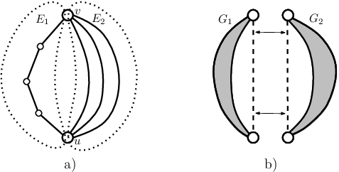
As described below, split-candidates make it possible to decompose completely a 2-connected graph into 3-connected components. We consider here only 2-connected graphs with at least three edges (graphs with less edges are degenerated for this decomposition). Given a split-candidate $S=\{E_{1},E_{2},u,v\}$ in a 2-connected graph $G$ (see Figure 6(b)), the corresponding split operation is defined as follows, see Figure 6(b):

•

an edge $e$ , called a virtual edge, is added between $u$ and $v$ ,
•

the graph $G[E_{1}]$ is separated from the graph $G[E_{2}]$ by cutting along the edge $e$ .

Such a split operation yields two graphs $G_{1}$ and $G_{2}$ , which correspond respectively to $G[E_{1}]$ and $G[E_{2}]$ , together with $e$ as a real edge; see Figure 6(b). The graphs $G_{1}$ and $G_{2}$ are said to be matched by the virtual edge $e$ . It is easily checked that $G_{1}$ and $G_{2}$ are 2-connected (and have at least three edges). The splitting process can be repeated until no split-candidate remains.

As shown by Tutte in [33], the structure resulting from the split operations is independent of the order in which they are performed. It is a collection of graphs, called the bricks of $G$ , which are articulated around virtual edges; see Figure 7(b). By definition of the decomposition, each brick has no split-candidate; Tutte shows that such graphs are either multiedge-graphs (M-bricks) or ring-graphs (R-bricks), or 3-connected graphs with at least four vertices (T-bricks).

The RMT-tree of $G$ is the graph $\tau(G)$ whose inner nodes correspond to the bricks of $G$ , and the edges between such vertices correspond to the virtual edges of $G$ (each virtual edge matches two bricks); additionally the leaves of $\tau(G)$ correspond to the real (not virtual) edges of $G$ ; see Figure 7. The graph $\tau(G)$ is indeed a tree [33]. By maximality of the decomposition, it is easily checked that $\tau(G)$ has no two adjacent R-bricks nor two adjacent M-bricks.

We will use the following inequalities to get a diameter estimate for random 2-connected planar graphs from a diameter estimate for random 3-connected planar graphs (which are equivalent to random $3$ -connected maps, by Whitney’s theorem). For a 2-connected planar graph $G$ , with RMT-tree $\tau$ , bricks $B_{1},\ldots,B_{k}$ , and $\mathcal{E}_{\mathrm{virt}}$ as the set of pairs of vertices of $G$ connected by a virtual edge, we have:

(8)

\displaystyle\mathrm{max}_{i}(\mathrm{diam}(B_{i}))\leq\mathrm{diam}(G)\leq\mathrm{max}_{i}(\mathrm{diam}(B_{i}))\cdot(\mathrm{diam}(\tau)+1)\cdot\mathrm{max}_{(u,v)\in\mathcal{E}_{\mathrm{virt}}}\mathrm{Dist}_{G}(u,v).

The first inequality is trivial. The second inequality follows from the following facts:

•

a diametral path $P_{G}$ in $G$ induces a path $P$ in $\tau$ (of length at most $\mathrm{diam}(\tau)$ ),
•

for each brick $B$ traversed by $P_{G}$ ( $B$ corresponds to a vertex of $\tau$ that lies on $P$ , there are $\mathrm{diam}(\tau)+1$ such vertices), the path $P_{G}$ induces a path $P_{B}=(v_{0},\ldots,v_{k})$ in $B$ , where each edge $\{v_{i},v_{i+1}\}$ is either a virtual edge or a real edge of $G$ .
•

the length of $P_{G}$ “used” when traversing an edge $e=\{v_{i},v_{i+1}\}\in P_{B}$ is at most the distance between $v_{i}$ and $v_{i+1}$ in $G$ .

Hence the length of $P_{G}$ “used by $B$ ” is at most $\mathrm{diam}(B)\cdot\mathrm{max}_{(u,v)\in\mathcal{E}_{\mathrm{virt}}}\mathrm{Dist}(u,v)$ , so that the total length of $P_{G}$ is given by the second inequality.

3. Diameter estimates for families of maps

In this section we consider families of maps, starting with quadrangulations and ending with $3$ -connected maps. In each case we show that for a random map $G$ of size $n$ in such a family, we have $\mathrm{diam}(G)\in(n^{1/4-\epsilon},n^{1/4+\epsilon})$ a.a.s. with exponential rate, where the size parameter $n$ is typically the number of edges or the number of faces. In order to carry later on (in Section 4) such estimates from 3-connected maps to connected planar graphs, we need to show that such concentration properties hold more generally in a weighted setting. More precisely, if a combinatorial class $\mathcal{G}=\cup_{n}\mathcal{G}_{n}$ (each $\gamma\in\mathcal{G}$ has a size $|\gamma|\in\mathbb{N}$ , and the set of objects of $\mathcal{G}$ of size $n$ is denoted $\mathcal{G}_{n}$ ) has an additional weight-function $w(\cdot)$ , then the generating function of $\mathcal{G}$ is

G(z)=\sum_{\alpha\in\mathcal{G}}w(\alpha)z^{|\alpha|},

and the weighted probability distribution in size $n$ assigns to each map $G\in\mathcal{G}_{n}$ the probability

\mathbb{P}(G)=\frac{w(G)}{C_{n}},\ \ \mathrm{with}\ C_{n}=\sum_{G\in\mathcal{G}_{n}}w(G).

Typically, for planar maps and planar graphs, the weight will be of the form $w(G)=x^{\chi(G)}$ , with $x$ a fixed positive real value and $\chi$ a parameter such as the number of vertices; in that case the terminology will be “a random map of size $n$ with weight $x$ at vertices”.

3.1. Quadrangulations

From Schaeffer’s bijection in Section 2.2.1 it is easy to show large deviation results for the diameter of a quadrangulation. The basic idea, originating in [10], is that the typical depth $k$ of a vertex in the tree is $n^{1/2}$ , and the typical discrepancy of the labels along a branch is $k^{1/2}=n^{1/4}$ . We use a fundamental result from [14], namely that under very general conditions the height of a random tree of size $n$ from a given family is in $(n^{1/2-\epsilon},n^{1/2+\epsilon})$ a.a.s. with exponential rate.

Let $y(z)=\sum_{\tau\in\mathcal{T}}z^{|\tau|}w(\tau)$ be the weighted generating function of some combinatorial class $\mathcal{T}$ (typically $\mathcal{T}$ is a class of rooted trees), and denote by $\rho$ the radius of convergence of $y(z)$ , assumed to be strictly positive. Assume $y\equiv y(z)$ satisfies an equation of the form

(9)

y=F(z,y),

with $F(z,y)$ a bivariate function with nonnegative coefficients, nonlinear in $y$ , analytic around $(0,0)$ , such that $F(0,0)=0$ and $F(0,y)=0$ . By the non-linearity of (9) with respect to $y$ , $y(\rho)$ is finite; let $\tau=y(\rho)$ . Equation (9) is called admissible if $F(z,y)$ is analytic at $(\rho,\tau)$ , in which case $F_{y}(\rho,\tau)=1$ . Equation (9) is called critical if $F(z,y)$ is not analytic at $(\rho,\tau)$ but $F(\rho,\tau)$ converges as a sum and $F(\rho,\tau)<1$ , which is equivalent to the fact that $y^{\prime}(z)$ converges at $\rho$ . A height-parameter for (9) is a nonnegative integer parameter $\xi$ for structures in $\mathcal{T}$ such that $y_{h}(z)=\sum_{\tau\in\mathcal{T},\xi(\tau)\leq h}w(\tau)z^{|\tau|}$ satisfies

y_{h+1}(z)=F(z,y_{h}(z))\ \ \mathrm{for}\ h\geq 0,\ \ \ y_{0}=0.

Lemma 3.1 (Theorem 1.3. in [14]).

Let $\mathcal{T}$ be a combinatorial class endowed with a weight-function $w(\cdot)$ so that the corresponding weighted generating function $y(z)$ satisfies an equation of the form (9), and such that (9) is admissible.

Let $\xi$ be a height-parameter for (9) and let $T_{n}$ be taken at random in $\mathcal{T}_{n}$ under the weighted distribution in size $n$ . Then $\xi(T_{n})\in(n^{1/2-\epsilon},n^{1/2+\epsilon})$ a.a.s. with exponential rate.

Remark 3.2.

Theorem 1.3 in [14] actually gives bounds for the coefficients $[z^{n}]y_{h}(z)$ from which Lemma 3.1 directly follows, observing that $P(\xi(T_{n})>h)=([z^{n}](y(z)-y_{h}(z)))/[z^{n}]y(z)$ and $P(\xi(T_{n})\leq h)=[z^{n}]y_{h}(z)/[z^{n}]y(z)$ . The authors of [14] prove the result for plane trees, then they claim that all the arguments in the proof hold for any system of the form $y=z\phi(y)$ . The arguments hold even more generally for any admissible system of the form $y=F(z,y)$ .

The next proposition is proved as a warm up, what we will need is a weighted version that is more technical to prove.

Proposition 3.3.

The diameter of a random rooted quadrangulation with $n$ faces is, a.a.s. with exponential rate, in the interval $(n^{1/4-\epsilon},n^{1/4+\epsilon})$ .

Proof.

When the number of black vertices is not taken into account, the statement of Theorem 2.2 simplifies: it gives a $1$ -to- $2$ correspondence between labelled trees having $n$ edges and rooted quadrangulations having $n$ faces and a secondary marked vertex; once again for a vertex $v$ of a labelled tree $\tau$ , the quantity $\ell_{v}-\ell_{\mathrm{min}}+1$ gives the distance of $v$ from the marked vertex in the associated quadrangulation. According to (3), we just have to show that, for a uniformly random labelled tree $\tau$ with $n$ vertices, $L(\tau)=\ell_{\mathrm{max}}-\ell_{\mathrm{min}}$ is in $(n^{1/4-\epsilon},n^{1/4+\epsilon})$ a.a.s. with exponential rate. Since the label either increases by $1$ , stays equal, or decreases by $1$ along each edge (going away from the root), the series $T(z)$ of labelled trees counted according to vertices satisfies

T(z)=\frac{z}{1-3T(z)},

and the usual height of the tree is a height-parameter for this equation. The equation is clearly admissible (the singularity is at $1/12$ and $T(1/12)=1/6$ ), hence by Lemma 3.1 the height is in $(n^{1/2-\epsilon},n^{1/2+\epsilon})$ a.a.s. with exponential rate. So in a random labelled tree there is a.a.s. with exponential rate a path $B$ of length $k=n^{1/2-\epsilon}$ starting from the root. The labels along $B$ form a random walk with increments $+1$ , $0$ , $-1$ , each with probability $1/3$ . Classically the maximum of such a walk is at least $k^{1/2-\epsilon}$ (which is at least $n^{1/4-\epsilon}$ ) a.a.s. with exponential rate. Hence the label of the vertex $v$ on $B$ at which the maximum occurs is at least the label of the root-vertex plus $n^{1/4-\epsilon}$ , so $\ell_{max}\geq n^{1/4-\epsilon}$ a.a.s. with exponential rate. Since $\ell_{min}\leq 0$ , this proves the lower bound.

For the upper bound (already proved in [10]), since the height is at most $n^{1/2+\epsilon}$ a.a.s. with exponential rate, the same is true for the depth $k$ of a random vertex $v$ in a random labelled tree of size $n$ . The labels along the path from the root to $v$ form a random walk of length $k$ , the maximum of which is at most $k^{1/2+\epsilon}$ a.a.s. with exponential rate. Hence $|\ell(v)|\leq n^{(1/2+\epsilon)^{2}}$ a.a.s. with exponential rate, so the same holds for the property $|\ell(v)|\leq n^{1/4+\epsilon}$ . Since multiplying by $n$ keeps the probability of failure exponentially small, the property $\{\forall v\in Q,\ |\ell(v)|\leq n^{1/4+\epsilon}\}$ is true a.a.s. with exponential rate. This completes the proof. ∎

The next theorem generalizes Proposition 3.3 to the weighted case, which is needed later on. The analytical part of the proof is more delicate since the system specifying weighted labelled trees needs two lines, and has to be transformed to a one-line equation in order to apply Lemma 3.1.

Theorem 3.4.

Let $0<a<b$ . The diameter of a random rooted quadrangulation with $n$ faces and weight $x$ at black vertices is, a.a.s. with exponential rate, in the interval $(n^{1/4-\epsilon},n^{1/4+\epsilon})$ , uniformly over $x\in[a,b]$ .

Proof.

A bicolored labelled tree is called black-rooted (resp. white-rooted) if the root-vertex is black (resp. white). In a bicolored labelled tree the white-black depth of a vertex $v$ is defined as the number of edges going from a white to a black vertex on the path from the root-vertex to $v$ , and the white-black height is defined as the maximum of the white-black depth over all vertices. We use here a decomposition of a bicolored labelled tree into monocolored components (the components are obtained by removing the bicolored edges), each such component being a plane tree. Let $f(z)$ (resp. $g(z)$ ) be the weighted generating function of black-rooted (resp. white-rooted) bicolored labelled trees, where $z$ marks the number of vertices, and where each tree $\tau$ with $i$ black vertices has weight $w(\tau)=x^{i}$ . Let $T(z)$ be the series counting rooted plane trees according to edges, $T(z)=1/(1-zT(z))$ . A tree counted by $f(z)$ is made of a monochromatic component (a rooted plane tree) where in each corner one might insert a sequence of trees counted by $g(z)$ ; in addition each time one inserts a tree counted by $g(z)$ one has to choose if the label increases or decreases along the corresponding black-white edge. Since a rooted plane tree with $k$ edges has $2k+1$ corners and $k+1$ vertices, we obtain

f(z)=\frac{xz}{1-2g(z)}T\left(\frac{xz}{(1-2g(z))^{2}}\right).

Similarly

g(z)=\frac{z}{1-2f(z)}T\left(\frac{z}{(1-2f(z))^{2}}\right).

Hence the series $y=f(z)$ satisfies the equation $y=F(z,y)$ , where $F(z,y)$ is expressed by

(10)

\begin{array}[]{ll}F(z,y)=\displaystyle\frac{xz}{1-2G(z,y)}T\left(\frac{xz}{(1-2G(z,y))^{2}}\right),\\ G(z,y)=\displaystyle\frac{z}{1-2y}T\left(\frac{z}{(1-2y)^{2}}\right).\end{array}

In addition, the white-black height is a height-parameter for this system.

Claim. The system (10) is admissible.

Proof of the claim. Let $\rho$ be the singularity of $f(z)$ and $\tau=f(\rho)$ . Let us prove first that $G(z,y)$ is analytic at $(\rho,\tau)$ . Note that $\tau<1/2$ , otherwise there would be $z_{0}\leq\rho$ such that $f(z_{0})=1/2$ , in which case $g(z)$ (and $f(z)$ as well) would diverge to $\infty$ as $z\to z_{0}^{-}$ , contradicting the fact that $f(z)$ converges for $0\leq|z|\leq\rho$ . The other possible cause of singularity is $\rho/(1-2\tau)^{2}$ being a singularity of $T(z)$ . We use the symbol $\succeq$ for coefficient-domination, i.e., $A(z)\succeq B(z)$ if $[z^{n}]A(z)\geq[z^{n}]B(z)$ for all $n\geq 0$ . Clearly we have

f(z)\succeq 2xzg(z),\ \ \ \ g^{\prime}(z)\succeq 2zf^{\prime}(z)T^{\prime}\left(\frac{z}{(1-2f(z))^{2}}\right),

hence

f^{\prime}(z)\succeq 4xz^{2}f^{\prime}(z)T^{\prime}\left(\frac{z}{(1-2f(z))^{2}}\right).

As a consequence,

T^{\prime}\left(\frac{z}{(1-2f(z))^{2}}\right)\leq\frac{1}{4xz^{2}},\quad\mathrm{as}\ z\to\rho^{-}.

Since $T^{\prime}(u)$ diverges at its singularity $1/4$ , we have $\rho/(1-2\tau)^{2}\neq 1/4$ , otherwise there would be the contradiction that the left-hand side diverges whereas the right-hand side, which is larger, converges as $z\to\rho^{-}$ . Hence $T$ is analytic at $\rho/(1-2\tau)^{2}$ , which ensures that $G(z,y)$ is analytic at $(\rho,\tau)$ . One proves similarly that $F(z,y)$ is also analytic at $(\rho,\tau)$ . $\triangle$

The claim, combined with Lemma 3.1, ensures that the white-black height of a random black-rooted bicolored labelled tree with $n$ edges and weight $x$ at black vertices ( $x\in[a,b]$ ) is in $(n^{1/2-\epsilon},n^{1/2+\epsilon})$ a.a.s. with exponential rate. In addition, the chain of calculations in [14] to prove Lemma 3.1 is easily seen to be uniform in $x\in[a,b]$ . A similar analysis ensures that the white-black height of a random white-rooted bicolored labelled tree with $n$ edges and weight $x$ at black vertices is in $(n^{1/2-\epsilon},n^{1/2+\epsilon})$ a.a.s. with exponential rate. Hence, overall, the white-black height of a random bicolored tree (either black-rooted or white-rooted) with $n$ edges and weight $x$ at black vertices is in $(n^{1/2-\epsilon},n^{1/2+\epsilon})$ a.a.s. with exponential rate.

Now the proof can be concluded in a similar way as in Proposition 3.3. Define the bicolored depth of a vertex $v$ from the root as the number of bicolored edges on the path from the root to $v$ , and define the bicolored height as the maximum of the bicolored depth over all vertices in the tree. Note that the bicolored depth $d(v)$ and the white-black depth $d^{\prime}(v)$ of a vertex $v$ satisfy the inequalities $2d^{\prime}(v)-1\leq d(v)\leq 2d^{\prime}(v)+1$ , so the bicolored height is in $(n^{1/2-\epsilon},n^{1/2+\epsilon})$ a.a.s. with exponential rate, uniformly over $x\in[a,b]$ . Similarly as in Proposition 3.3, this ensures that $\ell_{max}-\ell_{min}$ is in $(n^{1/4-\epsilon},n^{1/4+\epsilon})$ a.a.s. with exponential rate. And the uniformity over $x\in[a,b]$ follows from the uniformity over $x\in[a,b]$ for the height.

Finally, using the bijection of Theorem 2.2, the property that $\ell_{max}-\ell_{min}$ is in $(n^{1/4-\epsilon},n^{1/4+\epsilon})$ a.a.s. with exponential rate is transferred to the property that the diameter of a random quadrangulation with $n$ faces (with a marked vertex and a marked edge) and weight $x$ at each black vertex is in $(n^{1/4-\epsilon},n^{1/4+\epsilon})$ a.a.s. with exponential rate. There is however a last subtlety to deal with, namely that in the bijection from bicolored labelled trees to quadrangulations with a marked vertex and a marked edge, the number of black vertices in the tree corresponds either to the number of black vertices or to the number of black vertices plus one in the associated quadrangulation. So the weighted distribution (weight $x$ at black vertices) on bicolored labelled trees with $n$ edges is not exactly transported to the weighted distribution (weight $x$ at black vertices) on rooted quadrangulations with $n$ faces and a secondary marked vertex. However, since the inaccuracy on the number of black vertices in the quadrangulation is by at most one, the transported weighted distribution is biased by at most $x$ , so the large deviation result also holds under the (perfectly) weighted distribution for quadrangulations ¹¹ 1 The color of the marked vertex would be a delicate issue if we were trying to prove an explicit limit distribution (instead of large deviation results) for the diameter.. ∎

3.2. Maps

We use here the bijection of Section 2.2.2 to get a diameter estimate for random maps from a diameter estimate for random quadrangulations. First we need the following lemma.

Lemma 3.5.

Let $M(z,u)$ be the generating function of rooted maps, where $z$ marks the number of edges, $u$ marks the degree of the outer face, and with weight $x$ at each vertex. Let $\rho$ be the radius of convergence of $M(z,1)$ (note that $\rho$ depends on $x$ ). Then there is $u_{0}>1$ such that $M(\rho,u_{0})$ converges. In addition for $0<a<b$ , the value of $u_{0}$ can be chosen uniformly over $x\in[a,b]$ , and $M(\rho,u_{0})$ is uniformly bounded over $x\in[a,b]$ .

Proof.

The result follows easily from a bijection by Bouttier, Di Francesco and Guitter [7] between vertex-pointed planar maps and a certain family of decorated trees called mobiles, such that each face of degree $i$ in the map corresponds to a (black) vertex of degree $i$ in the mobile. Thanks to this bijection, the generating function $M^{\circ}(z,u)$ of rooted maps with a secondary marked vertex (where again $z$ marks the number of edges and $u$ marks the root-face degree) equals the generating function of rooted mobiles where $z$ marks half the total degree of (black) vertices and $u$ marks the root-vertex degree. Since mobiles (as rooted trees) satisfy an explicit decomposition at the root, the series $M^{\circ}(z,u)$ is easily shown to have, for any $x>0$ , a square-root singular development of the form

M^{\circ}(z,u)=a(z,u)-b(z,u)\sqrt{1-z/\rho},

valid in a neighborhood of $(\rho,1)$ , with $a(z,u)$ and $b(z,u)$ analytic in the parameters $z,u,x$ . Hence the statement holds for $M^{\circ}(z,u)$ . Since $M^{\circ}(z,u)$ dominates $M(z,u)$ coefficient-wise, the statement also holds for $M(z,u)$ . ∎

Theorem 3.6.

Let $0<a<b$ . The diameter of a random rooted map with $n$ edges and weight $x$ at the vertices is in the interval $(n^{1/4-\epsilon},n^{1/4+\epsilon})$ a.a.s. with exponential rate, uniformly over $x\in[a,b]$ .

Proof.

The first important observation is that the bijection of Section 2.2.2 transports the weighted (weight $x$ at black vertices) distribution on rooted quadrangulations with $n$ faces to the weighted (weight $x$ at vertices) distribution on rooted maps with $n$ edges. Let $M$ be a random rooted map with $n$ edges and let $Q$ be the associated rooted quadrangulation (with $n+2$ vertices). Since $\mathrm{diam}(Q)\leq 2\ \!\mathrm{diam}(M)$ , the diameter of $M$ is at least $n^{1/4-\epsilon}$ a.a.s. with exponential rate. The upper bound is proved from the inequality $\mathrm{diam}(M)\leq\mathrm{diam}(Q)\cdot\Delta(M)$ , where $\Delta(M)$ is the maximal face degree in $M$ . Together with Lemma 2.1, Lemma 3.5 ensures that the root-face degree $\delta(M)$ in a random rooted planar map with $n$ edges and weight $x$ at vertices has exponentially fast decaying tail. The probability distribution of $\delta(M)$ is the same if $M$ is bi-rooted (i.e., has two roots that are possibly equal, the root-face being the face incident to the primary root). When exchanging the secondary root with the primary root, the root-face can be seen as a face $f$ taken at random under the distribution $P(f)=\mathrm{deg}(f)/(2n)$ . Thus $\delta(M)$ is distributed as the degree of the (random) face $f$ . Hence

P(\delta(M)\geq k)\geq\frac{k}{2n}P(\Delta(M)\geq k),

so that $\Delta(M)\leq n^{\epsilon}$ a.a.s. with exponential rate. We conclude from (4) that the diameter of $M$ is at most $n^{1/4+\epsilon}$ a.a.s. with exponential rate. The uniformity in $x\in[a,b]$ follows from the uniformity in $x\in[a,b]$ in Theorem 3.4 and Lemma 3.5. ∎

3.3. 2-connected maps

Let $x>0$ . Denote by $M(z)$ (resp. $C(z)$ ) the weighted generating function of rooted connected (resp. 2-connected) maps according to edges and with weight $x$ at non-root vertices. Since a core with $n$ edges has $2n$ corners where to insert (possibly empty) rooted maps, this decomposition yields

(11)

M(z)=\sum_{n\geq 0}z^{n}\sum_{\tau\in\mathcal{C}_{n}}\big(1+M(z)\big)^{2n}=C(H(z)),\ \ \mathrm{where}\ H(z)=z(1+M(z))^{2}.

An important property of the core-decomposition is that it preserves the distribution with weight $x$ at vertices. Precisely, let $M$ be a random rooted map with $n$ edges and weight $x$ at vertices. Let $C$ be the core of $M$ and let $k$ be its size. Let $M_{1},\ldots,M_{2k}$ be the pieces of $M$ , and $n_{1},\ldots,n_{2k}$ their sizes. Then, conditioned to having size $k$ , $C$ is a random rooted 2-connected map with $k$ edges and weight $x$ at vertices; and conditioned to having size $n_{i}$ , the $i$ th piece $M_{i}$ is a random rooted map with $n_{i}$ edges and weight $x$ at vertices.

Lemma 3.7.

Let $0<a<b$ , and let $x\in[a,b]$ . Let $\rho$ be the radius of convergence of $z\mapsto M(z)$ ( $M(z)$ gives weight $x$ to vertices). Following [4], define

\alpha=\frac{H(\rho)}{\rho H^{\prime}(\rho)}.

Let $n\geq 0$ , and let $M$ be a random rooted map with $n$ edges and weight $x$ at vertices. Let $X_{n}=|C|$ be the size of the core of $M$ , and let $M_{1},\ldots,M_{2|C|}$ be the pieces of $M$ . Then

P\left(X_{n}=\lfloor\alpha n\rfloor,\ \mathrm{max}(|M_{i}|)\leq n^{3/4}\right)\sim P\left(X_{n}=\lfloor\alpha n\rfloor\right)=\Theta\left(n^{-2/3}\right)

uniformly over $x\in[a,b]$ .

Proof.

The statement $P(X_{n}=\lfloor\alpha n\rfloor)=\Theta(n^{-2/3})$ uniformly over $x\in[a,b]$ follows from [4]. So what we have to prove is that $P(X_{n}=\lfloor\alpha n\rfloor,\ \mathrm{max}(|M_{i}|)>n^{3/4})=o(n^{-2/3})$ uniformly over $x\in[a,b]$ .

Claim. Given a fixed $\delta>0$ , we have for $i>n^{2/3+\delta}$

P(X_{n}=\lfloor\alpha n\rfloor,\ \ |M_{1}|=i)=O(\exp(-n^{\delta/2})).

Proof of the claim. Let $a_{m}$ be the number of rooted maps and $c_{m}$ the number of rooted 2-connected maps with $m$ edges. It follows from the (algebraic) generating function expressions [32, 3] that these numbers have the asymptotic estimates $a_{m}\sim c\rho^{-m}m^{-5/2}$ , $c_{m}\sim c^{\prime}\sigma^{-m}m^{-5/2}$ . Equation (11) implies

P(X_{n}=k)=c_{k}\frac{[z^{n}]H(z)^{k}}{a_{n}}.

It is proved in [19, Theorem 1 (iii)-(b)], (and the bounds are easily checked to hold uniformly over $x\in[a,b]$ ) that for $k\geq\alpha n+n^{2/3+\delta}$ ,

(12)

[z^{n}]H(z)^{k}=O(\sigma^{k}\rho^{-n}\exp(-n^{\delta})).

Let $k_{0}=\lfloor\alpha n\rfloor$ and let $n^{2/3+\delta}<i\leq n-k_{0}$ . We have

	$\displaystyle P(X_{n}=k_{0},\ \|M_{1}\|=i)$	$\displaystyle=$	$\displaystyle c_{k_{0}}\frac{a_{i}[z^{n-i}]z^{k_{0}}(1+M(z))^{2k_{0}-1}}{a_{n}}$
		$\displaystyle\leq$	$\displaystyle c_{k_{0}}\frac{a_{i}[z^{n-i}]H(z)^{k_{0}}}{a_{n}}=O(n^{5/2}\sigma^{-k_{0}}\rho^{n-i}[z^{n-i}]H(z)^{k_{0}}).$

Since $\alpha n/(n-i)\geq\alpha(1+i/n)$ , we have $\alpha n\geq\alpha(n-i)+\alpha i(n-i)/n=\alpha(n-i)+\Omega(n^{2/3+\delta})=\alpha(n-i)+\Omega((n-i)^{2/3+\delta})$ . Hence $k_{0}=\alpha(n-i)+\Omega((n-i)^{2/3+\delta})$ , so (12) ensures that for any fixed $\delta^{\prime}<\delta$ ,

[z^{n-i}]H(z)^{k_{0}}=O(\sigma^{k_{0}}\rho^{-n+i}\exp(-(n-i)^{\delta^{\prime}})).

Hence, for $i>n^{2/3+\delta}$ , and for any fixed $\delta^{\prime\prime}<\delta^{\prime}$ ,

P(X_{n}=k_{0},\ |M_{1}|=i)=O(\exp(-(n-i)^{\delta^{\prime\prime}})),

so that $P(X_{n}=k_{0},\ |M_{1}|=i)=O(\exp(-n^{\delta/2}))$ . $\triangle$

The claim implies that $P(X_{n}=\lfloor\alpha n\rfloor,\ |M_{1}|>n^{2/3+\delta})=O(n\exp(-n^{\delta/2}))$ , and by symmetry the same estimate holds for each piece $M_{i}$ . As a consequence $P(X_{n}=\lfloor\alpha n\rfloor,\ \mathrm{max}(|M_{i}|)>n^{2/3+\delta})=O(n^{2}\exp(-n^{\delta/2}))=O(\exp(-n^{\delta/3}))$ . Hence

P(X_{n}=\lfloor\alpha n\rfloor,\ \mathrm{max}(|M_{i}|)\leq n^{2/3+\delta})\sim P(X_{n}=\lfloor\alpha n\rfloor)=\Theta(n^{-2/3}).

This concludes the proof, taking $\delta=3/4-2/3=1/12$ . ∎

In [4] the authors show that $n^{2/3}P(X_{n}=\lfloor\alpha n\rfloor)$ converges; they even prove that $(X_{n}-\alpha n)/n^{2/3}$ converges in law. Lemma 3.7 just makes sure that the asymptotic estimate of $P(X_{n}=\lfloor\alpha n\rfloor)$ is the same under the additional condition that all pieces are of size at most $n^{3/4}$ (more generally, under the condition that all pieces are of size at most $n^{2/3+\delta}$ , for any $\delta>0$ ). A closely related result proved in [19] is that, for any fixed $\delta>0$ , there is a.a.s. no piece of size larger than $n^{2/3+\delta}$ provided the core has size larger than $n^{2/3+\delta}$ .

Theorem 3.8.

For $0<a<b$ , the diameter of a random rooted 2-connected map with $n$ edges and weight $x$ at vertices is, a.a.s. with exponential rate, in the interval $(n^{1/4-\epsilon},n^{1/4+\epsilon})$ , uniformly over $x\in[a,b]$ .

Proof.

Let $M$ be a rooted map with $n$ edges and weight $x$ at vertices. Denote by $C$ the core of $M$ and by $(M_{i})_{i\in[1..2|C|]}$ the pieces of $M$ . Since the event $\{|C|=\lfloor\alpha n\rfloor\}$ has polynomially small probability (order $\Theta(n^{-2/3})$ , as shown in [4]), and since the event $\mathrm{diam}(M)\leq n^{1/4+\epsilon}$ holds a.a.s. with exponential rate, the event $\mathrm{diam}(M)\leq n^{1/4+\epsilon}$ , knowing that $|C|=\lfloor\alpha n\rfloor$ , also holds a.a.s. with exponential rate. Since $\mathrm{diam}(M)\geq\mathrm{diam}(C)$ , we conclude that for $C$ a random 2-connected map with $\lfloor\alpha n\rfloor$ edges and weight $x$ at vertices, $\mathrm{diam}(C)\leq n^{1/4+\epsilon}$ a.a.s. with exponential rate. Of course the same holds for $C$ a random rooted 2-connected map with $n$ edges and weight $x$ at vertices. This yields the a.a.s. upper bound on $\mathrm{diam}(C)$ .

To prove the lower bound, we use Lemma 3.7, which ensures that the event

\{|C|=\lfloor\alpha n\rfloor,\ \mathrm{max}(|M_{i}|)\leq n^{3/4}\}

occurs with polynomially small probability, precisely $\Theta(n^{-2/3})$ . We claim that, under the condition that $\mathrm{max}(|M_{i}|)\leq n^{3/4}$ , then $\mathrm{max}(\mathrm{diam}(M_{i}))\leq n^{1/5}$ a.a.s. (in $n$ ) with exponential rate. Indeed, consider a piece $M_{i}$ of size $n_{i}$ . When $n_{i}\leq n^{1/5}$ , $\mathrm{diam}(M_{i})\leq n^{1/5}$ trivially. Moreover, Theorem 3.6 implies that, for $\delta>0$ small enough, $P(\mathrm{diam}(M_{i})>n_{i}^{1/4+\delta})\leq\exp(-n_{i}^{c\delta})$ for some $c>0$ . Hence when $n^{1/5}\leq n_{i}\leq n^{3/4}$ , $P(\mathrm{diam}(M_{i})>n^{3/4(1/4+\delta)})\leq\exp(-n^{c\delta/5})$ , and we can take $\delta$ small enough so that $3/4(1/4+\delta)\leq 1/5$ . Hence, when $n_{i}\leq n^{3/4}$ , the event $\mathrm{diam}(M_{i})>n^{1/5}$ has exponentially small probability in $n$ (meaning, in $O(\exp(-n^{\alpha})$ for some $\alpha>0$ ), and the same holds for $\mathrm{max}(\mathrm{diam}(M_{i}))$ . Hence

\mathbb{P}(\{|C|=\lfloor\alpha n\rfloor,\ \mathrm{max}(\mathrm{diam}(M_{i}))\leq n^{1/5}\})\sim\mathbb{P}(\{|C|=\lfloor\alpha n\rfloor\})=\Theta(n^{-2/3}).

In other words the event $\{|C|=\lfloor\alpha n\rfloor,\ \mathrm{max}(\mathrm{diam}(M_{i})\leq n^{1/5}\}$ occurs with polynomially small probability. In that case, since $\mathrm{diam}(C)\geq\mathrm{diam}(M)-2\ \!\mathrm{max}(\mathrm{diam}(M_{i}))$ , and since the event $\mathrm{diam}(M)<n^{1/4-\epsilon}$ occurs a.a.s. with exponential rate, we conclude that $\mathrm{diam}(C)\geq n^{1/4-\epsilon}-2n^{1/5}$ holds a.a.s. with exponential rate under the event $\mathcal{E}=\{|C|=\lfloor\alpha n\rfloor,\ \mathrm{max}(\mathrm{diam}(M_{i})\leq n^{1/5}\}$ . Since $\mathcal{E}$ occurs with probability $\Theta(n^{-2/3})$ and since $n^{1/5}=o(n^{1/4-\epsilon})$ for $\epsilon$ small enough, we conclude (similarly as in the proof of Theorem 3.8) that for $C$ a random 2-connected map with $\lfloor\alpha n\rfloor$ edges and weight $x$ at vertices, we have $\mathrm{diam}(C)\geq n^{1/4-\epsilon}$ a.a.s. with exponential rate. The same holds for $C$ a random rooted 2-connected with $n$ edges and weight $x$ at vertices.

The uniformity in $x\in[a,b]$ of the bounds follows from the uniformity in $x$ in Theorem 3.6 and Lemma 3.7. ∎

3.4. 3-connected maps

In the following we assume 3-connected maps (and 3-connected planar graphs) to have at least $4$ vertices, so the smallest 3-connected planar graph is $K_{4}$ . We use here the plane network decomposition (Section 2.2.4) to carry the diameter concentration property from 2-connected to 3-connected maps. For $x>0$ , call $N(z)$ (resp. $\widehat{N}(z)$ ) the weighted generating functions —weight $x$ at vertices not incident to the root-edge— of plane networks (resp. plane networks with a 3-connected core), where $z$ marks the number of edges. Note that $N(z)$ is very close to the generating function $C(z)$ of rooted 2-connected maps with weight $x$ at non-root vertices and with $z$ marking the number of edges:

C(z)=z+xz+xzN(z),

where the first two terms in the right-hand side stand for the two 2-connected maps with a single edge, either a loop or a link between two distinct vertices. Call $T(z)$ the weighted generating function of rooted 3-connected maps, with weight $x$ at vertices not incident to the root-edge, and with $z$ marking the number of non-root edges. Clearly, the weighted generating function $S(z)$ of plane networks decomposable as a sequence of plane networks satisfies $S(z)=(N(z)-S(z))xN(z)$ , hence $S(z)=xN(z)^{2}/(1+xN(z))$ . Similarly the weighted generating function $P(z)$ of parallel plane networks satisfies $P(z)=(N(z)-P(z))N(z)$ , so that $P(z)=N(z)^{2}/(1+N(z))$ . Hence

(13)

N(z)=S(z)+P(z)+\widehat{N}(z),

where

S(z)=\frac{xN(z)^{2}}{1+xN(z)},\quad P(z)=\frac{N(z)^{2}}{1+N(z)},\quad\widehat{N}(z)=T(N(z)).

An important remark is that a random plane network $C$ with $n$ edges and weight $x$ at vertices can be seen as a random $2$ -connected map with $n+1$ edges, weight $x$ at vertices, and where the root-edge has been deleted. Similarly as in Section 3.3, for a random plane network $N$ with $n$ edges and weight $x$ at vertices, and conditioned to have a 3-connected core $T$ of size $k$ , $T$ is a random rooted 3-connected map with $k$ edges and weight $x$ at vertices; and each piece $C_{e}$ conditioned to have a given size $n_{e}$ is a random plane network with $n_{e}$ edges and weight $x$ at vertices.

For proving the diameter estimate for 3-connected maps, we need the following lemma, ensuring that the root-face degree of a random 2-connected map is small.

Lemma 3.9.

Let $C(z,u)=\sum_{n,k}c_{n,k}z^{n}u^{k}$ be the generating function of rooted 2-connected maps, where $z$ marks the number of edges, $u$ marks the root-face degree, and with weight $x$ at each non-root vertex. Let $R$ be the radius of convergence of $C(z,1)$ . Then there is $v_{0}>1$ such that $C(\rho,v_{0})$ converges. In addition for $0<a<b$ , the value of $v_{0}$ can be chosen uniformly over $x\in[a,b]$ , and $C(z,v_{0})$ is uniformly bounded over $x\in[a,b]$ .

Proof.

The result has been established for arbitrary rooted maps in Lemma 3.5. To prove the result for 2-connected maps, we rewrite Equation (11) taking account of the root-face degree. Recall that a rooted map $\gamma$ is obtained from a rooted 2-connected map $\kappa$ where a rooted map (allowing for the one-vertex map) is inserted in each corner; call $k$ the root-face degree of $\kappa$ and $\gamma_{1},\ldots,\gamma_{k}$ the maps inserted in the root-face corners of $\kappa$ . If $d(M)$ denotes the root-face degree of a rooted map $M$ , then clearly

d(\gamma)=k+d(\gamma_{1})+\cdots+d(\gamma_{k}).

Hence, (with $M(z):=M(z,1)$ ):

M(z,u)=\sum_{n,k}c_{n,k}u^{k}(1+M(z))^{2n-k}(1+M(z,u))^{k},

so that

M(z,u)=C\left(z(1+M(z))^{2},u{1+M(z,u)\over 1+M(z)}\right).

Since the composition scheme is “critical” [4], it is known that, if $\rho$ denotes the radius of convergence of $M(z,1)$ , then $R=\rho\cdot(1+M(\rho))^{2}$ is the radius of convergence of $C(z,1)$ . Hence, since $M(\rho,u_{0})$ converges, $C(R,v_{0})$ converges for $v_{0}=u_{0}(1+M(\rho,u_{0}))/(1+M(\rho))>1$ . The uniformity statement for $C(z,u)$ (for $x\in[a,b]$ ) follows from the uniformity statement for $M(z,u)$ , established in Lemma 3.5, and the fact that $v_{0}$ is uniformly bounded away from $1$ when $x$ lies in a compact interval. ∎

Theorem 3.10.

Let $0<a<b$ . The diameter of a random 3-connected map with $n$ edges with weight $x$ at vertices is, a.a.s. with exponential rate, in the interval $(n^{1/4-\epsilon},n^{1/4+\epsilon})$ , uniformly over $x\in[a,b]$ .

Proof.

Let $\rho$ be the radius of convergence (depending on the weight $x$ at vertices) of $N(z)$ , which is the same as the radius of convergence of $C(z)=z+xz+xzN(z)$ . And let

\alpha=\frac{N(\rho)}{\rho N^{\prime}(\rho)}.

Again the results in [4] ensure that, for a random plane network $C$ with $n$ edges and weight $x$ at vertices, the probability of having a 3-connected core $T$ of size $\lfloor\alpha n\rfloor$ is $\Theta(n^{-2/3})$ , hence polynomially small, whereas the probability that $\mathrm{diam}(C)>n^{1/4+\epsilon}$ is exponentially small. Since $\mathrm{diam}(C)\geq\mathrm{diam}(T)$ , and since $T$ is a random rooted $3$ -connected map with $k=\lfloor\alpha n\rfloor$ edges and weight $x$ at vertices, we conclude that $\mathrm{diam}(T)\leq n^{1/4+\epsilon}$ a.a.s. with exponential rate. For the lower bound we look at the second inequality in (6):

\mathrm{diam}(C)\leq\mathrm{diam}(T)\cdot\mathrm{max}_{e\in T}(d_{e})+2\ \!\mathrm{max}_{e\in T}(\mathrm{diam}(C_{e})),

where for each edge $e$ of $T$ , $C_{e}$ denotes the piece substituted at $e$ and $d_{e}$ denotes the root-face degree of $C_{e}$ .

Lemma 2.1 and Lemma 3.9 ensure that the distribution of the root-face degree of a random rooted 2-connected map has exponentially fast decaying tail. Hence $\mathrm{max}_{e\in T}(d_{e})\leq n^{\epsilon}$ a.a.s. with exponential rate. Moreover, in the same way as in Lemma 3.7, one can show that the probability of the event $\mathcal{E}=\{|T|=\lfloor\alpha n\rfloor,\ \mathrm{max}(|C_{e}|)\leq n^{3/4}\}$ is $\Theta(n^{-2/3})$ . Since $\mathrm{max}_{e\in T}(d_{e})\leq n^{\epsilon}$ and $\mathrm{diam}(C)\geq n^{1/4-\epsilon}$ a.a.s. with exponential rate, Equation (6) easily implies that, conditioned on $\mathcal{E}$ , $\mathrm{diam}(T)\geq n^{1/4-\epsilon}$ a.a.s. with exponential rate. Since $\mathcal{E}$ occurs with polynomially small probability, we conclude that $\mathrm{diam}(T)\geq n^{1/4-\epsilon}$ a.a.s. with exponential rate. Finally the uniformity of the estimate over $x\in[a,b]$ follows from the uniformity over $x\in[a,b]$ in Theorem 3.8 and in Lemma 3.9. ∎

4. Diameter estimates for families of graphs

We now establish estimates (all of the form $\mathrm{diam}(G)\in(n^{1/4-\epsilon},n^{1/4+\epsilon})$ a.a.s. with exponential rate) for the diameter of random graphs in families of unembedded planar graphs. We establish first an estimate for 3-connected planar graphs (equivalent to 3-connected maps by Whitney’s theorem), then derive from it an estimate for 2-connected planar graphs (which have a decomposition, at edges, into 3-connected components), and finally derive from it an estimate for connected planar graphs (which have a decomposition, at vertices, into 2-connected components). Since the graphs are unembedded, it is necessary to label them to avoid symmetry issues (in contract, for maps, rooting, i.e., marking and orienting an edge, is enough). One can choose to label either the vertices or the edges. For our purpose it is more convenient to label 3-connected and 2-connected planar graphs at edges (because the decomposition into 3-connected components occurs at edges); then relabel 2-connected planar graphs at vertices and label also connected planar graphs at vertices (because the decomposition into 2-connected components occurs at vertices).

4.1. 3-connected planar graphs

For the time being we need 3-connected graphs labelled at the edges (this is enough to avoid symmetries). The number of edges is denoted $m$ , and $n$ is reserved for the number of vertices. By Whitney’s theorem, 3-connected planar graphs with at least $4$ vertices have two embeddings on the oriented sphere (which are mirror of each other). Hence Theorem 3.10 gives:

Theorem 4.1.

Let $0<a<b$ . The diameter of a random 3-connected planar graph with $m$ edges and weight $x$ at vertices is, a.a.s. with exponential rate, in the interval $(m^{1/4-\epsilon},m^{1/4+\epsilon})$ , uniformly over $x\in[a,b]$ .

4.2. Planar networks

Before handling 2-connected planar graphs we treat the closely related family of planar networks. A planar network is a connected simple planar graph with two marked vertices called the poles, such that adding an edge between the poles, called the root-edge, makes the graph 2-connected. First it is convenient to consider planar networks as labelled at the edges.

Theorem 4.2.

Let $0<a<b$ . The diameter of a random planar network with $m$ labelled edges and weight $x$ at vertices is, a.a.s. with exponential rate, in the interval

(m^{1/4-\epsilon},m^{1/4+\epsilon}),

uniformly over $x\in[a,b]$ .

The proof, which is quite technical, is delayed to Section 5; it relies on the decomposition into $3$ -connected components described in Section 2.3.2 and the inequalities (8). The proof of Theorem 4.9 in the next section, which relies on the decomposition into 2-connected components gives a good idea (with less technical details), of the different steps needed to prove Theorem 4.2.

Lemma 4.3.

Let $1<c<d<3$ . Let $N_{n,m}$ be a planar network with $n$ vertices and $m$ labelled edges, taken uniformly at random. Then $\mathrm{diam}(N_{n,m})\in(n^{1/4-\epsilon},n^{1/4+\epsilon})$ a.a.s. with exponential rate, uniformly over $m/n\in[c,d]$ .

Proof.

Let $\mu=m/n$ . For $x>0$ , let $X_{m}$ be the number of vertices of a random planar network $N$ with $m$ edges and weight $x$ at vertices. The results in [5] ensure that there exists $x_{\mu}>0$ such that, for $x=x_{\mu}$ , $P(X_{m}=n)=\Theta(m^{-1/2})$ , uniformly over $\mu\in[c,d]$ . In addition $x_{\mu}$ is a continuous function of $\mu$ , so it maps $[c,d]$ into a compact interval. Therefore, Theorem 4.2 implies that, for $x=x_{\mu}$ , $\mathrm{diam}(N)\in[m^{1/4-\epsilon},m^{1/4+\epsilon}]$ a.a.s. with exponential rate uniformly over $\mu\in[c,d]$ . Since $P(X_{m}=n)=\Theta(m^{-1/2})$ , uniformly over $\mu\in[c,d]$ , we conclude that the event $\mathrm{diam}(N)\in[m^{1/4-\epsilon},m^{1/4+\epsilon}]$ , conditioned on $X_{m}=n$ , holds a.a.s. with exponential rate uniformly over $\mu\in[c,d]$ , which concludes the proof (note that the distribution of $N$ conditioned on $X_{m}=n$ is the uniform distribution on planar networks with $m$ edges and $n$ vertices). ∎

The proof of Lemma 4.3 is the only place where uniformity of the estimates according to $x$ (for $x$ in an arbitrary compact interval) is needed. In the following, the weight $x$ will be at edges, and we will not need anymore to check that the statements hold uniformly in $x$ (even though they clearly do). Another important remark is that planar networks with $n$ vertices and $m$ edges can be labelled either at vertices or at edges, and the uniform distribution in one case corresponds to the uniform distribution in the second case. Hence the result of Lemma 4.3 holds for random planar networks with $n$ labelled vertices and $m$ unlabelled edges.

Lemma 4.4.

Let $x>0$ . Let $N$ be a random planar network with $n$ labelled vertices and weight $x$ at edges (which are unlabelled). Then $\mathrm{diam}(N)\in(n^{1/4-\epsilon},n^{1/4+\epsilon})$ a.a.s. with exponential rate.

Proof.

As shown in [5], the ratio $r=\#(edges)/\#(vertices)$ of $N$ is concentrated around some value $\mu=\mu(x)\in(1,3)$ . Precisely, for each $\delta>0$ , there is $c=c(\delta)>0$ such that

\mathbb{P}\{r\notin(\mu-\delta,\mu+\delta)\}\leq\exp(-cn).

Take $\delta$ small enough so that $r-\delta>1$ and $r+\delta<3$ . Then Lemma 4.3 ensures that $\mathrm{diam}(N)\in[n^{1/4-\epsilon},n^{1/4+\epsilon}]$ a.a.s. with exponential rate. ∎

4.3. 2-connected planar graphs

Planar networks are very closely related to edge-rooted $2$ -connected planar graphs. In fact, an edge-rooted (i.e., with a marked oriented edge) $2$ -connected planar graph $G$ yields two planar networks: one where the marked edge is kept (otherly stated, doubled and then one copy of the marked edge is deleted) and one where the marked edge is deleted (in the second case the diameter of the planar network might be larger than the diameter of $G$ , however by a factor of at most $2$ ). Consequently the statement of Lemma 4.4 also holds for $N$ a random edge-rooted $2$ -connected planar graph with $n$ (labelled) vertices and weight $x$ at edges. And the statement still holds for a random $2$ -connected planar graph (unrooted) with $n$ vertices, since the number of edges can vary only from $n$ to $3n$ (hence the effect of unmarking a root-edge biases the distribution by a factor of at most $3$ ). We obtain:

Theorem 4.5.

Let $x>0$ . The diameter of a random 2-connected planar graph with $n$ vertices and weight $x$ at edges is, a.a.s. with exponential rate, in the interval $(n^{1/4-\epsilon},n^{1/4+\epsilon})$ .

4.4. Connected planar graphs

Here we deduce from Theorem 4.5 that a random connected planar graph with $n$ vertices has diameter in $(n^{1/4-\epsilon},n^{1/4+\epsilon})$ a.a.s. with exponential rate. We use the block decomposition presented in Section 2.3.1, and the inequality (7). Again an important point is that if $C$ is a random connected planar graph with $n$ vertices and weight $x$ at edges, then each block $B$ of size $k$ in $C$ is a random $2$ -connected planar graph with $k$ vertices and weight $x$ at edges. Note that, formulated on pointed graphs (i.e., graphs with a marked vertex), the block-decomposition ensures that a pointed connected planar graph is obtained as follows: take a collection of 2-connected pointed planar graphs, and merge their marked vertices into a single vertex; then attach at each non-marked vertex $v$ in these blocks a pointed connected planar graph $C_{v}$ . Fix $x>0$ . Call $C(z)$ and $B(z)$ the weighted generating functions, respectively, of connected and 2-connected planar graphs with weight $x$ at edges. Then the decomposition above yields

(14)

C^{\prime}(z)=\exp(B^{\prime}(zC^{\prime}(z))).

Lemma 4.6.

For $x>0$ , a random connected planar graph with $n$ vertices and weight $x$ at edges has a block of size at least $n^{1-\epsilon}$ a.a.s. with exponential rate.

Proof.

Denote by $E(z)=zC^{\prime}(z)$ the series counting pointed connected planar graphs with weight $x$ at edges. Note that the functional inverse of $E(z)$ is $\phi(u)=u\exp(-g(u))$ , where $g(u)=B^{\prime}(u)$ . Call $\rho$ the radius of convergence of $C(z)$ and $R$ the radius of convergence of $B(u)$ . Define $b_{i}:=[u^{i}]g(u)$ , $g_{k}(u):=\sum_{i\leq k}b_{i}u^{i}$ , and call $E_{k}(z)$ the series of pointed connected planar graphs where all blocks have size at most $k$ . Note that the probability of a random connected planar graph with $n$ vertices to have all its blocks of size at most $k$ is $[z^{n}]E_{k}(z)/[z^{n}]E(z)$ . Clearly

E_{k}(z)=z\exp(g_{k}(E_{k}(z)),

hence the functional inverse of $E_{k}(z)$ is $\phi_{k}(u)=u\exp(-g_{k}(u))$ . Call $\rho_{k}$ the singularity of $E_{k}(z)$ . Since $\phi_{k}(u)$ is analytic everywhere, the singularity at $\rho_{k}$ is caused by a branch point, i.e., $\rho_{k}=\phi_{k}(R_{k})$ , where $R_{k}$ is the unique $u>0$ such that $\phi_{k}^{\prime}(u)=0$ : $\phi_{k}^{\prime}(u)>0$ for $0<u<R_{k}$ and $\phi^{\prime}(u)<0$ for $u>R_{k}$ . According to (2), $[z^{n}]E_{k}(z)\leq E_{k}(s)s^{-n}$ for $s<\rho_{k}$ , or equivalently, writing $u=E_{k}(s)$ ,

(15)

[z^{n}]E_{k}(z)\leq u\phi_{k}(u)^{-n}\ \ \mathrm{for\ all}\ u\ \mathrm{such\ that}\ \phi_{k}^{\prime}(u)>0.

Define $u_{k}=R\cdot(1+1/(k\log k))$ . Note that

g_{k}(R)\leq g_{k}(u_{k})\leq\left(\frac{u_{k}}{R}\right)^{k}g_{k}(R).

Since $(u_{k}/R)^{k}\to 1$ we have $g_{k}(u_{k})\to g(R)$ . Similarly $g_{k}^{\prime}(u_{k})\to g^{\prime}(R)$ , hence $\phi_{k}^{\prime}(u_{k})\to\phi^{\prime}(R)$ . It is shown in [20] that $a=\phi^{\prime}(R)$ is strictly positive (i.e., the singularity of $E(z)$ is not due to a branch point), so for $k$ large enough, $\phi_{k}^{\prime}(u_{k})\geq a/2>0$ , i.e., the bound (15) can be used, giving

[z^{n}]E_{k}(z)\leq 2\ \!R\ \!\phi_{k}(u_{k})^{-n}\ \ \mathrm{for\ }k\ \mathrm{large\ enough\ and\ any}\ n\geq 0.

Moreover

\phi_{k}(u_{k})-\rho=\left(\phi_{k}(u_{k})-\phi_{k}(R)\right)+\left(\phi_{k}(R)-\phi(R)\right)=a\cdot(u_{k}-R)+O(k^{-3/2})\sim\frac{a\ \!R}{k\log k},

where $\phi_{k}(R)-\phi(R)=O(k^{-3/2})$ is due to $g(R)-g_{k}(R)=O(k^{-3/2})$ , which itself follows from the estimate $b_{i}=\Theta(R^{-i}i^{-5/2})$ shown in [20]. Hence for $k$ large enough and any $n\geq 0$ :

[z^{n}]E_{k}(z)\leq 2\left(\rho+\frac{a\ \!R}{2k\log k}\right)^{-n}.

Hence, for $k=n^{1-\epsilon}$ , $[z^{n}]E_{k}(z)=O(\rho^{-n}\exp(-n^{\epsilon/2}))$ . Finally, according to [20], $[z^{n}]E(z)=\Theta(\rho^{-n}n^{-5/2})$ , so $[z^{n}]E_{k}(z)/[z^{n}]E(z)=O(\exp(-n^{\epsilon/3}))$ . ∎

Remark.

It is shown in [22] and [30] that a random connected planar graph has a.a.s. a block of linear size, but not with exponential rate. This is the reason for the previous lemma.

Lemma 4.6 directly implies that a random connected planar graph with $n$ vertices has diameter at least $n^{1/4-\epsilon}$ . Indeed it has a block of size $k\geq n^{1-\epsilon}$ a.a.s. with exponential rate and since the block is uniformly distributed in size $k$ , it has diameter at least $k^{1/4-\epsilon}$ a.a.s. with exponential rate.

Let us now prove the upper bound. For this purpose we use the inequality given in Section 2.3.1:

\mathrm{diam}(C)\leq(\mathrm{diam}(\tau)+1)\cdot\mathrm{max}_{i}(\mathrm{diam}(B_{i})),

where $C$ denotes a connected planar graph, $\tau$ is the Bv-tree, and the $B_{i}$ ’s are the blocks of $C$ . We show that $\mathrm{diam}(\tau)\leq n^{\epsilon}$ a.a.s. and that $\mathrm{max}_{i}(\mathrm{diam}(B_{i}))\leq n^{1/4+\epsilon}$ a.a.s., both with exponential rate.

To show that $\mathrm{diam}(\tau)\leq n^{\epsilon}$ we need a counterpart of Lemma 3.1 for critical equations of the form (9) (Indeed, note that $y\equiv y(z)=C^{\prime}(z)$ is solution of $y=F(z,y)$ , where $F(z,y)=\exp(B^{\prime}(zy))$ ; in addition the height of the Bv-tree, rooted at the pointed vertex, is a height-parameter of that system.)

Lemma 4.7.

Let $\mathcal{T}$ be a combinatorial class endowed with a weight-function $w(\cdot)$ so that the corresponding (weighted) generating function $y(z)$ satisfies an equation of the form $y=F(z,y)$ that is critical.

Let $\xi$ be a height-parameter for (9) and let $T_{n}$ be taken at random in $\mathcal{T}_{n}$ under the weighted distribution in size $n$ . Assume that $[z^{n}]y(z)=\Omega(n^{-\alpha}\rho^{-n})$ for some $\alpha$ . Then $\xi(T_{n})\leq n^{\epsilon}$ a.a.s. with exponential rate.

Proof.

For $h\geq 0$ we define the generating function $y_{h}(z)=\sum_{\tau\in\mathcal{T},\ \xi(\tau)\leq h}z^{|\tau|}w(\tau)$ , so that

y_{h}(z)=F(z,y_{h-1}(z)),

and define $\overline{y}_{h}(z)=\sum_{\tau\in\mathcal{T},\ \xi(\tau)=h}z^{|\tau|}w(\tau)$ (i.e., $\overline{y}_{h}(z)=y_{h}(z)-y_{h-1}(z)$ ). Let $\tau_{h}=y_{h}(\rho)$ and $\overline{\tau}_{h}=\overline{y}_{h}(\rho)$ . Note that $y(z,u)=\sum_{h}\overline{y}_{h}(z)u^{h}$ is the bivariate generating function of $\mathcal{T}$ where $z$ marks the size and $u$ marks the height. For $h>0$ we have

\tau_{h+1}-\tau_{h}=F(\rho,\tau_{h})-F(\rho,\tau_{h-1})=F_{y}(\rho,u_{h})\cdot(\tau_{h}-\tau_{h-1}),\ \ \mathrm{for\ some\ }u_{h}\in[\tau_{h-1},\tau_{h}].

Since $\tau_{h}$ converges to $\tau$ as $h\to\infty$ , $u_{h}$ also converges to $\tau$ , hence $F_{y}(\rho,u_{h})$ converges to $F_{y}(\rho,\tau)<1$ . Consequently $\overline{\tau}_{h}=\tau_{h}-\tau_{h-1}$ is $O(\exp(-ch))$ for some $c>0$ , so that $y(\rho,u)$ converges for $u<\exp(c)$ . Hence, by Lemma 2.1, we conclude that $\xi(T_{n})\leq n^{\epsilon}$ a.a.s. with exponential rate. ∎

Lemma 4.8.

For $x>0$ , the block-decomposition tree $\tau$ of a random connected planar graph with $n$ vertices and weight $x$ at edges has diameter at most $n^{\epsilon}$ a.a.s. with exponential rate.

Proof.

Let $C$ be a pointed connected planar graph, and $\tau$ the associated Bv-tree, rooted at the marked vertex of $C$ . Define the block-height $h(\tau)$ of $\tau$ as the maximal number of blocks (B-nodes) over all paths starting from the root. Clearly $\mathrm{diam}(\tau)\leq 4h(\tau)+4$ . In addition the block-height is clearly a height-parameter for the equation

y=F(z,y),\ \ \ \mathrm{where}\ F(z,y)=z\exp(B^{\prime}(y))

satisfied by the (weighted) generating function $y(z)=zC^{\prime}(z)$ of pointed connected planar graphs. It is shown in [20] that $y^{\prime}(z)$ converges at its radius of convergence $\rho$ . Hence the equation is critical; by Lemma 4.7, $h(\tau)\leq n^{\epsilon}$ a.a.s. with exponential rate, hence $\mathrm{diam}(\tau)\leq n^{\epsilon}$ a.a.s. with exponential rate. ∎

Lemma 4.8 easily implies that the diameter of a random connected planar graph $C$ with $n$ vertices is at most $n^{1/4+\epsilon}$ a.a.s. with exponential rate. Indeed, calling $\tau$ the block-decomposition tree of $C$ and $B_{i}$ the blocks of $C$ , one has

\mathrm{diam}(C)\leq(\mathrm{diam}(\tau)+1)\cdot\mathrm{max}_{i}(\mathrm{diam}(B_{i})).

Lemma 4.8 ensures that $\mathrm{diam}(\tau)\leq n^{\epsilon}$ a.a.s. with exponential rate. Moreover Theorem 4.5 easily implies that a random 2-connected planar graph of size $k\leq n$ has diameter at most $n^{1/4+\epsilon}$ a.a.s. with exponential rate, whatever $k\leq n$ is (proof by splitting in two cases: $k\leq n^{1/4}$ and $n^{1/4}\leq k\leq n$ , similarly as in the proof of Theorem 3.8). Hence, since each of the blocks has size at most $n$ , $\mathrm{max}_{i}(\mathrm{diam}(B_{i}))\leq n^{1/4+\epsilon}$ a.a.s. with exponential rate. Therefore we have

Theorem 4.9.

For $x>0$ , the diameter of a random connected planar graph with $n$ vertices and weight $x$ at edges is, a.a.s. with exponential rate, in the interval $(n^{1/4-\epsilon},n^{1/4+\epsilon})$ .

We can now complete the proof of Theorems 1.1 and 1.2. Theorem 1.1 is just Theorem 4.9 for $x=1$ . To show Theorem 1.2, one uses the fact (proved in [20]) that for each $\mu\in(1,3)$ there exists $x>0$ such that a random connected planar graph with $n$ edges and weight $x$ at edges has probability $\Theta(n^{-1/2})$ to have $\lfloor\mu n\rfloor$ edges.

5. Proof of Theorem 4.2

The proof of Theorem 4.2 follows the same lines as the proof of Theorem 4.9, with the RMT-tree playing the role that the Bv-tree had in Theorem 4.9. The lower bound is obtained from the fact, established in Lemma 5.2, that a random planar network has a.a.s. a “big” 3-connected component. The upper bound is obtained from the inequality given in Section 2.3.2,

(16)

\mathrm{diam}(G)\leq\mathrm{max}_{i}(\mathrm{diam}(B_{i}))\cdot(\mathrm{diam}(\tau)+1)\cdot\mathrm{max}_{(u,v)\in\mathcal{E}_{\mathrm{virt}}}\mathrm{Dist}_{G}(u,v)

where $G$ is the 2-connected planar graph obtained by connecting the two poles of the considered planar network, $\tau$ is the RMT-tree of $G$ , the $B_{i}$ ’s are the bricks of $G$ , and $\mathcal{E}_{\mathrm{virt}}$ is the set of virtual edges of $G$ . To get the upper bound we will successively prove that a.a.s. with exponential rate we have $\mathrm{diam}(\tau)\leq m^{\epsilon}$ (in Lemma 5.4), $\mathrm{max}_{i}(\mathrm{diam}(B_{i}))\leq m^{1/4+\epsilon}$ (in Lemma 5.5), and $\mathrm{max}_{(u,v)\in\mathcal{E}_{\mathrm{virt}}}\mathrm{Dist}_{G}(u,v)\leq m^{\epsilon}$ (in Lemma 5.8).

First we need the following lemma, which is a counterpart of Lemmas 3.5 and 3.9 for 3-connected maps.

Lemma 5.1.

Let $T(z,u)$ be the generating function of rooted $3$ -connected maps where $z$ marks the number of non-root edges, $u$ marks the root-face degree, and with weight $x$ at each vertex not incident to the root-edge. Let $\rho$ be the radius of convergence of $T(z,1)$ . Then there is $u_{0}>1$ such that $T(\rho,u_{0})$ converges. In addition for $0<a<b$ , the value of $u_{0}$ can be chosen uniformly over $x\in[a,b]$ , and $M_{i}(z,u_{0})$ is uniformly bounded over $x\in[a,b]$ .

Proof.

The result is derived from Lemma 3.9 using a bivariate version of Equation (13), in the very same way that Lemma 3.9 is derived from Lemma 3.5 using a bivariate version of Equation (11). ∎

To carry out the proof it is useful to rely on a well-known recursive decomposition of planar networks that derives from the RMT-tree. Call a planar network $D$ polyhedral if the poles are not adjacent and the addition of an edge between the poles gives a $3$ -connected planar graph with at least $4$ vertices. Similarly as in the case of embedded graphs (see Section 2.2.4), a planar network is either obtained as several planar networks in series (S-network), or as several planar networks in parallel (P-network), or as a polyhedral planar network where each edge is substituted by an arbitrary planar network (H-network). This can also be seen using the RMT-tree. Indeed let $B=D+e$ be the $2$ -connected planar graph obtained from $D$ by adding an edge $e$ between the two poles, and let $\tau$ be the RMT-tree of $B$ . Then $e$ corresponds to a leaf $\ell$ of $\tau$ , and the type of the inner node $\nu$ of $\tau$ adjacent to $\ell$ gives the type of the planar network (S-network if $\nu$ is an R-node, P-network if $\nu$ is an M-node, H-network if $\nu$ is a T-node). Let $D\equiv D(z)$ , $S\equiv S(z)$ , $P\equiv P(z)$ , $H\equiv H(z)$ be respectively the generating functions of planar networks, series-networks, parallel networks, and polyhedral networks, where $z$ marks the number of edges and with weight $x$ at each non-pole vertex. And let $T(z)$ be the series of edge-rooted 3-connected planar graphs where $z$ marks the number of non-root edges. One finds (see [34]):

(17)

\left\{\begin{array}[]{lll}D&=&z+S+P+H,\\ S&=&(z+P+H)xD,\\ P&=&(1+z)\exp(S+H)-1-z-S-H,\\ H&=&T(D).\end{array}\right.

The equation system above is similar to the one for plane networks; the difference is that for planar networks assembled in parallel, the order does not matter (since the graph is not equipped with a plane embedding). Note that the $2$ nd equation gives $S=(D-S)xD$ , i.e., $S=xD^{2}/(1+xD^{2})$ , and the $3$ rd equation gives $z+S+P+H=(1+z)\exp(S+H)-1$ . Since $D=z+S+P+H$ , we finally obtain

(18)

D=(1+z)\exp\left(\frac{xD^{2}}{1+xD}+T(D)\right)-1.

Lemma 5.2.

For $x>0$ , let $N$ be a random planar network with $m$ (labelled) edges and weight $x$ at (unlabelled) vertices. Then $N$ has a $3$ -connected component (a $T$ -brick in the tree-decomposition) of size at least $m^{1-\epsilon}$ a.a.s. with exponential rate.

Proof.

The proof is very similar to the one of Lemma 4.6. For $k\geq 1$ define $T_{k}(z)$ as the weighted generating function of rooted $3$ -connected planar graphs with at least $4$ vertices and at most $k$ edges, where $z$ marks the number of non-root edges, with weight $x$ at non-pole vertices (hence $T(z)=\lim_{k\to\infty}T_{k}(z)$ ). And define $D_{k}\equiv D_{k}(z)$ as the weighted generating function of planar networks with weight $x$ at vertices, and where all $3$ -connected components ( $T$ -bricks) have at most $k$ edges. Then clearly

D_{k}=(1+z)\exp\left(\frac{xD_{k}^{2}}{1+xD_{k}}+T_{k}(D_{k})\right)-1,

so $T_{k}$ and $D_{k}$ are related by the same equation as $T$ with $D$ . Note that the functional inverse of $D$ is the function $\phi(u)=(u+1)\exp(-xu^{2}/(1+u)-T(u))-1$ and the functional inverse of $D_{k}$ is the function $\phi_{k}(u)=(u+1)\exp(-xu^{2}/(1+u)-T_{k}(u))-1$ . The arguments are then the same as in the proof of Lemma 4.6: one defines $u_{k}=R(1+1/(k\log(k)))$ , where $R$ is the radius of convergence of $\phi(u)$ (it is proved in [5] that $R$ is also the radius of convergence of $T(u)$ and that $a=\phi^{\prime}(R)$ is strictly positive), and one proves that for $k$ large enough and $n\geq 0$ ,

[z^{n}]D_{k}\leq 2\left(\rho+\frac{a}{2k\log(k)}\right)^{-n},

where $\rho=\phi(R)$ is the radius of convergence of $D(z)$ . One concludes the proof using the fact, proved in [5], that $[z^{n}]D(z)=\Theta(\rho^{-n}n^{-5/2})$ . ∎

Note that Lemma 5.2 directly gives the lower bound in Theorem 4.2, using the fact (proved in Theorem 4.1) that the diameter of a random 3-connected planar graph of size $k$ is at least $k^{1/4-\epsilon}$ a.a.s. with exponential rate.

The rest of the section is now devoted to the proof of the upper bound in Theorem 4.2. Let $D$ be a random planar network with $m$ labelled edges and weight $x>0$ at vertices, let $G$ be the 2-connected planar graph obtained by connecting the poles of $D$ , and let $\tau$ be the RMT-tree of $G$ . To show that $\mathrm{diam}(\tau)\leq n^{\epsilon}$ we need to extend Lemma 3.1 to vectorial equation systems. Assume $\mathbf{y}\equiv(y_{1}(z),\ldots,y_{r}(z))$ satisfies an equation of the form

(19)

\mathbf{y}=\mathbf{F}(z,\mathbf{y}),

with $\mathbf{F}(z,y)$ an $r$ -vector of bivariate functions $F_{i}(z,\mathbf{y})$ each with nonnegative coefficients, analytic around $(0,0)$ , with $F_{i}(0,y)=0$ . Assume also that at least one of the $F_{i}$ is nonaffine in one of the $y_{j}$ s, and that the dependency graph for $\mathbf{F}$ (i.e., there is an edge from $i$ to $j$ if $\partial_{i}F_{j}\neq 0$ ) is strongly connected. The two latter conditions imply that $\mathbf{y}(\rho)$ is finite; let $\mathbf{\tau}=\mathbf{y}(\rho)$ . Define $\mathrm{Jac}\mathbf{F}(z,\mathbf{y})$ as the $r\times r$ matrix $M=(M_{i,j})$ of formal power series in $(z,\mathbf{y})$ where $M_{i,j}=\partial_{i}F_{j}$ . Equation 19 is called critical if the largest eigenvalue of $\mathrm{Jac}(\rho,\mathbf{\tau})$ (which is a real number by the Perron Frobenius theory) is strictly smaller than $1$ , which is also equivalent to the fact that $\mathbf{y}^{\prime}(z)$ converges at $\rho$ .

Assume that, for $i\in[1..r]$ , $y_{i}(z)$ is the weighted generating function of a combinatorial class $\mathcal{G}_{i}$ . A height-parameter for (19) is a parameter $\xi$ for the classes $\mathcal{G}_{i}$ such that, if we define

y_{i,h}(z)=\sum_{\alpha\in\mathcal{G}_{i},\ \xi(\alpha)\leq h}w(\alpha)z^{|\tau|},\ \ \ \mathbf{y}_{h}=(y_{1,h},\ldots,y_{r,h}),

then we have

\mathbf{y}_{h+1}=\mathbf{F}(z,\mathbf{y}_{h})\ \ \mathrm{for}\ h\geq 0,\ \ \mathbf{y}_{0}=0.

As an easy extension of Lemma 4.7 relying on standard arguments of the Perron-Frobenius theory, one has the following extension of Lemma 4.7:

Lemma 5.3.

Let $\mathcal{T}$ be a combinatorial class endowed with a weight-function $w(\cdot)$ so that the corresponding (weighted) generating function $y(z)$ is the first component of a vector $\mathbf{y}=(y_{1}(z),\ldots,y_{r}(z))$ of generating functions satisfying an equation (19) that is critical.

Let $\xi$ be a height-parameter for (19) and let $T_{n}$ be taken at random in $\mathcal{T}_{n}$ under the weighted distribution in size $n$ . Assume that $[z^{n}]y(z)=\Omega(n^{-\alpha}\rho^{-n})$ for some $\alpha$ . Then $\xi(T_{n})\leq n^{\epsilon}$ a.a.s. with exponential rate.

Lemma 5.4.

For $0<a<b$ , the RMT-tree $\tau$ of a random planar network with $m$ (labelled) edges and weight $x$ at vertices has diameter at most $m^{\epsilon}$ a.a.s. with exponential rate, uniformly over $x\in[a,b]$ .

Proof.

Let $B$ be an edge-rooted $2$ -connected planar graph, and $\tau$ the associated RMT-tree, rooted at the leaf corresponding to the root-edge of $B$ . Define the brick-height $h(\tau)$ of $\tau$ as the maximal number of bricks (nodes of type R, M, or T) over all paths starting from the root. Clearly $\mathrm{diam}(\tau)\leq 2h(\tau)+4$ . In addition the brick-height is clearly a height-parameter for the equation-system

(20)

\left\{\begin{array}[]{lll}S&=&\frac{x(z+P+H)^{2}}{1-x(z+P+H)},\\ P&=&(1+z)\exp(S+H)-1-z-S-H,\\ H&=&T(z+S+P+H).\end{array}\right.

which is equivalent to (17). Moreover it follows from the results in [5] that (20) is critical (e.g. because the derivative of the generating function of planar networks converges at the dominant singularity). Hence the brick-height of a random planar network with $m$ labelled edges and weight $x$ at vertices has diameter at most $m^{\epsilon}$ a.a.s. with exponential rate, and the calculations are readily checked to hold uniformly over $x\in[a,b]$ . ∎

Lemma 5.5.

Let $0<a<b$ , and let $x\in[a,b]$ . Let $D$ be a random 2-connected planar graph with $m$ labelled edges and weight $x$ at vertices. Let $G$ be the 2-connected planar graph obtained by connecting the two poles of $D$ , and let $B_{1},\ldots,B_{k}$ be the bricks of $G$ . Then $\mathrm{max}(\mathrm{diam}(B_{i}))\leq n^{1/4+\epsilon}$ a.a.s. with exponential rate, uniformly over $x\in[a,b]$ .

Proof.

Consider a brick $B_{i}$ of $G$ . If $B_{i}$ is 3-connected and conditioned to have $m_{i}$ edges, $B_{i}$ is a random 3-connected planar graph with $m_{i}$ edges and weight $x$ at vertices. Hence, according to Theorem 4.1, the diameter of $B_{i}$ is at most $m^{1/4+\epsilon}$ a.a.s. with exponential rate (uniformly over $x\in[a,b]$ ). Now a brick $B_{i}$ can also be a multiedge-graph, in which case $\mathrm{diam}(B_{i})=1$ , or can be a ring-graph (polygon) with diameter $\lfloor m_{i}/2\rfloor$ (with $m_{i}$ the number of edges of $B_{i}$ ). So it remains to show that the largest R-brick of $G$ is of size at most $m^{\epsilon}$ a.a.s. with exponential rate (uniformly over $x\in[a,b]$ ). Let $A(z,u)$ be the generating function of 2-connected planar graphs with a marked oriented R-brick, where $z$ marks the number of edges, $u$ marks the size of the marked R-brick, and with weight $x$ at vertices. Clearly $A(z,u)$ is given by

A(z,u)=\log\left(\frac{1}{1-ux(D(z)-S(z))}\right).

Let $\rho$ be the radius of convergence of $D(z)$ . Note that $S(z)=x(D(z)-S(z))^{2}/(1-x(D(z)-S(z))$ . Since $S(z)$ converges at $z=\rho$ (as proved in [5]), we have $x(D(\rho)-S(\rho))<1$ , so that $A(z,u)$ is finite for $z=\rho$ and $u$ in a neighborhood of $1$ . Hence by Lemma 2.1, the distribution of the size of the marked R-brick has exponentially fast decaying tail. This ensures in turn that the largest R-brick is of size at most $m^{\epsilon}$ a.a.s. with exponential rate. And the estimates are readily checked to hold uniformly for $x\in[a,b]$ . ∎

Consider the following parameter $\chi$ defined recursively for each planar network $N$ :

•

If $N$ is reduced to a single edge, then $\chi(N)=1$ .
•

If $N$ is made of several planar networks $N_{1},\ldots,N_{k}$ in parallel or in series, then $\chi(N)=\chi(N_{1})+\cdots+\chi(N_{k})$ .
•

If $N$ has a 3-connected core $T$ , and if $N_{1},\ldots,N_{k}$ are the planar networks substituted at the edges of the outer face of $T$ , then $\chi(N)=\chi(N_{1})+\cdots+\chi(N_{k})$ .

It is easy to check recursively that $\chi(N)$ is at least the distance between the two poles of $N$ . For each $x>0$ , denote by $D(z,u)$ (resp. $S(z,u)$ , $P(z,u)$ , $H(z,u)$ ) the bivariate generating function of planar networks (resp. series-networks, parallel networks, polyhedral networks) where $z$ marks the number of edges, $u$ marks the parameter $\chi$ , and with weight $x$ at each non-pole vertex. Let $T(z,u)$ be the series of edge-rooted 3-connected planar graphs where $z$ marks the number of non-root edges and $u$ marks the number of non-root edges incident to the outer face, and with weight $x$ at each vertex not incident to the root-edge. Then (with $D(z)=D(z,1)$ ):

(21)

\left\{\begin{array}[]{lll}D(z,u)&=&zu+S(z,u)+P(z,u)+H(z,u),\\ S(z,u)&=&(zu+P(z,u)+H(z,u))xD(z,u),\\ P(z,u)&=&(1+zu)\exp(S(z,u)+H(z,u))-1-zu-S(z,u)-H(z,u),\\ H(z,u)&=&T(D(z),D(z,u)/D(z)).\end{array}\right.

which coincides with (17) for $u=1$ .

Lemma 5.6.

For each $x>0$ , let $\rho$ be the radius of convergence of $D(z,1)$ . Then there exists $u_{0}>1$ such that the generating function $D(\rho,u_{0})$ converges. In addition, for $0<a<b$ there exists some value $u_{0}>1$ and some constant $C>0$ that works uniformly over $x\in[a,b]$ , and such that $D(\rho,u_{0})<C$ for $x\in[a,b]$ .

Proof.

Let $R=T(D(\rho),1)$ . As shown in [5], $R$ is the radius of convergence of $w\to T(w,1)$ . In addition, Lemma 5.1 ensures that there is some $v_{0}>1$ such that $T(R,v_{0})$ converges. It follows from the results in [5] that, at $z=\rho$ the largest eigenvalue of the Jacobian matrix of (20) is strictly smaller than $1$ . Hence by continuity, at $z=\rho$ the largest eigenvalue of the Jacobian matrix of (21) is strictly smaller than $1$ in a neighborhood of $u=1$ . Hence $D(\rho,u)$ converges for $u$ close to $1$ . Finally, the uniformity of the statement for $x\in[a,b]$ follows from the uniformity over $x\in[a,b]$ in Lemma 5.1 and from the fact that (21) is continuous according to $x$ . ∎

Let $G$ be a 2-connected planar graph with a marked virtual edge $e=\{v,v^{\prime}\}$ . The edge $e$ corresponds to an edge $e^{*}$ in the RMT-tree connecting two nodes $\nu_{1}$ and $\nu_{2}$ . The subtree of the RMT-tree hanging from $\nu_{1}$ (resp. $\nu_{2}$ ) corresponds to a planar network $N_{1}$ (resp. $N_{2}$ ). Define $\widetilde{\chi}(G)=\chi(N_{1})+\chi(N_{2})$ . Clearly $\widetilde{\chi}(G)$ is an upper bound on the distance (in $G$ ) between $v$ and $v^{\prime}$ . We denote by $G(z,u)$ the generating function of 2-connected planar graphs with a marked virtual edge, where $z$ marks the number of edges and $u$ marks the parameter $\widetilde{\chi}$ . Looking at the possible types for the nodes $\nu_{1}$ and $\nu_{2}$ , we obtain (the terms $S(z,u)^{2}$ and $P(z,u)^{2}$ do not appear since there are no adjacent R-nodes nor adjacent M-nodes in the RMT-tree):

G(z,u)=2S(z,u)P(z,u)+2S(z,u)H(z,u)+2P(z,u)H(z,u)+H(z,u)^{2}.

Lemma 5.7.

For each $x>0$ , let $\rho$ be the radius of convergence of $G(z,1)$ . Then there exists $u_{0}>1$ such that the generating function $G(\rho,u_{0})$ converges. In addition, for $0<a<b$ there is some value $u_{0}>1$ that works uniformly over $x\in[a,b]$ , and such that $G(\rho,u_{0})=O(1)$ for $x\in[a,b]$ .

Proof.

First the expression of $G(z,u)$ in terms of the generating functions of planar networks ensures that $\rho$ is the radius of convergence of $D(z,1)$ , and that the property for $G(z,u)$ is just inherited from the same property satisfied by $D(z,u)$ (and the other network generating functions $S(z,u)$ , $P(z,u)$ , $H(z,u)$ ) that has been proved in Lemma 5.6. ∎

Lemma 5.8.

For $0<a<b$ and $x\in[a,b]$ , let $D$ be a random planar network with $m$ (labelled) edges and weight $x$ at vertices. Let $G$ be the 2-connected planar graph obtained by connecting the pole of $D$ . For each virtual edge $e=\{u,v\}$ of $G$ , let $d_{e}$ be the distance in $G$ between $u$ and $v$ , and let $d_{\mathrm{max}}$ be the maximum of $d_{e}$ over all virtual edges of $G$ . Then $d_{\mathrm{max}}\leq m^{\epsilon}$ a.a.s. with exponential rate, uniformly over $x\in[a,b]$ .

Proof.

A planar network $N$ with a marked virtual edge $e$ can be seen as a 2-connected planar graph $G$ rooted at a virtual edge $e=\{u,v\}$ and with a secondary marked edge whose ends play the role of poles of the planar network. Let $G$ be a random 2-connected planar graph rooted at a virtual edge, with $m$ edges and weight $x$ at vertices. By Lemma 5.7, the distribution of the distance between $u$ and $v$ in $G$ has exponentially fast decaying tail. Hence, for $N$ a random planar network with $m$ edges, weight $x$ at vertices, and with a marked virtual edge $e=\{u,v\}$ , the distribution of the distance $d_{e}$ between $u$ and $v$ in $G$ has exponentially fast decaying tail as well. In addition it is easy to prove inductively (on the number of nodes in the RMT-tree) that a planar network with $m$ edges has $O(m)$ virtual edges. Hence $d_{\mathrm{max}}\leq m^{\epsilon}$ a.a.s. with exponential rate, and the uniformity over $x\in[a,b]$ follows from the uniformity over $x\in[a,b]$ in Lemma 5.7. ∎

To conclude, Lemmas 5.4, 5.5, and 5.8 together with the inequality (16) yield the upper bound in Theorem 5.

6. Diameter estimates for subcritical graph families

We conclude with a remark on so-called “subcritical” graph families, these are the families where the system

(22)

y=z\exp(B^{\prime}(y))

to specify pointed connected from pointed 2-connected graphs in the family is admissible, i.e., $F(z,y)=z\exp(B^{\prime}(y))$ is analytic at $(\rho,\tau)$ where $\rho$ is the radius of convergence of $y=y(z)$ and $\tau=y(\rho)$ . Examples of such families are cacti graphs, outerplanar graphs, and series-parallel graphs.

Define the block-distance of a vertex $v$ in a vertex-pointed connected graph $G$ as the minimal number of blocks one can use to travel from the pointed vertex to $v$ ; and define the block-height of $G$ as the maximum of the block-distance over all vertices of $G$ . With the terminology of Lemma 3.1, one easily checks that the block-height is a height-parameter for (22). Hence by Lemma 3.1, the block-height $h$ of a random pointed connected graph $G$ with $n$ vertices from a subcritical family is in $(n^{1/2-\epsilon},n^{1/2+\epsilon})$ a.a.s. with exponential rate. Clearly $\mathrm{diam}(G)\geq h-1$ since the distance between two vertices is at least the block-distance minus 1. Hence $\mathrm{diam}(G)\geq n^{1/2-\epsilon}$ a.a.s. with exponential rate. For the upper bound, note that $\mathrm{diam}(G)\leq h\cdot\mathrm{max}_{i}(|B_{i}|)$ ], where the $B_{i}$ ’s are the blocks of $G$ . Using Lemma 2.1 and the subcritical condition one easily shows that $\mathrm{max}_{i}(|B_{i}|)\leq n^{\epsilon}$ a.a.s. with exponential rate. This implies that $\mathrm{diam}(G)\leq n^{1/2+\epsilon}$ a.a.s. with exponential rate. It would be interesting to obtain explicit limit laws (in the scale $n^{1/2}$ ) for the diameter of random graphs in subcritical families such as outerplanar graphs and series-parallel graphs. Such a result has for instance recently been obtained for stacked triangulations [1].

Additional note. After this paper was written and reviewed, Ambjørn and Budd [2] found an explicit expression for the 2-point function of planar (embedded) maps, that could simplify a bit the content of Section 2.2 by avoiding the detour via quadrangulations. Unfortunately this simplification would not affect the other sections (indeed [2] does not apply to 2- or 3- connected maps) and thus it would not enable us to get more precise results than the ones we got here.

References

[1] M. Albenque, and J. F. Marckert. Some families of increasing planar maps. Electronic journal of probability, 13(56):1624–1671, 2008.
[2] J. Ambjørn, and T. Budd. Trees and spatial topology change in CDT. J. Phys. A: Math. Theor., 46: 315201, 2013.
[3] D. Arquès. Une relation fonctionnelle nouvelle sur les cartes planaires pointées. J. Combin. Theory, Ser. B, 39: 27–42, 1985.
[4] C. Banderier, P. Flajolet, G. Schaeffer, and M. Soria. Random maps, coalescing saddles, singularity analysis, and Airy phenomena. Random Structures Algorithms, 19(3/4):194–246, 2001.
[5] E. Bender, Z. Gao, and N. Wormald. The number of labeled 2-connected planar graphs. Electron. J. Combin., 9:1–13, 2002.
[6] E. A. Bender, E. R. Canfield, and L. B. Richmond. The asymptotic number of rooted maps on surfaces. ii. enumeration by vertices and faces. J. Combin. Theory Ser. A, 63(2):318–329, 1993.
[7] J. Bouttier, P. Di Francesco, and E. Guitter. Census of planar maps: from the one-matrix model solution to a combinatorial proof. Nucl. Phys., B645:477–499, 2002.
[8] J. Bouttier, P. Di Francesco, and E. Guitter. Geodesic distance in planar graphs. Nucl. Phys., B663:535–567, 2003.
[9] G. Chapuy, M. Marcus, and G. Schaeffer. A bijection for rooted maps on orientable surfaces. SIAM J. Discrete Math., 23(3):1587–1611, 2009.
[10] P. Chassaing and G. Schaeffer. Random planar lattices and integrated superBrownian excursion. Probab. Theory Related Fields, 128(2):161–212, 2004.
[11] R. Cori and B. Vauquelin. Planar maps are well labeled trees. Canad. J. Math., 33(5):1023–1042, 1981.
[12] M. Drmota, O. Giménez, M. Noy. The maximum degree of series-parallel graphs. Combin. Probab. Comput. 20 (2011), 529–570.
[13] M. Drmota, O. Giménez, M. Noy, K. Panagiotou, and A. Steger. The maximum degree of random planar graphs. SODA 2012, 281-287.
[14] P. Flajolet, Z. Gao, A. M. Odlyzko, and L. B. Richmond. The distribution of heights of binary trees and other simple trees. Combin. Probab. Comput., 2(145-156), 1993.
[15] J. F. Le Gall. Spatial branching processes, random snakes and partial differential equations. Lectures in Mathematics ETH Zürich. Birkhäuser Verlag, Basel, 1999.
[16] J. F. Le Gall. The topological structure of scaling limits of large planar maps. Invent. Math., 169(3):621–670, 2007.
[17] J. F. Le Gall and F. Paulin. Scaling limits of bipartite planar maps are homeomorphic to the 2-sphere. Geom. Funct. Anal., 18:893–918, 2008.
[18] J. F. Le Gall. Uniqueness and universality of the Brownian map. Ann. Probab., 41:2880–2960, 2013.
[19] J. Gao and N. Wormald. The size of the largest components in random planar maps. SIAM J. Discrete Math., 12(2):217–228, 1999.
[20] O. Giménez and M. Noy. Asymptotic enumeration and limit laws of planar graphs. J. Amer. Math. Soc., 22:309–329, 2009.
[21] O. Giménez, M. Noy. Counting planar graphs and related families of graphs. In Surveys in combinatorics 2009, 169–210, Cambridge Univ. Press, Cambridge, 2009.
[22] O. Giménez, M. Noy and J. Rué. Graph classes with given $3$ -connected components: asymptotic enumeration and random graphs. Random Structures Algorithms (to appear).
[23] J. Hopcroft and R. E. Tarjan Dividing a graph into triconnected components. SIAM J. Comput., 2:135–158, 1973.
[24] J. F. Marckert and G. Miermont. Invariance principles for random bipartite planar maps. Ann. Probab., 35(5):1642–1705, 2007.
[25] J. F. Marckert and A. Mokkadem. Limit of normalized random quadrangulations: The brownian map. Ann. Probab., 34(6):2144–2202, 2006.
[26] G. Miermont. An invariance principle for random planar maps. In Fourth Colloquium in Mathematics and Computer Sciences CMCS’06, DMTCS Proceedings AG, pages 39–58, 2006.
[27] G. Miermont. On the sphericity of scaling limits of random planar quadrangulations. Elect. Comm. Probab., 13:248–257, 2008.
[28] G. Miermont. The Brownian map is the scaling limit of uniform random plane quadrangulations. Acta Math., 210:319–401, 2013.
[29] B. Mohar and C. Thomassen Graphs on surfaces. John Hopkins University Press, 2001.
[30] K. Panagiotou, A. Steger. Maximal biconnected subgraphs of random planar graphs. ACM Trans. Algorithms 6 (2010), Art. 31, 21 pp.
[31] G. Schaeffer. Conjugaison d’arbres et cartes combinatoires aléatoires. PhD thesis, Université Bordeaux I, 1998.
[32] W. T. Tutte. A census of planar maps. Canad. J. Math., 15:249–271, 1963.
[33] W.T. Tutte. Connectivity in graphs. Oxford U.P, 1966.
[34] T.R.S. Walsh. Counting labeled three-connected and homeomorphically irreducible two-connected graphs. J. Comb. Theory, Ser. B, 32(1): 1–32, 1982.