A Proximal-Gradient Homotopy Method for the Sparse Least-Squares Problem
Abstract
We consider solving the -regularized least-squares (-LS) problem in the context of sparse recovery, for applications such as compressed sensing. The standard proximal gradient method, also known as iterative soft-thresholding when applied to this problem, has low computational cost per iteration but a rather slow convergence rate. Nevertheless, when the solution is sparse, it often exhibits fast linear convergence in the final stage. We exploit the local linear convergence using a homotopy continuation strategy, i.e., we solve the -LS problem for a sequence of decreasing values of the regularization parameter, and use an approximate solution at the end of each stage to warm start the next stage. Although similar strategies have been studied in the literature, there have been no theoretical analysis of their global iteration complexity. This paper shows that under suitable assumptions for sparse recovery, the proposed homotopy strategy ensures that all iterates along the homotopy solution path are sparse. Therefore the objective function is effectively strongly convex along the solution path, and geometric convergence at each stage can be established. As a result, the overall iteration complexity of our method is for finding an -optimal solution, which can be interpreted as global geometric rate of convergence. We also present empirical results to support our theoretical analysis.
1 Introduction
In this paper, we propose and analyze an efficient numerical method for solving the -regularized least-squares (-LS) problem
| (1) |
where is the vector of unknowns, and are the problem data, and is a regularization parameter. Here denotes the standard Euclidean norm, and is the norm of . This is a convex optimization problem, and we use to denote its (global) optimal solution. Since the term promotes sparse solutions, we also refer problem (1) as the sparse least-squares problem.
The -LS problem has important applications in machine learning, signal processing, and statistics; see, e.g., [Tib96, CDS98, BDE09]. It received revived interests in recent years due to the emergence of compressed sensing theory, which builds upon the fundamental idea that a finite-dimensional signal having a sparse or compressible representation can be recovered from a small set of linear, nonadaptive measurements [CRT06, CT06, Don06]. We are especially interested in solving the -LS problem in such a context, with the goal of recovering a sparse vector under measurement noise. More precisely, we assume and in (1) are related by a linear model
where is the sparse vector we would like to recover in statistical applications, and is a noise vector. We assume that the noise level, measured by , is relatively small compared with the regularization parameter . This scenario is of great modern interest, and various properties of the solution have been investigated [CT05, DET06, MB06, Tro06, ZY06, CT07, ZH08, Zha09, BRT09, Kol09, vdGB09, Wai09]. In particular, it is known that under suitable conditions on such as the restricted isometry property (RIP), and as long as (for some universal constant ), one can obtain a recovery bound of the optimal form
| (2) |
where denotes the number of nonzero elements in . The constant in depends only on the so-called RIP condition that we will discuss later on, and this bound achieves the optimal order of recovery. Moreover, it is known that in this situation, the solution is sparse [ZH08], and the sparsity of the solution is closely related to the recovery performance.
In this paper, we develop an efficient numerical method for solving the -LS problem in the context of sparse recovery described above. In particular, we focus on the case when (i.e., the linear system is underdetermined) and the solution is sparse (which requires the parameter to be sufficiently large). Under such assumptions, our method has provable lower complexity than previous algorithms.
The -LS problem (1) is closely related to the following two constrained convex optimization problems:
| (3) |
known as the least absolute shrinkage and selection operator (LASSO) [Tib96], and
| (4) |
where and are two nonnegative real parameters. These problems have the same solution as (1) for appropriate choices of the parameters , and . However, other than in some special cases, the exact correspondence between these parameters are not known a priori. Therefore, algorithms that are specific for solving one formulation may not be used directly for solving others. Nevertheless, our method can be adapted to solve (3) and (4) efficiently, either by using an augmented Lagrangian approach [YOGD08], or by using a root-finding procedure similar as the one given in [vdBF08].
1.1 Previous algorithms
There have been extensive research on numerical methods for solving the problems (1), (3) and (4). A nice survey of major practical algorithms for sparse approximation appeared in [TW10], and performance comparisons of various algorithms can be found in, e.g., [WNF09, WYGZ10, BBC11]. Here we briefly summarize the computational complexities of several methods that are most relevant for solving the -LS problem (1), in terms of finding an -optimal solution (i.e., obtaining an objective value within of the global minimum).
Interior-point methods were among the first approaches used for solving the -LS problem [CDS98, TVW05, KKL+07]. The theoretical bound on their iteration complexity is , although their practical performance demonstrate much weaker dependence on . The bottleneck of their performance is the computational cost per iteration. For example, with an unstructured dense matrix , the standard approach of solving the normal equation in each iteration with a direct method (Cholesky factorization) would cost flops, which is prohibitive for large-scale applications. Therefore all customized solvers [CDS98, TVW05, KKL+07] use iterative methods (such as conjugate gradients) for solving the linear equations. These methods only require matrix-vector multiplications involving and , and the computational cost per iteration can be . The cost can be further reduced if the matrix-vector multiplication can be conducted more efficiently, e.g., if is a partial Fourier matrix.
Proximal gradient methods for solving the -LS problem take the following basic form at each iteration
| (5) |
where we used the shorthand , and is a parameter chosen at each iteration (e.g., using a line-search procedure). The minimization problem in (5) has a closed-form solution
| (6) |
where is the well-known soft-thresholding operator, defined as
| (7) |
Iterative methods that use the update rule (6) include [DDM04, CW05, Nes07, HYZ08, WNF09]. Their major computational effort per iteration is to form the gradient , which costs flops for a generic dense matrix . With appropriate choices of the parameters , the proximal-gradient method (5) has an iteration complexity .
Indeed, the iteration complexity can be established for (5) if and has full column rank, since in this case the objective function in (1) is strongly convex [Nes07]. Unfortunately this result is not applicable to the case . Nevertheless, when the solution is sparse and the active submatrix is well conditioned (e.g., when has RIP), local linear convergence can be established [LT92, HYZ08], and fast convergence in the final stage of the algorithm has also been observed [Nes07, HYZ08, WNF09].
Variations and extensions of the proximal gradient method have been proposed to speed up the convergence in practice; see, e.g., [BDF07, WNF09, WYGZ10]. Nesterov’s optimal gradient methods for minimizing smooth convex functions [Nes83, Nes04, Nes05] have also been extended to minimize composite objective functions such as in the -LS problem [Nes07, Tse08, BT09, BBC11]. These accelerated methods have the iteration complexity . They typically generate two or three concurrent sequences of iterates, but their computational cost per iteration is still , which is the same as simple gradient methods.
Exact homotopy path-following methods were developed in the statistics literature to compute the complete LASSO path when varying the regularization parameter from large to small [OPT00a, OPT00b, EHJT04]. These methods exploit the piece-wise linearity of the solution as a function of , and identify the next breakpoint along the solution path by examining the optimality conditions (also called active set or pivoting method in optimization). With efficient numerical implementations (using updating or downdating of submatrix factorizations), the computational cost at each break point is , where is the number of nonzeros in the solution at the breakpoint. Such methods can be quite efficient if is small. However, in general, there is no convergence result bounding the number of breakpoints for this class of methods (for some special cases, the number of breakpoints is the same as the number of nonzeros in the solution [DT08]).
Greedy algorithms such as orthogonal matching pursuit (OMP) are also very popular for sparse recovery applications (e.g., [DMA97, Tro04, NT09]). However, they are not designed to solve any of the optimization problems (1), (3) or (4). Their connections with exact homotopy methods are analyzed in [DT08].
1.2 Proposed approach and contributions
We consider an approximate homotopy continuation method, where the key idea is to solve (1) with a large regularization parameter first, and then gradually decreases until the target regularization is reached. For each fixed , we employ a proximal gradient method of the form (5) to solve (1) up to an adequate precision (to be specified later), and then use this approximate solution to serve as the initial point for the next value of . We call the resulting method proximal-gradient homotopy (PGH) method.
This is not a new idea. Approximate homotopy continuation methods that use proximal gradient methods for solving each stage (with a fixed value of ) have been studied in, e.g., [HYZ08, WNF09, WYGZ10], and superior empirical performance have been reported when the solution is sparse. However, there has been no effective theoretical analysis for their overall iteration complexity. As a result, some important algorithmic choices are mostly based on heuristics and ad hoc factors. More specifically, how do we choose the sequence of decreasing values for ? and how accurate should we solve the problem (1) for each value in this sequence?
In this paper, we present a PGH method that has provable low iteration complexity, along with the following specific algorithmic choices:
- •
We use a decreasing geometric sequence for the values of . That is, we choose a and a parameter , and let for until the target value is reached.
- •
We choose a parameter and solve problem (1) for each with a proportional precision (in terms of violating the optimality condition), except that for the final target value of , we reach the absolute precision .
- •
Under the assumptions that the target value of is sufficiently large (such that the final solution is sparse) and the matrix satisfies a RIP-like condition, our PGH method exhibits geometric convergence at each stage, and the overall iteration complexity is . The constant in depends on the RIP-like condition. Moreover, it is sufficient to choose (for some universal constant ), which implies that the solution satisfies a recovery bound of the optimal form (2). Since each iteration of the proximal gradient method cost flops, the overall computational complexity is , implying global geometric rate of convergence.
The low iteration complexity of our PGH method is achieved by actively exploiting the fast local linear convergence of the standard proximal gradient method when the solution is sparse [LT92, HYZ08]. Using the homotopy continuation strategy, the proximal gradient method at each stage always starts with a point that is close to its solution. Moreover, by choosing appropriate parameters and in our method, we ensure that all iterates along the solution path (i.e., not only the final points) at each stage are sufficiently sparse. Under a RIP-like assumption on , this implies that along the homotopy path, the objective function in (1) is effectively strongly convex, and hence global geometric rate can be established using Nesterov’s analysis [Nes07].
The advantage of our method over the exact homotopy path-following approach ([OPT00a, OPT00b, EHJT04]) is that there is no need to keep track of all breakpoints. In fact, for large-scale problems, the total number of proximal gradient steps in our method can be much smaller than the number of nonzeros in the target solution, which is the minimum number of breakpoints the exact homotopy methods have to compute. This phenomenon is predicted by our low iteration complexity, and also confirmed in our empirical studies.
Compared with interior-point methods (IPMs), our methods has a similar iteration complexity (actually better in terms of theoretical bounds), and computationally can be much more efficient for each iteration. The approximate homotopy strategy used in this paper is also analogous to the long-step path-following IPMs (e.g., [Nes96]), in the sense that the least-squares problem becomes better conditioned near the regularization path (cf. central path in IPMs). However, our results only hold for problems with provable sparse solutions, and the parameters and depends on the problem data and the regularization parameter . In contrast, the performance of interior-point methods is insensitive to the sparsity of the solution or the regularization parameter.
As an important special case, our results can be immediately applied to noise-free compressed-sensing applications. Consider the basis pursuit (BP) problem
| (8) |
which is a special case of (4) with . Its solution can be obtained by running our PGH method on the -LS problem (1) with . In terms of satisfying the condition , any is sufficiently large in the noise-free case because . Therefore, the global geometric convergence of the PGH method for BP is just a special case of the more general result for (1) developed in this paper.
It is also worth mentioning that variants of the proximal gradient method (5) can be directly applied to the constrained LASSO formulation (3). Moreover, under suitable conditions and when the parameter is set to nearly equal to , geometric convergence away from the optimal solution can be established [ANW11]. However, for sparse recovery applications, such a result is less satisfactory than the homotopy approach we analyze in this paper due to the requirement of estimating — which is extremely difficult to determine efficiently in practice even for the simple noise-free case of basis pursuit. The proof techniques are also different, and the analysis of geometric convergence for PGH is more difficult than that of [ANW11], because we have to demonstrate sparsity of all the intermediate solutions in the proximal gradient steps along the homotopy path. A significantly simpler argument can be used in [ANW11], if the extra knowledge of is known a priori.
1.3 Outline of the paper
In Section 2, we review some preliminaries that are necessary for developing our method and its convergence analysis. In Section 3, we present our proximal-gradient homotopy (PGH) method, and state the assumptions and the main convergence results. Section 4 is devoted to the proofs of our convergence results. We present numerical experiments in Section 5 to support our theoretical analysis, and conclude in Section 6 with some further discussions.
2 Preliminaries and notations
In this section, we first introduce composite gradient mapping and some of its key properties developed in [Nes07]. Then we describe Nesterov’s proximal gradient method with adaptive line search, which we will use to solve the -LS problem at each stage of our PGH method. Finally we discuss the restricted eigenvalue conditions that allow us to show the local linear convergence of Nesterov’s algorithm.
2.1 Composite gradient mapping
Consider the following optimization problem with composite objective function:
| (9) |
where the function is convex and differentiable, and is closed and convex on . The optimality condition of (9) states that is a solution if and only if there exists such that
(see, e.g., [Roc70, Section 27]). Therefore, a good measure of accuracy for any as an approximate solution is the quantity
| (10) |
We call the optimality residue of . We will use it in the stopping criterion of the proximal gradient method.
Composite gradient mapping was introduced by Nesterov in [Nes07]. For any fixed point and a given constant , we define a local model of around using a quadratic approximation of but keeping intact:
Let
| (11) |
Then the composite gradient mapping of at is defined as
In the case , it is easy to verify that for any , and can be considered as the step-size from to along the direction . The following property of composite gradient mapping was shown in [Nes07, Theorem 2]:
Lemma 1.
For any ,
The function has Lipschitz continuous gradient if there exists a constant such that
A direct consequence of having Lipschitz continuous gradient is the following inequality (see, e.g., [Nes04, Theorem 2.1.5]):
| (12) |
For such functions, we can measure how close is from satisfying the optimality condition by using the norm of the composite gradient mapping at .
Lemma 2.
If has Lipschitz continuous gradients with Lipschitz constant , then
where is a local Lipschitz constant defined as
Proof.
Let denote the directional derivative of at along the direction , i.e,
Corollary 1 in [Nes07] states that for any with , the following inequality holds:
In addition, it is shown in [Nes07] that for any ,
(See [Nes07, Section 2].) Therefore, we have
The last desired inequality follows from the fact . ∎
In this paper, we use the following notations to simplify presentation:
Correspondingly, we add the subscript in specifying the composite gradient mapping:
We call the process of computing a proximal gradient step. For the -LS problem, has the closed-form solution given in (6). Given the gradient , the optimality residue can be easily computed with flops.
2.2 Nesterov’s gradient method with adaptive line-search
With the machinery of composite gradient mapping, Nesterov developed several variants of proximal gradient methods in [Nes07]. We use the non-accelerated primal-gradient version described in Algorithms 1 and 2, which correspond to (3.1) and (3.2) in [Nes07], respectively. To use this algorithm, we need to first choose an initial optimistic estimate for the Lipschitz constant :
and two adjustment parameters and . A key feature of this algorithm is the adaptive line search: it always tries to use a smaller Lipschitz constant first at each iteration.
Each iteration of the proximal gradient method generates the next iterate in the form of
where is chosen by the line search procedure in Algorithm (1). The line search procedure starts with an estimated Lipschitz constant , and increases its value by the factor until the stopping criteria is satisfied. The stopping criteria for line search ensures
| (13) | |||||
where the last inequality follows from Lemma 1. Therefore, we have the objective value decrease monotonically with , unless the gradient mapping . In the latter case, according to Lemma 2, is an optimal solution.
The only difference between Algorithm 2 and Nesterov’s gradient method [Nes07, (3.2)] is that Algorithm 2 has an explicit stopping criterion. This stopping criterion is based on the optimality residue being small. For the -LS problem, it can be computed with additional flops given the gradient . For other problems, depending on the form of , this residue may be hard to compute. But we can always use the alternative stopping criterion
According to Lemma 2, these two measures may differ by a factor . So the precision may need to be reduced by a similar factor.
Since has Lipschitz constant , the inequality (12) implies that the line search procedure is guaranteed to terminate if . Therefore, we have
| (14) |
Although there is no explicit bound on the number of repetitions in the line search procedure, Nesterov showed that the total number of line searches cannot be too big. More specifically, let be the number of operations after iterations in Algorithm 2. Lemma 3 in [Nes07] showed that
For example, if we choose , then
| (15) |
Nesterov established the following iteration complexities of Algorithm 2 for finding an -optimal solution of the problem (9):
- •
If is convex but not strongly convex, then the convergence is sublinear, with an iteration complexity [Nes07, Theorem 4];
- •
If is strongly convex, then the convergence is geometric, with an iteration complexity [Nes07, Theorem 5].
A nice property of this algorithm is that we do not need to know a priori if the objective function is strongly convex or not. It will automatically exploit the strong convexity whenever it holds. The algorithm is the same for both cases.
For our interested case , the objective function in Problem (1) is not strongly convex. Therefore, if we directly use Algorithm 2 to solve this problem, we can only get the iteration complexity (even though fast local linear convergence was observed in [Nes07] when the solution is sparse). Nevertheless, as explained in the introduction, we can use a homotopy continuation strategy to enforce that all iterates along the solution path are sufficiently sparse. Under a RIP-like assumption on , this implies that the objective function is effectively strongly convex along the homotopy path, and hence global geometric rate can be established using Nesterov’s analysis. Next we explain conditions that characterize restricted strong convexity for sparse vectors.
2.3 Restricted eigenvalue conditions
We first define some standard notations for sparse recovery. For a vector , let
Throughout the paper, we denote by , and use for its complement. We use the notations and to denote the restrictions of a vector to the coordinates indexed by and , respectively.
Various conditions for sparse recovery have appeared in the literature. The most well-known of such conditions is the restricted isometry property (RIP) introduced in [CT05]. In this paper, we analyze the numerical solution of the -LS problem under a slight generalization, which we refer to as restricted eigenvalue condition.
Definition 1.
Given an integer , we say that satisfies the restricted eigenvalue condition at sparsity level if there exists positive constants and such that
Note that a matrix satisfies the original definition of restricted isometry property with RIP constant at sparsity level if and only if and . More generally, the strong convexity of the objective function in (1), namely , is equivalent to . However, since we are interested in the situation of , which implies that , we know that is not strongly convex. Nevertheless, for , it is still possible that the condition holds. This means that if both and are sparse vectors, then is strongly convex along the line segment that connects and . Moreover, the inequality that characterize the smoothness of the function, namely (12), could use a much smaller restricted Lipschitz constant instead of the global constant . More precisely, we have the following lemma.
Lemma 3.
Let . Suppose and are two sparse vectors such that
for some integer . Then the following two inequalities hold:
| (16) | |||||
| (17) |
Proof.
For any , it is straightforward to verify that if , then
Since the assumption implies , we use the definition of restricted eigenvalues to conclude
These lead to the two desired inequalities. ∎
The inequality (16) represents restricted smoothness, and (17) represents restricted strong convexity. A key feature of our PGH method is that sparsity along the whole solution path can be enforced. Therefore the objective function in (1) becomes strongly convex along the solution path if the sparse eigenvalues in Definition 1 are well behaved (i.e., they grow slowly when is increased). In such a situation, the PGH method exhibits geometric convergence along the homotopy path, and the convergence rate depends on a restricted condition number, defined as
| (18) |
In particular, if the matrix has RIP constant at sparsity level , then .
3 A proximal-gradient homotopy method
The key idea of the proximal-gradient homotopy (PGH) method is to solve (1) with a large regularization parameter first, and then gradually decreases until the target regularization is reached. For each fixed , we employ Nesterov’s proximal-gradient method described in Algorithms 1 and 2, to solve problem (1) up to an adequate precision. Then we use this approximate solution to warm start the PG method for the next value of .
Our proposed PGH method is listed as Algorithm 3. To make the presentation more clear, we use to denote the target regularization parameter. The method starts with
since this is the smallest value for such that the -LS problem has the trivial solution (by examining the optimality condition). Our method has two parameters and . They control the algorithm as follows:
- •
The sequence of values for the regularization parameter is determined as for , until the target value is reached.
- •
For each except , we solve problem (1) with a proportional precision . For the last stage with , we solve to the absolute precision .
As discussed in the introduction, sparse recovery by solving the -LS problem requires two types of conditions: the regularization parameter is relatively large compared with the noise level, and the matrix satisfies certain RIP or restricted eigenvalue condition. It turns out that such conditions are also sufficient for fast convergence of our PGH method. More precisely, we have the following assumption:
Assumption 1.
Suppose . Let and . There exist and such that and
| (19) |
Moreover, there exists an integer such that and
| (20) |
We also assume that .
According to [ZH08], the above assumption implies that the solution of (1) is sparse whenever ; more specifically, (here denotes the complement of the support set ). In this paper, we will show that by choosing the parameters and in Algorithm 3 appropriately, these conditions also imply that all iterates along the solution path are sparse. Our proof employs a similar argument as that of [ZH08]. Before stating the main convergence results, we make some further remarks on Assumption 1.
- •
The condition (19) states that the must be sufficiently large to dominate the noise. Such a condition is adequate for sparse recovery applications because recovery performance given in (2) achieves optimal error bound under stochastic noise model by picking of the order [CT07, ZH08, Zha09, BRT09, Kol09, vdGB09, Wai09]. Moreover, it is also necessary because when is smaller than the noise level, the solution will not be sparse anymore, which defeats the practical purpose of using regularization.
- •
The existence of satisfying the conditions (20) is necessary and standard in sparse recovery analysis. This is closely related to the RIP condition of [CT05] which assumes that there exist some , and such that . In fact, if RIP is satisfied with at , then we may take and so that the condition (20) is satisfied. To see this, let and note that
Therefore we have
Although for practical purpose these constants are rather large, it is worth mentioning that our analysis focuses on the high level message, without paying special attention to optimizing the constants.
- •
If , then we may simply replace by in the assumption, and all theorem statements hold with replaced by . Nevertheless in practice, it is natural to simply pick
where is the -th column of . It automatically satisfies the condition .
Our first result below concerns the local geometric convergence of Algorithm 2. Basically, if the starting point is sparse and the optimality condition is satisfied with adequate precision, then all iterates along the solution path are sparse, and Algorithm 2 has geometric convergence. To simplify the presentation, we use a single symbol to denote the restricted condition number
Theorem 1.
Our next result gives the overall iteration complexity of the PGH method in Algorithm 3. Roughly speaking, if the parameters and are chosen appropriately, then the total number of proximal-gradient steps for finding an -optimal solution is .
Theorem 2.
Suppose Assumption 1 holds with and the parameters and in Algorithm 3 are chosen such that
Let as in the algorithm. Then:
- 1.
- 2.
For , the outer-loop iterates satisfies
(22) and the following bound on sparse recovery performance holds
- 3.
When Algorithm 3 terminates, the total number of proximal-gradient steps is no more than
and the output satisfies
We have the following remarks regarding these results:
- •
The precision in Algorithm 3 is measured against the optimality residue . In terms of the objective gap, suppose is the target precision to be reached. Let
From the inequality (22), we see that if , then for all ,
If we let and run the PGH method forever, then the number of proximal-gradient iterations is no more than to achieve an accuracy both on the gap of objective value and on the optimality residue . This means that the PGH method achieves a global geometric rate of convergence.
- •
When the restricted condition number is large, we can use the approximation
Then the overall iteration complexity can be estimated by , which is proportional to the restricted condition number .
- •
Even if we solve each stage to high precision with , the global convergence rate is still near geometric, and the total number of proximal-gradient steps is no more than .
Theorem 2 plus restricted strong convexity immediately implies that the approximate solutions (and the last step solution ) also converge to at a globally geometric rate. A particularly interesting case is noise-free compressed sensing using the BP formulation (8), which has the optimal solution . For this problem, we can simply run Algorithm 3 with to solve (8). While the convergence metrics such as objective value gap or optimality residue are no longer informative in this case, Theorem 2 implies geometric convergence of the recovery error . More precisely, we have:
Corollary 1.
4 Proofs of convergence results
The proofs of our convergence results are divided into the following subsections. In Section 4.1, we show that under Assumption 1, if is sparse and is small, then all iterates generated by Algorithm 2 are sparse. In Section 4.2, we use the sparsity along the solution path and the restricted eigenvalue condition to show the local geometric convergence of Algorithm 2, thus proving Theorem 1. In Section 4.3, we show that by setting the parameters and in Algorithm 3 appropriately, we have geometric convergence at each stage of the homotopy method, which leads to the global iteration complexity .
4.1 Sparsity along the solution path
First, we list some useful inequalities that are direct consequences of the assumption (19):
| (23) | |||||
| (24) | |||||
| (25) | |||||
| (26) |
The following result means that if is sparse, and it satisfies an approximate optimality condition for minimizing , then is not much larger than .
Lemma 4.
Suppose Assumption 1 holds, and . If is sparse, i.e., , and it satisfies the approximate optimality condition
| (27) |
then we have
| (28) |
and
| (29) |
and
| (30) |
Proof.
Let be a subgradient that achieves the minimum on the left-hand side of (27). Then the approximate optimality condition leads to
On the other hand, we can use to obtain
Next, we break the inner product into two parts as
For the first part, we have (by noticing )
For the second part, we use the facts and to obtain
Combining the inequalities above gives
Using and rearranging terms, we arrive at
| (31) |
By further using the inequalities (23) and (26), we obtain
which is the first desired result in (28).
The following result means that if is sparse, and is not much larger than , then both and are small.
Lemma 5.
In fact, similar results holds under the condition , and are already proved in Lemma 4. However, in the proximal gradient method, the optimality residue may not be monotonic decreasing, but the objective function is. So in order to establish the desired results for all iterates along the solution path, we need to show them when the objective function is sufficiently small, which is more involved.
Proof.
For notational convenience, let
We write the assumption explicitly as
| (32) |
We can expand the least-squares part in as
Plugging the above inequality into (32), and noticing , we obtain
Using the fact , we have
Therefore
By further splitting on the left-hand side as , we get
| (33) |
Now there are two possible cases. In the first case, we assume
| (34) |
From (23), we know that is nonnegative, so we can drop it from the left-hand side of (33) to obtain
where in the second inequality we used (25), and in the third inequality we used (34). This means the claim holds.
In the second case, the assumption in (34) does not hold. Then and (33) implies
Again we split as to obtain
| (35) |
By further using the inequalities (23) and (26), we get
| (36) |
Moreover, we can use the restricted eigenvalue condition and the assumption to obtain
where the second inequality follows from (35), the third inequality follows from (24), and the forth inequality holds because . Hence
The above arguments also imply
where the last inequality holds because . Finally, using (36), we get
These prove the desired bound. ∎
The following lemma means that if is sparse and is not much larger than , then is sparse.
Lemma 6.
Proof.
Recall that can be computed by the soft-thresholding operator as in (6). That is,
where
In order to upper bound the number of nonzero elements in , we split the truncation threshold on elements of into three parts:
- •
on elements of ,
- •
on elements of , and
- •
on elements of .
Since by assumption , we have . Therefore,
Note that
| (38) | |||||
where the last inequality follows from Lemma 5.
For the last part, consider with maximum size such that
Then there exists such that and , and . Moreover,
where the last inequality again follows from Lemma 5. Taking squares of both sides of the above inequality gives
where the last inequality is due to (20). Since achieves the maximum possible value such that for any subset of , and the above inequality shows that , we must have
and thus
Finally, combining the above bound with the bound in (38) gives
Under the assumption and (20), the right-hand side of the above inequality is less than . This proves the desired result. ∎
Recall that each iteration of Algorithm 2 takes the form . According to (13), the objective value is monotone decreasing. So if satisfies the condition (37), every iterate satisfies the same condition. In order to show
we only need to note that the line-search procedure (Algorithm 1) always terminates with
| (39) |
Indeed, as long as
Lemma 6 implies that and the restricted smoothness property (16) implies the termination of line-search.
4.2 Proof of Theorem 1
In this subsection, we show that for any fixed , the sequence generated by Algorithm 2 (without invoking the stopping criteria) has a limit and the local rate of convergence is geometric.
First, since the sub-level set is bounded and is monotone decreasing, the sequence is bounded. By the Bolzano-Weierstrass theorem, it has a convergent subsequence and a corresponding accumulation point. Moreover, from the inequality (13) and the fact that is bounded below, we conclude that
By Lemma 2, this implies that any accumulation point of the sequence satisfies the optimality condition, therefore is a minimizer of .
Let denote an accumulation point of the sequence . As a consequence of Lemma 6, any accumulation point is also sparse; In particular, we have .
Now using the restricted strong convexity property (17), we have
| (40) |
Since , there must exists such that
| (41) |
Since , we also have
| (42) |
Adding the two inequalities (40) and (42) and using (41), we get
| (43) |
Since any accumulation point satisfies , we conclude that is a unique accumulation point, in other words, the limit, of the sequence .
Next we show that under the assumptions in Lemma 6, especially with satisfying (37), Algorithm 2 has a geometric convergence rate. We start with the stopping criteria in the line search procedure:
where the second inequality follows from the convexity of . We can further relax the right-hand side of the above inequality by restricting the minimization over the line segment , where . This leads to
Since the conclusion of Lemma 6 implies that for all , we can use the “restricted” strong convexity property (43) to obtain
The minimizing value is , which gives
Let . Subtracting from both side of the above inequality gives
where the second inequality follows from (39). Therefore, we have
where
is a restricted condition number. Note that the above convergence rate does not depend on .
4.3 Proof of Theorem 2
In Algorithm 3, denotes an approximate solution for minimizing the function . A key idea of the homotopy method is to use as the starting point in the proximal gradient method for minimizing the next function . The following lemma shows that if we choose the parameters and appropriately, then satisfies the approximate optimality condition for that guarantees local geometric convergence.
Lemma 7.
Suppose satisfies the approximate optimality condition
for some . Let for some that satisfies
| (44) |
Then we have
Proof.
If , then there exists such that . Then we have
Since the condition (44) implies , we have the desired result. ∎
Lemma 8.
Assume that for some and ,
Then for all , we have
Proof.
Now we are ready to give an estimate of the overall complexity of the homotopy method. First, we need to bound the number of iterations within each call of Algorithm 2.
Using Lemma 2, we can upper bound the measure for approximate optimality as
where the second inequality follows from
which are direct consequences of the line-search termination criterion, the restricted smoothness property (16) and the restricted strong convexity property (17).
In order to bound the norm of , we use the inequality (13) and Theorem 1 to obtain
where . Therefore, in order to satisfy the stopping criteria
it suffices to ensure
which requires
We still need to bound the gap . Since Lemma 7 implies that , we can obtain directly from Lemma 8 the following inequality by setting and :
Therefore, the number of iterations in each call of Algorithm 2 is no more than
To simplify presentation, we note that
Thus the previous iteration bound is no more than
This proves Part 1 of Theorem 2. We note that this bound is independent of .
In the homotopy method (Algorithm 3), after outer iterations for , we have from Lemma 7 that . The sparse recovery performance bound
follows directly from Lemma 4 and . Moreover, from Lemma 8 with , , and , we obtain
This proves Part 2 of Theorem 2.
In Algorithm 3, the number of outer iterations, excluding the last one for , is
The last iteration for uses an absolute precision instead of the relative precision . Therefore, the overall complexity is bounded by
Finally, when the PGH method terminates, we have . Therefore we can apply Lemma 8 with and to obtain the last desired bound in Part 3.
5 Numerical experiments
In this section, we present numerical experiments to supports our theoretical analysis. First, we illustrate the numerical properties of the PGH method by comparing it with several other methods. More specifically, we implemented the following methods for solving the -LS problem:
We generated a random instance of (1) with dimensions and . The entries of the matrix are generated independently with the uniform distribution over the interval . The vector was generated with the same distribution at randomly chosen coordinates (i.e., ). The noise is a dense vector with independent random entries with the uniform distribution over the interval , where is the noise magnitude. Finally the vector was obtained as . In our first experiment, we set and choose . For this particular instance we have roughly . To start the PGH method, we have .


Figure 1 illustrates various numerical properties of the four different methods for solving this random instance. We used the parameters and in all four methods. For the two homotopy methods (whose acronyms end with the letter H), we used the parameters and . In the first four subfigures -, the horizontal axes show the cumulative count of inner iterations (total number of proximal-gradient steps). For the two homotopy methods, the vertical line segments in the subfigures , and indicate switchings of homotopy stages (when the value of is reduced by the factor ) — they reflect the change of objective function or the optimality residue for the same vector .
Figure 1 shows the objective gap versus the total number of iterations . The PG method solves the problem with the target regularization parameter directly. For the first 350 or so iterations, it demonstrated a slow sublinear convergence rate (theoretically ), but converged rapidly for the last 30 iterations with a linear rate. Referring to Figure 1, we see that the slow convergence phase of PG is associated with relatively dense iterates (with ranging from 5,000 to several hundreds), while the fast linear convergence in the end coincides with sparse iterates with around one hundred. In contrast, the PGH method maintains sparse iterates (always less than 300) along the whole solution path, and demonstrates geometric convergence at each stage of homotopy continuation.
Figure 1 shows the optimality residues of different methods versus the number of iterations . They demonstrate similar trends as the objective function gap, but clearly they oscillate along the solution path and do not decrease monotonically. Figure 1 plots the local Lipschitz constants returned by the line search procedure at each iteration. We see that the adaptive line-search method settles with much smaller when the iterates are sparse. There is a striking similarity between the final stages of the PG method and the PGH method. However, the PGH method avoids the slow sublinear convergence by maintaining sparse iterates along its whole solution path.
Also plotted in Figure 1 are numerical characteristics of the ADG and ADGH methods. We see that the ADG method is much faster than the PG method in the early phase, which can be explained by its better convergence rate, i.e., instead of for PG. However, it stays with the sublinear rate even when the iterates becomes very sparse. The reason is that ADG cannot automatically exploit the local strong convexity as PG does, so it eventually lagged behind when the iterates became very sparse (see discussions in [Nes07]). In the method ADGH, we combine the homotopy continuation strategy with the ADG method. It improves a lot compared with ADG, but still does not have linear convergence and thus is much slower than the PGH method.
Figure 1 shows the number of proximal-gradient steps performed at each homotopy stage (corresponding to each ) of the two homotopy methods. We see that the final stage of the PGH method took 19 inner iterations to reach the absolute precision , and all earlier stages took only 1 to 4 inner iterations to reach the relative precision . We note that the number of inner iterations at each intermediate stage stayed relatively constant, even though the tolerance for the optimality residue decreases as . This is predicted by Part 1 of Theorem 2. The ADGH method, which employs the ADG method for solving each stage, took more number of inner iterations at each stage. This again reflects its lack of capability of exploiting the restricted strong convexity.
The number of inner iterations is not the whole story for evaluating the performance of the algorithms. Figure 1 shows the objective gap versus the total number of matrix-vector multiplications with either or . Evaluating the objective function costs one matrix-vector multiplication, and evaluating the gradient costs an additional multiplication. The estimate in (15) states that each proximal-gradient step in the PG method needs on average two calls of the oracle. But one of them is done in the line search procedure, and it requires only the function value. Therefore each inner iteration on average costs roughly three matrix-vector multiplications. On the other hand, each iteration of the ADG method on average costs eight matrix-vector multiplications [Nes07]. These factors are confirmed by comparing the horizontal scales of the Figures 1 and 1. We found that the number of matrix-vector multiplications is a very precise indicator for the running time of each algorithm. From this perspective, the advantage of the PGH method is more pronounced.


Next we conducted experiments to test the sensitivity of the PGH method with respect to the choices of parameters and . Figure 2 shows the objective gap and sparsity of the iterates along the solution path for different while keeping . We see that when is reduced from to , the iterates became slightly more sparse, hence the convergence rate at each stage can be slightly faster due to better conditioning. However, this was countered by more iterations at each stage required by reaching more stringent precision, and the overall number of proximal-gradient steps increased. On the other hand, increasing to made the intermediate stages faster by requiring loose precision. However, this comes at the cost of less sparse iterates, and the final stage suffers a slow sublinear convergence in the beginning.
Figure 3 shows the numerical behaviors of the PGH method by varying while keeping . We see relatively big variations of the sparsity of the iterates, but these did not affect much of the overall iteration count. The intermediate stages may suffer from slow convergence with less sparsity, but they only need to be solved to a very rough precision. It is more important to start the last stage with a sparse vector and enjoy the fast convergence to the final precision. It is interesting to note that the sufficient conditions (in Theorem 2) and implies . But we see that a more aggressive still works well for this instance.
5.1 Comparison with SpaRSA and FPC

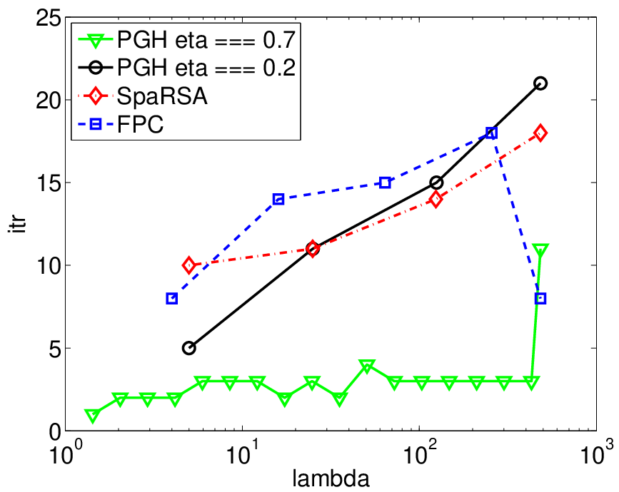
As mentioned in the introduction, similar approximate homotopy/continuation methods have been studied for the -LS problem. Here we compare the PGH method with two most relevant ones: sparse reconstruction by separable approximation (SpaRSA) [WNF09], and fixed point continuation (FPC) [HYZ08]. In particular, the same proximal gradient method (5) is used in each iteration of both SpaRSA and FPC. Their continuation strategies are both based on reducing by a constant factor at each stage.
SpaRSA uses Barzilai-Borwein (spectral) method for choosing at each step. More specifically, at each iteration the parameter is initialized as
then it is increased by a constant factor until an acceptance criterion is satisfied. When both and are sparse, say for some integer , then the above satisfies
According to Section 2.3, such a line search method is able to exploit the restricted strong convexity, similar as the PGH method. However, the line-search acceptance criterion of SpaRSA is different from PGH, and they also have different stopping criteria for each homotopy stage. Global geometric convergence of either SpaRSA or FPC has not been established.
In our numerical experiments, we used the monotone version of SpaRSA with continuation, which we call SpaRSA-MC. For FPC, we used a more recent implementation by the authors of [HYZ08] that also employs Barzilai-Borwein line search, which is called FPC-BB. In fact FPC-BB solves the equivalent problem
where . Moreover, it further scales the matrix so that the maximum singular value is at most . In Figures 4 and 5, the results of FPC-BB are plotted after we reversed the scalings in order to compare with other methods. Default options were used in both methods. SpaRSA-MC reduces the value of roughly with an factor , and FPC-BB has an equivalent factor . For meaningful comparison, we also present the results for PGH with , in addition to its default value . The same relative precision was used in both cases for PGH.
Figure 4 shows the numerical results of different algorithms on the same random instance studied in Figure 1. They demonstrate similar numerical properties, and SpaRSA-MC is especially similar to PGH with . The numbers of iterations at each continuation stage depend on the specific stopping criteria used in different algorithms. In Figure 4, the small number of iterations in the final stage of FPC-BB is a result of the relatively loose precision specified in its default options, which is also reflected in Figure 4. According to Figure 3, the aggressive decreasing factors used in SpaRSA and FPC can lead to less sparse iterates along the solution path, thus relatively slower convergence at the intermediate stages. But their overall iteration counts are comparable to PGH with .

We also conducted experiments with random problem instances where the vector is not sufficiently sparse. Figure 5 shows the objective gap of different methods when solving a random problem instance generated similarly as the one studied in Figure 1. The only difference is that here the vector has nonzero elements. In this case, all methods demonstrate sub-linear convergence. SpaRSA-M is the monotone version of SpaRSA without continuation. FPC-BB terminated prematurely because its default accuracy for its stopping criterion is too low. FPC-BB-HA is the result after we set a much higher accuracy in calling the FPC-BB method. It looks that the same higher accuracy is used in all the homotopy stages, so the number of inner iterations increased for each stage. We see that the algorithms with homotopy continuation still perform better than their single-stage counterparts, but the improvements are less impressive. Instead, the accelerated gradient methods ADG and ADGH outperform other methods by a big margin.
5.2 Basis pursuit


Finally we present an experiment of solving the basis pursuit (BP) problem (8) using PGH, and compare it with FPC and SpaRSA. In this experiment, the matrix is a partial FFT matrix. More specifically, we choose rows at random from the FFT matrix with . The vector has nonzero entries at only randomly chosen coordinates, and they were generated independently from the normal distribution with zero mean and unit variance. Then we set in the BP problem (i.e., this is the noise-free case with ).
In this case, since is a matrix with complex numbers, we need to replace all the real transpose in the algorithms with Hermitian transpose, and replace the soft-thresholding operator in (7) with
where denotes the modulus of the complex number [WNF09].
The solution to the BP problem (8) can be obtained by letting in the -LS problem (1). In order to use the PGH method, we set . The same parameter was also used in calling SpaRSA-MC and FPC-BB. Figure 6 shows the numerical results. Again we observe remarkable resemblance between these methods in Figure 6. However, in Figure 6, we see the recovery error of SpaRSA-MC stayed at the level while its objective function in Figure 6 converged to zero faster than other methods. The reason is that SpaRSA has a fixed accuracy requirement for all continuation stages except for the last one. As shown in Figure 6, when becomes very small, this constant accuracy is always reached within one iteration, and such a low accuracy is too loose for the algorithm to track the homotopy path closely. Therefore, even though the objective function converges to zero quickly, the recovery error stayed large. This is also confirmed through the denser continuation stages in the second half of SpaRSA-MC, as shown in Figure 6. To see this, we note that the adaptive continuation used in SpaRSA is
If is an accurate solution for the stage , then we have and thus with as the default value. When this is not the case, then can be notably larger than , and thus the regularization parameter reduces at a much slower pace. Similar as PGH, FPC-BB sets the accuracy for each continuation stage to be proportional to the regularization parameter, but for a different stopping criterion. With our choice of stopping criterion, , the number of inner iterations for each continuation stage stayed roughly constant along the homotopy path.
This example also demonstrates the advantage of PGH and other approximate homotopy continuation methods over the exact homotopy path-following methods [OPT00a, OPT00b, EHJT04]. Figure 6 shows that high-precision recovery can be obtained by PGH in less than iterations (which corresponds to roughly matrix-vector multiplications). This is much more efficient than using the exact homotopy path-following methods, which need to track at least breakpoints. In addition, their computational cost at each break point is much higher than a matrix-vector multiplication.
6 Conclusion and discussions
This paper studied a proximal-gradient homotopy method for solving the -regularized least squares problems, focusing on its important application in sparse recovery. For such applications, the objective function is not strongly convex; hence the standard single-stage proximal gradient methods can only obtain relatively slow convergence rate. However, we have shown that under suitable conditions for sparse recovery, all iterates of the proximal-gradient homotopy method along the solution path are sparse. With this extra sparsity structure, the objective function becomes effectively strongly convex along the solution path, and thus a geometric rate of convergence can be achieved using the homotopy approach. Our theoretical analysis are supported by several numerical experiments.
We commented in the numerical experiments that accelerated gradient methods cannot automatically exploit restricted strong convexity. As discussed in [Nes04, Section 2.2] and [Nes07], they need to explicitly use the strong convexity parameter, or a non-trivial lower bound of it, to obtain geometric convergence. In order to exploit restricted strong convexity in the -LS problem with , accelerated gradient methods need an extra facility to come up with an explicit estimate of the restricted convexity parameter on the fly. Nesterov gave some suggestions along this direction in [Nes07], and strategies such as periodic restart have been studied recently [GLW09, BCG11]. However, an in-depth investigation on this matter is beyond the scope of this paper.
References
- [ANW11] A. Agarwal, S. N. Negahban, and M. J. Wainwright. Fast global convergence of gradient methods for high-dimensional statistical recovery. Technical Report arXiv:1104.4824v1, arXiv, 2011.
- [BBC11] S. R. Becker, J. Bobin, and E. J. Candès. NESTA: A fast and accurate first-order method for sparse recovery. SIAM Journal on Imaging Sciences, 4(1):1–39, 2011.
- [BCG11] S. R. Becker, E. J. Candès, and M. C. Grant. Templates for convex cone problems with applications to sparse signal recovery. Mathematical Programming Computation, 3(3):165–218, 2011.
- [BDE09] A. M. Bruckstein, D. L. Donoho, and M. Elad. From sparse solutions of systems of equations to sparse modeling of signals and images. SIAM Review, 51(1):34–81, 2009.
- [BDF07] J. M. Bioucas-Dias and M. A. T. Figueiredo. A new TwIST: Two-step iterative shrinking/thresholding algorithms for image restoration. IEEE Transactions on Image Processing, 16(12):2992–3004, 2007.
- [BRT09] P. Bickel, Y. Ritov, and A. Tsybakov. Simultaneous analysis of Lasso and Dantzig selector. Annals of Statistics, 37:1705–1732, 2009.
- [BT09] A. Beck and M. Teboulle. A fast iterative shrinkage-threshold algorithm for linear inverse problems. SIAM Journal on Imaging Sciences, 2(1):183–202, 2009.
- [CDS98] S. S. Chen, D. L. Donoho, and M. A. Saunders. Atomic decomposition by basis pursuit. SIAM Journal on Scientific Computing, 20(1):33–61, 1998.
- [CRT06] E. J. Candès, J. Romberg, and T. Tao. Robust uncertainty principles: Exact signal reconstruction from highly incomplete frequency information. IEEE Transactions on Information Theory, 52(2):489–509, February 2006.
- [CT05] E. J. Candès and T. Tao. Decoding by linear programming. IEEE Transactions on Information Theory, 51(12):4203–4215, December 2005.
- [CT06] E. J. Candès and T. Tao. Near-optimal signal recovery from random projections: universal encoding strategies? IEEE Transactions on Information Theory, 52(12):5406–5425, December 2006.
- [CT07] E. J. Candes and T. Tao. The dantzig selector: statistical estimation when is much larger than (with discussion). Annals of Statistics, 35:2313–2404, 2007.
- [CW05] P. Combettes and V. Wajs. Signal recovery by proximal forward-backward splitting. SIAM Journal on Multiscale Modeling and Simulation, 4(4):1168–1200, 2005.
- [DDM04] I. Daubechies, M. Defriese, and C. De Mol. An iterative thresholding algorithm for linear inverse problems with a sparsity constraint. Communications on Pure and Applied Mathematics, 57(11):1413–1457, 2004.
- [DET06] D. L. Donoho, M. Elad, and V. Temlyakov. Stable recovery of sparse overcomplete representations in the presence of noise. IEEE Transactions on Information Theory, 52(1):6–18, January 2006.
- [DMA97] G. Davis, S. Mallat, and M. Avellaneda. Adaptive greedy approximations. Journal of Constructive Approximation, 13(1):57–98, 1997.
- [Don06] D. L. Donoho. Compressed sensing. IEEE Transactions on Information Theory, 52(4):1289–1306, April 2006.
- [DT08] D. L. Donoho and Y. Tsaig. Fast solution of -norm minimization problems when the solution may be sparse. IEEE Transactions on Information Theory, 54(11):4789–4812, November 2008.
- [EHJT04] B. Efron, T. Hastie, I. Johnstone, and R. Tibshirani. Least angle regression (with discussion). Annals of Statistics, 32:407–499, 2004.
- [GLW09] M. Gu, L.-H. Lim, and C. J. Wu. ParNes: A rapidly convergent algorithm for accurate recovery of sparse and approximately sparse signals. Preprint. arXiv:0911.0492, 2009.
- [HYZ08] E. T. Hale, W. Yin, and Y. Zhang. Fixed-point continuation for -minimization: Methodology and convergence. SIAM Journal on Optimization, 19(3):1107–1130, 2008.
- [KKL+07] S.-J. Kim, K. Koh, M. Lustig, S. Boyd, and D. Gorinevsky. An interior-point method for large-scale -regularized least squares. IEEE Journal on Selected Topics in Signal Processing, 1(4):606–617, December 2007.
- [Kol09] V. Koltchinskii. The dantzig selector and sparsity oracle inequalities. Bernoulli, 15:799–828, 2009.
- [LT92] Z.-Q. Luo and P. Tseng. On the linear convergence of descent methods for convex essentially smooth minimization. SIAM Journal on Control and Optimization, 30(2):408–425, 1992.
- [MB06] N. Meinshausen and P. Bühlmann. High dimensional graphs and variable selection with the lasso. Annals of Statistics, 34:1436–1462, 2006.
- [Nes83] Yu. Nesterov. A method for solving a convex programming problem with convergence rate . Soviet Mathematics - Doklady, 27(2):372–376, 1983.
- [Nes96] Yu. Nesterov. Long-step strategies in interior-point primal-dual methods. Mathematical Programming, 76:47–94, 1996.
- [Nes04] Yu. Nesterov. Introductory Lectures on Convex Optimization: A Basic Course. Kluwer, Boston, 2004.
- [Nes05] Yu. Nesterov. Smooth minimization of nonsmooth functions. Mathematical Programming, 103(1):127–152, 2005.
- [Nes07] Yu. Nesterov. Gradient methods for minimizing composite objective function. CORE discussion paper 2007/76, Center for Operations Research and Econometrics, Catholic University of Louvain, Belgium, September 2007.
- [NT09] D. Needell and J. A. Tropp. CoSaMP: Iterative signal recovery from incomplete and inaccurate samples. Applied and Computational Harmonic Analysis, 26(3):301–321, 2009.
- [OPT00a] M. Osborne, B. Presnell, and B. Turlach. A new approach to variable selection in least squares problems. IMA Journal of Numerical Analysis, 20:389–404, 2000.
- [OPT00b] M. Osborne, B. Presnell, and B. Turlach. On the lasso and its dual. Journal of Computational and Graphical Statistics, 9(2):319–337, 2000.
- [Roc70] R. T. Rockafellar. Convex Analysis. Princeton University Press, 1970.
- [Tib96] R. Tibshirani. Regression shrinkage and selection via the lasso. Journal of the Royal Statistical Society: Series B (Statistical Methodology), 58:267–288, 1996.
- [Tro04] J. A. Tropp. Greedy is good: Algorithmic results for sparse approximation. IEEE Transactions on Information Theory, 50(10):2231–2242, 2004.
- [Tro06] J. A. Tropp. Just relax: convex programming methods for identifying sparse signals in noise. IEEE Transactions on Information Theory, 52:1030–1051, 2006.
- [Tse08] P. Tseng. On accelerated proximal gradient methods for convex-concave optimization. Manuscript submitted to SIAM Journal on Optimization, 2008.
- [TVW05] B. A. Turlach, W. N. Venables, and S. J. Wright. Simultaneous variable selection. Technometrics, 47:349–363, 2005.
- [TW10] J. A. Tropp and S. J. Wright. Computational methods for sparse solution of linear inverse problems. Proceedings of the IEEE, 98(6):948–958, 2010.
- [vdBF08] E. van den Berg and M. P. Friedlander. Probing the Pareto frontier for basis pursuit solutions. SIAM Journal on Scientific Computing, 31(2):980–912, 2008.
- [vdGB09] S. van de Geer and P. Bühlmann. On the conditions used to prove oracle results for the lasso. Electronic Journal of Statistics, 3:1360–1392, 2009.
- [Wai09] M. J. Wainwright. Sharp thresholds for noisy and high–dimensional recovery of sparsity using –constrained quadratic programming (lasso). IEEE Transactions on Information Theory, 55:2183–2202, 2009.
- [WNF09] S. J. Wright, R. D. Nowad, and M. A. T. Figueiredo. Sparse reconstruction by separable approximation. IEEE Transactions on Signal Processing, 57(7):2479–2493, July 2009.
- [WYGZ10] Z. Wen, W. Yin, D. Goldfarb, and Y. Zhang. A fast algorithm for sparse reconstruction based on shrinkage, subspace optimization and continuation. SIAM Journal on Scientific Computing, 32(4):1832–1857, 2010.
- [YOGD08] W. Yin, S. Osher, D. Goldfarb, and J. Darbon. Bregman iterative algorithms for -minimization with applications to compressed sensing. SIAM Journal on Imaging Science, 1(1):143–168, 2008.
- [ZH08] C.-H. Zhang and J. Huang. The sparsity and bias of the lasso selection in high–dimensional linear regression. Annals of Statistics, 36:1567–1594, 2008.
- [Zha09] T. Zhang. Some sharp performance bounds for least squares regression with regularization. Annals of Statistics, 37:2109–2144, 2009.
- [ZY06] P. Zhao and B. Yu. On model selection consistency of lasso. Journal of Machine Learning Research, 7:2541–2567, 2006.