Can a Lamb Reach a Haven Before Being Eaten by Diffusing Lions?
Abstract
We study the survival of a single diffusing lamb on the positive half line in the presence of diffusing lions that all start at the same position to the right of the lamb and a haven at . If the lamb reaches this haven before meeting any lion, the lamb survives. We investigate the survival probability of the lamb, , as a function of and the respective initial positions of the lamb and the lions, and . We determine analytically for the special cases of and . For large but finite , we determine the unusual asymptotic form whose leading behavior is , with . Simulations of the capture process very slowly converge to this asymptotic prediction as reaches .
pacs
02.50.Cw, 05.40.-a, 05.50.+q1 Introduction
We investigate the one-dimensional diffusive capture process in which a marked particle — a “lamb” — diffuses on the positive half line in the presence of independently diffusing predators — “lions” — that are all initially at . If the lamb meets any lion, the lamb is killed. Additionally, the origin is a haven for the lamb. If the lamb reaches the haven before meeting any of the lions, then the lamb survives. We are interested in the survival probability of the lamb as a function of the starting positions of the two species, as well as on the number of lions.
This model is a natural counterpoint to the well-studied capture process of a single diffusing lamb in the presence of independent, diffusing lions on the infinite line [1, 2, 3, 4, 5]. In the most interesting situation where the lions are all on one side of the lamb, the survival probability of the lamb asymptotically decays as a power-law in time, , with the exponent exhibiting a non-trivial dependence on the number of lions and also on the diffusivities of each animal. For simplicity, the case where the diffusivities of all animals are the same (and set to one) is normally considered. The initial positions of the lamb and the lions are irrelevant in this asymptotic behavior.
For this diffusive capture on the infinite line, the exponent is known exactly only for and : and [1, 2, 3, 4, 5, 6, 7]. The latter result shows that even though the two lions are independent, their effect on the capture process is not, since . For the case , a mapping to an equivalent electrostatic problem leads to the accurate estimate [8]. For , the value of has been estimated with moderate accuracy only for a few values of [1]; however, it is known that for , so that the average lifetime of the lamb is finite [9]. Because grows more slowly than linearly with , each additional lion has a progressively weaker influence on the capture process. As , both asymptotic and rigorous arguments give [2, 3, 4]. Parenthetically, the capture process with lions sited on both sides of the lamb is much more efficient than in the one-sided system. For lions with approximately equal numbers of them on either side of the lamb, the lamb survival probability asymptotically decays as , with growing linearly with for large .

In this work, we incorporate the new feature of a haven at and ask whether the lamb can reach the haven before meeting any of the lions. If the haven is reached, we say that the lamb survives (Fig. 1). Our goal is to determine how the ultimate survival probability depends on the initial positions of the lamb and all the lions, and , respectively, as well as on the number of lions. As we shall see, the survival probability depends on rather than on and separately and thus we write the ultimate survival probability as . Our main result is that has an unusual form whose leading behavior is , but this behavior does not become apparent until becomes of the order of .
We begin by solving the simplest and exactly-soluble case of one lion in Sect. 2. We also outline the formal solution to the problem for any number of lions. In Sect. 3 we treat the extreme case where the number of lions is infinite, so that the lion that is closest to the lamb moves ballistically. We then investigate arbitrary in Sect. 4. When is large, we can replace the lions by a single “closest lion” that moves deterministically. We develop approximation schemes to estimate in this large- limit. We also present numerical results for the survival probability in Sect. 5. A straightforward simulation of the random-walk motion of the particles is prohibitively slow when is large, and we present two alternative approaches that are considerably more efficient and allow us to probe the survival probability in the regime where is extremely large — of the order of . Finally, in Sect. 6, we summarize and also discuss some natural and intriguing extensions of the model.
2 Exact Analysis
2.1 One Lion
As a preliminary, we can readily solve the case of one lamb at and one lion at for the general situation where the diffusivities of the two species are distinct — for the lamb and for the lion. We compute the survival probability that the lamb reaches the haven at before being eaten by the lion, , by mapping the coordinates of the lamb and the lion on the line to diffusion in a two-dimensional wedge, from which the survival probability follows easily.
It is convenient to transform from the coordinates to and . In the - plane, the motions of the lamb and lion on the half line can be viewed as the isotropic diffusion of a fictitious composite particle with unit diffusivity [7, 10]. If reaches zero while the condition is always satisfied, the lamb survives (Fig. 2). Conversely, if at some time (corresponding to ) while always remains positive, then the lamb has been eaten by the lion before the haven is reached.

In the - plane, the initial position of the composite particle is
corresponding to the polar angle
| (1) |
The allowed region for the composite particle is a wedge of opening angle
| (2) |
We want the probability that the composite particle first hits the line (corresponding to the lamb reaching the haven) without hitting the line . This probability satisfies the Laplace equation [10]
for , with boundary conditions and . Clearly the solution is a function that linearly interpolates between 0 and 1 in the angular direction, so that the ultimate survival probability is [10, 11]
| (3) |

As is obvious from Fig. 3, the closer that the lamb starts to the haven the more likely it is to survive. Moreover, as can be inferred from Fig. 2, the best strategy for the lamb to survive for a given initial condition is to diffuse quickly. As the diffusivity of the lamb increases, the wedge angle in Fig. 2 approaches while the starting position of the fictitious particle in the plane moves close to the axis, i.e., closer to the haven. Finally notice that in the limit (stationary lion), the survival probability decays linearly with .
As a byproduct of the wedge mapping, we can immediately determine the probability that the lamb is still diffusing — that is, the lamb has not yet reached the haven and has not yet been eaten by the lion. This situation corresponds to the fictitious particle having not yet reached either of the sides of an infinite wedge defined by and . In the isotropic - coordinates, this wedge has opening angle (Fig. 2), and the survival probability asymptotically decays as . In particular, when , then (see Eq. (2)), and the survival probability asymptotically decays as .
2.2 Formal Solution for General
The reasoning given above can be readily generalized to map the problem of a diffusing lamb in the presence of diffusing lions to a single diffusing fictitious particle in dimensions, with boundary conditions that reflect the lamb reaching the haven or being eaten by a lion. For simplicity, we set the diffusivities of the lamb and the lions to one. We first discuss the case of two lions; the generalization to any number of lions is immediate.
Suppose that the lamb is initially at and that the two lions are initially at . The lamb survives if it reaches without meeting either of the lions on the way to . We now map the diffusion of the three interacting particles on the positive half line to the isotropic diffusion of a composite particle at in three dimensions, with constraints that correspond to the interactions in the lamb-lion system. By this mapping, the allowed region for the composite particle is defined by , corresponding to the lamb not yet reaching the refuge, as well as by and , corresponding to the lamb not yet eaten by either of the lions. This defines a wedge-shaped region that are delineated by three planar sides that is known as a Weyl chamber [12].
The survival of the lamb corresponds to the composite particle first hitting the plane of the Weyl chamber without hitting either of the planes and . By the equivalence between first-passage and electrostatics [10], this survival probability of the lamb coincides with the electrostatic potential at the initial point of the composite particle, with the boundary conditions on the plane , and on the planes and . This same mapping works for any number of lions and constitutes the formal solution. Unfortunately, the analytical solution to this potential problem does not seem tractable for more than one lion (i.e., three or more particles), although some extreme value electrostatic properties have recently been exactly solved for the three-particle problem [14].
3 Infinite Number of Lions
When the number of lions is infinite, the lion closest to the haven — the closest lion — would reach the haven at an infinitesimal time. However, it is instructive to consider the related problem in which each lion undergoes a nearest-neighbor random walk. In this case, the position of the last lion inexorably moves one lattice spacing to the left in each time step. For this system, we determine the ultimate survival probability by writing the backward Kolmogorov equation [10] for and then applying scaling to solve this equation. The result should correspond to that obtained for diffusing lions in the limit of very large .
To write the backward equation, we consider the evolution of the system over a small time interval during which the lamb moves to and the boundary moves to , where is the boundary velocity. That is, the position of the lamb evolves by the Langevin equation , where is Gaussian white noise with zero mean, , and correlation . We now view the new positions of the lamb and the boundary after the time interval as the initial conditions for the subsequent evolution. Thus , where the average is over the initial noise . Expanding the right-hand side of this recursion to lowest non-vanishing order in each variable and using the properties of delta-correlated noise, we obtain the backward equation
| (4) |
for , with the boundary conditions and . To solve this equation we make the scaling ansatz (with ) to give the ordinary differential equation for :
| (5) |
subject to the boundary conditions and ; here the prime denotes differentiation with respect to .
Integrating and applying the boundary conditions gives
| (6) |
In the limit , this expression reduces to
| (7) |
with . The primary feature of this result is that the lamb survival probability is non-zero only within a thin boundary layer where the starting position satisfies . Outside this layer the lamb is almost surely eaten by one of the lions.
4 Asymptotics for Large
The capture process also simplifies when the number of lions is finite but large, because the position of the closest lion becomes progressively more deterministic as increases, even though each individual lion undergoes independent Brownian motion. Thus we only need to consider the ultimate survival of the lamb in the presence of a single effective predator [13] — the closest lion — that moves systematically towards the lamb (Fig. 4). We now exploit this physical picture to give a heuristic argument for the ultimate survival probability of the lamb.

When all the lions start at , the average number of lions at is
We estimate the location of the closest lion, , by demanding that . This criterion gives [4]
| (8) |
where
| (9) |
and . Thus to lowest order, . At a critical time the closest lion has reached the haven at and the capture process is necessarily finished — either the lamb has been killed or it has reached the haven. Notice that although must be large for the closest lion to move deterministically, cannot be too large. As discussed in the previous section, if each lion undergoes a nearest-neighbor random walk, the closest lion moves deterministically to the left with speed when is sufficiently large. For Eq. (8) to be valid, we therefore require (to lowest order) that , or . Using and for a nearest-neighbor random walk, the last lion moves deterministically as only when . For , the last lion moves with constant unit speed toward the lamb.
We now crudely estimate the ultimate survival probability of the lamb as the total probability flux that reaches up to time in the semi-infinite system without any additional constraints. This integrated flux represents an upper bound for the survival probability for large because this estimate includes lamb trajectories that could intersect the trajectory of the last lion and then reach the haven. For a diffusing particle that starts at , the flux to an absorbing boundary at the origin at time is: [10]
Consequently, the probability for the lamb to get trapped at the origin up to time (corresponding to the lamb reaching the haven and surviving) satisfies the bound
| (10) |
Here we have used the substitution to transform to a Gaussian integral, as well as the lowest-order approximation and .
From the asymptotic form , we thus obtain an upper bound for the ultimate survival probability that has the unusual functional form
| (11) |
Consistent with basic intuition, is a decreasing function of and also decreases as with fixed. It should be emphasized that Eq. (11) applies in the limit of , which is extremely hard to achieve by direct simulation. For example, if the lamb starts halfway between the haven and the lions (), then for , the argument of the complementary error function is ; for , . Conversely to reach requires . Notice also that Eq. (10) matches the survival probability given by Eq. (7) for a ballistically-moving boundary when reaches a critical value for which the completion time also equals .
More rigorously, we should also incorporate the absorbing boundary condition at , corresponding to the lamb getting eaten by the closest lion. This problem of a fixed absorbing boundary at and a moving absorbing boundary at does not seem readily soluble, however. Instead, we investigate a related model in which the boundary motion mimics that of the closest lion, but is engineered to be soluble. As we shall show, the ultimate survival probability for this alternative problem has a qualitatively similar dependence on system parameters as Eq. (11). Consider the toy model in which the closest lion coordinate is (compared to , with , for diffusing lions). These two boundaries satisfy the inequality and both reach the origin at the same time when . Thus the toy model remains an upper bound for the true survival probability.
It is again convenient to treat the evolution of the system in the two-dimensional space . Let be the probability that the lamb successfully reaches the haven, where and denote the initial positions of the lamb and the boundary respectively. Following the same approach as in Sec. 3, we write the backward equation for . In a small time interval the lamb moves to , where is Gaussian white noise with zero mean, and the boundary moves to , where is the boundary speed. The survival probability now satisfies , and expanding the right-hand side to lowest order gives the backward equation
| (12) |
for , with the boundary conditions and . To solve (12) we make the scaling ansatz , with , where and , and find that the scaling function satisfies
| (13) |
for , with the boundary conditions and ; here the prime denotes differentiation with respect to . Integrating once gives , and integrating again gives
| (14) |
where the constants are determined by the boundary conditions. Substituting in and gives the asymptotic behavior
| (15) |
This upper bound has the same asymptotic behavior as (11) and suggests that the heuristic approach should be quite accurate.
5 Simulations
We now present simulation results for the lamb-lion-haven system. While a direct simulation is simple to code, it becomes prohibitively slow when is large. We have therefore developed two complimentary approaches to determine the survival probability in the large- limit.
5.1 Probability Propagation
Probability propagation is well-suited for probing the case of , where we replace the position of the closest lion by a deterministic absorbing boundary, , that moves according to Eq. (8). Here, the constant can be chosen as the mean or most probable position of the closest lion or any other reasonable positional metric. We choose to set , which is the leading behavior in Eq. (8). The omission of higher-order corrections, which slightly decrease , lead to a more slowly-moving boundary and a correspondingly slightly larger survival probability. Thus probability propagation should provide a lower bound to the true survival probability.
Let be the probability that the lamb is at at time . At each time step, the probability in the interior region propagates according to ; here is the largest integer less than . At the edge sites and . Probability elements that reach either or do not propagate further and remain in place. Probability propagation continues until reaches . The total probability at at this termination time gives the survival probability of the lamb.
We used probability propagation to obtain for up to . We used quadruple precision variables to ensure accuracy of the probability values throughout the propagation. The initial value of was chosen to be the smallest such that finite-size effects were imperceptible — this ranged from for small to for the largest values.
5.2 Event-Driven Simulation
A naive simulation is simply to move every lion and the lamb by at each time step, an approach which is prohibitively slow for large . However, there is no need to simulate every single random-walk step, particularly if the lamb is far from both the haven and nearest lion. This motivates using an event-driven simulation, in which we propagate all particles over a time that corresponds to a finite fraction of the time needed for a reaction to actually occur — either the lamb reaching the haven or getting eaten by the closest lion.
Let be the minimum of the distances between the lamb and the nearest lion, and between the lamb and the haven. We could move every particle according to a binomial distribution of steps because there is no possibility that the lamb meets any of the lions or reaches the haven during this update. However, this approach is unnecessarily stringent because each particle moves a typical distance that is only of the order of . Thus we increment the number of steps by , where
| (16) |
and move every particle according to a binomial distribution of steps. Note that these update rules match at the crossover separation . After each such update, we check if the lamb has reached or crossed over the position of the haven or that of any lion, in which case the simulation is finished.
For , and the lamb cannot reach either the haven or any lion during the update; this part of the simulation is exact. For , there is a non-zero probability that the lamb trajectory could cross the haven or a lion trajectory and then cross back during the update. However, by choosing appropriately, the probability of error due to such crossing trajectories can be made vanishingly small. We found that gave an excellent compromise between accuracy and efficiency. We also checked that simulations results with the update rule (16) are essentially identical with exact results that arise by choosing in the update rule (16).
5.3 Results
In Fig. 5(a) we show the dependence of the ultimate survival probability versus scaled initial position for up to , with realizations for each data point, from event-driven simulations. For , these survival probabilities gradually converge, as increases, to a limiting curve that corresponds to the system where the last lion moves ballistically. The lions are all initially at and we verified that the survival probability depends only on the ratio , without any explicit finite- dependence. This independence on emerges when and thus we focus on the smallest system () where finite-size effects are negligible.


We also examined the dependence of on for fixed to test the asymptotic power-law behavior of Eq. (11). Our analytical prediction matches the simulation quite well for (Fig. 5)(b). However, a small but slowly growing discrepancy arises as is increased beyond 0.5. The source of this discrepancy is that the heuristic derivation of Sec. 4 ignores the existence the absorbing boundary caused by the last lion. When approaches 1, the lamb starts sufficiently close to the last lion that the assumption of ignoring the boundary caused by the last lion is no longer valid.
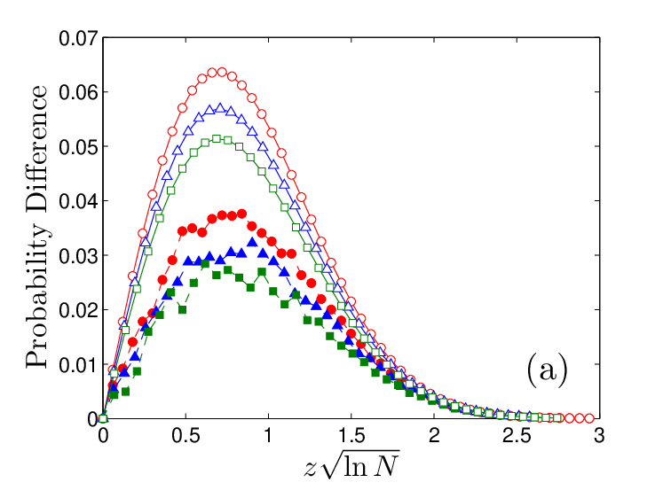
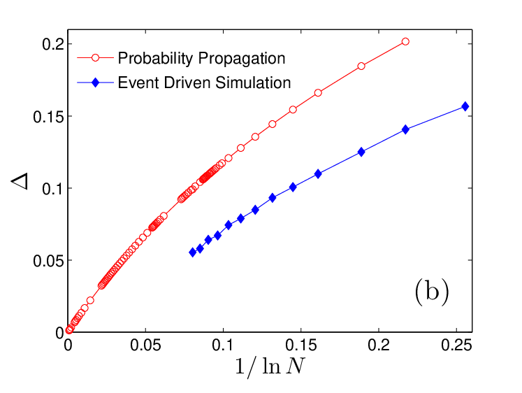
Finally, we compare our two simulation approaches with each other and with our our heuristic prediction from Eq. (10). By construction, the event-driven simulation is more accurate because it explicitly follows the stochastic motion of the lamb and the lions. Our heuristic prediction (10) provides an upper bound for large , but this regime is not feasible to simulate with the event-driven algorithm. Conversely, the probability propagation simulation can be implemented for arbitrarily large but suffers from systematic error because it assumes the closest lion position to be deterministic.
Figure 6(a) illustrates the convergence of the simulation results to Eq. (10) where the difference between the simulated value of and is plotted as a function of for representative values. We quantify this difference by , where , with , is the area beneath the analytic survival curve and similarly for the area beneath the simulated curve. Figure 6(b) shows that as for the probability propagation algorithm. A similar, but not identical convergences arises in the event-driven simulation, but the method cannot reach the large- regime. These results provide strong evidence that the survival probability is indeed given by as .
6 Outlook
The presence of a haven adds an intriguing element to the classic capture process of a single lamb in the presence of diffusing lions. Now the basic question is whether the lamb can reach safety at the haven before it is eaten by one of the lions. We investigated the dependence of the ultimate survival probability of the lamb, , on the number of lions and also on the initial positions of the lamb () and the lions (all at , for simplicity). By a rough heuristic argument, we found that has the asymptotic behavior , and this function has the unusual leading behavior , where . It is remarkable that a simplistic approach gives such an unusual and rich result. However, the approach to this asymptotic regime is extremely slow and it is necessary to simulate a system that corresponds to of the order of lions before the asymptotic behavior becomes apparent.
It is natural to ask about the properties of the ultimate survival probability in higher dimensions. For diffusive capture in an unbounded system, the case of one dimension is the most interesting. However, the presence of a haven now makes the higher-dimensional problem nontrivial. For example, in two dimensions, a natural setting would be a diffusing prey, diffusing predators, and a circular haven of radius centered at the origin. Because of the recurrence of diffusion in two dimensions, the prey will eventually reach the haven if there are no predators, but the mean time to reach the haven is infinite. What happens when predators exist? How does the survival probability depend on the number of predators and on the initial positions of the prey and predators? How long does it take for the capture process to end? Another interesting two-dimensional geometry is a semi-infinite planar haven. Finally, in three dimensions, the transience of diffusion could lead to very different properties for the survival probability than in two dimensions.
We thank Paul Krapivsky for helpful discussions and advice. AG, NKP, and SR thank NSF grant DMR-0906504 for partial financial support of this research. S.N.M. acknowledges partial support by ANR grant 2011-BS04-013-01 WALKMAT and by the Indo-French Centre for the Promotion of Advanced Research under Project 4604-3.
References
References
- [1] M. Bramson and D. Griffeath, “Capture problems for coupled random walks,” in Random Walks, Brownian Motion, and Interacting Particle Systems: A Festschrift in Honor of Frank Spitzer, R. Durrett and H. Kesten, eds., pp. 153–188 (Birkhäuser, Boston, 1991).
- [2] H. Kesten, “An absorption problem for several Brownian motions”, in Seminar on Stochastic Processes, 1991, E. Çinlar, K. L. Chung, and M. J. Sharpe, eds. (Birkhäuser, Boston, 1992).
- [3] P. L. Krapivsky and S. Redner, “Kinetics of a diffusive capture process: Lamb besieged by a pride of lions”, J. Phys. A 29, 5347–5357 (1996).
- [4] S. Redner and P. L. Krapivsky, “Capture of the lamb: Diffusing predators seeking a diffusing prey”, Am. J. Phys. 67, 1277–1283 (1999).
- [5] P. L. Krapivsky, S. N. Majumdar, A. Rosso, “Maximum of N Independent Brownian Walkers till the First Exit From the Half Space”, J. Phys. A: Math. Theor. 43, 315001 (2010).
- [6] M. E. Fisher, “Walks, walls, wetting, and melting”, J. Stat. Phys. 34, 667–729 (1984).
- [7] M. E. Fisher and M. P. Gelfand, “The reunions of three dissimilar vicious walkers”, J. Stat. Phys. 53, 175 (1988).
- [8] D. ben-Avraham, B. M. Johnson, C. A. Monaco, P. L. Krapivsky, and S. Redner, “Ordering of Random Walks: The Leader and the Laggard” J. Phys. A 36, 1789–1799 (2003).
- [9] W. V. Li and Q.-M. Shao, “Capture time of Brownian pursuits”, Probab. Theor. Relat. Fields 122, 494-508 (2002).
- [10] S. Redner, “A Guide to First-Passage Processes” (Cambridge University Press, Cambridge, 2001).
- [11] H. S. Carslaw and J. C. Jaeger, Conduction of Heat in Solids (Clarendon Press, Oxford, U.K., 1959).
- [12] D. J. Grabiner, “Brownian motion in a Weyl chamber, non-colliding particles, and random matrices”, Ann. Inst. H. Poincaré (B) Prob. Stat. 35, 177–204 (1999).
- [13] L. Breiman, “First exit time from the square root boundary,” Proc. Fifth Berkeley Symp. Math. Statist. and Probab. 2, 9–16 (1966); H. E. Daniels, “The minimum of a stationary Markov superimposed on a U-shape trend,” J. Appl. Prob. 6, 399–408 (1969); K. Uchiyama, “Brownian first exit from sojourn over one sided moving boundary and application,” Z. Wahrsch. verw. Gebiete 54, 75–116 (1980); P. Salminen, “On the hitting time and the exit time for a Brownian motion to/from a moving boundary,” Adv. Appl. Prob. 20, 411–426 (1988).
- [14] S. N. Majumdar and A. J. Bray, “Maximum distance between the leader and the laggard for three Brownian walkers”, J. Stat. Mech. P08023 (2010).