跳到论文正文
W Papers独立论文阅读器 arXiv:1203.2912 论文正文 计算阅读时间 · 0%
引用这篇论文根据当前论文元数据生成,正式投稿前建议核对。


License: arXiv.org perpetual non-exclusive license
arXiv:1203.2912v1 [math.NA] 13 Mar 2012

Radial basis functions for the solution of hypersingular operators on open surfacesThanks: Supported by FONDECYT-Chile under grant number 1110324 and UNSW FRG Grant number PS24436.

Norbert Heuer ††thanks: Facultad de Matemáticas, Pontificia Universidad Católica de Chile, Avenida Vicuña Mackenna 4860, Santiago, Chile. email: nheuer@mat.puc.cl.    Thanh Tran ††thanks: School of Mathematics and Statistics, The University of New South Wales, Sydney 2052, Australia. email: thanh.tran@unsw.edu.au.
Abstract

We analyze the approximation by radial basis functions of a hypersingular integral equation on an open surface. In order to accommodate the homogeneous essential boundary condition along the surface boundary, scaled radial basis functions on an extended surface and Lagrangian multipliers on the extension are used. We prove that our method converges quasi-optimally. Approximation results for scaled radial basis functions indicate that, for highly regular radial basis functions, the achieved convergence rates are close to the one of low-order conforming boundary element schemes. Numerical experiments confirm our conclusions.

Key words: boundary element method, radial basis functions, non-conforming method, Lagrangian multiplier

AMS Subject Classification: 65N55, 65N38

1 Introduction

This paper is about the approximation by radial basis functions of functions in Sobolev spaces subject to a Dirichlet boundary condition. To the best of our knowledge this is the first time that such functions are used and analyzed for problems with essential boundary condition. There arise several difficulties when imposing or analyzing trace conditions for spaces of radial basis functions (RBF):

  • (i)

    Radial basis functions are selected by their center points on the domain of interest. Their supports are generally large and overlap with those of several other RBF. Considering boundary traces of RBF close to the boundary, their shapes and supports on the boundary vary continuously with the position of the center on the domain. Therefore, the structure and basis functions of trace spaces is not fixed, neither is there a fixed intrinsic basis on the boundary.

  • (ii)

    Analysis of stability and approximation properties of RBF and related operators is based on Fourier analysis in the so-called native space. Depending on the choice of RBF, this native space is a Sobolev space of high regularity. Considering domains with, e.g., Lipschitz boundary there is no obvious way to employ arguments from native spaces to traces.

  • (iii)

    Traditional arguments from finite element analysis (like locality and equivalence of norms in finite dimensional spaces) are difficult to apply to RBF for their very nature. That is why the native space is of central importance. In trace spaces of RBF, however, such arguments (locality, equivalence of norms) are even harder to come by due to the varying structure of functions, cf. (i).

In this paper we propose a mixed method employing RBF and finite elements (as Lagrangian multipliers) to deal with essential boundary conditions. We analyze non-conforming approximations with scaled radial basis functions in a fractional order Sobolev space with homogeneous essential boundary condition. The underlying model problem is the hypersingular integral equation on an open surface for the solution of the Laplacian in the exterior domain (with Neumann boundary condition). The energy space of this problem is a Sobolev space of order 1/21/2 on the surface with the condition that functions can be extended by 00.

The analysis comprises two principal problems. One is the approximation theory for radial basis functions in fractional order Sobolev spaces with essential boundary condition; the other is the necessity of a non-conforming approach in a fractional order Sobolev space.

Radial basis functions are well studied, mainly for the interpolation of scattered data but also for the approximation of partial differential equations. For some overviews see, e.g., [7, 21, 22, 30]. In particular, Wendland studies the approximation for second order equations with Neumann boundary condition [29], and multiresolution properties of scaled radial basis functions [31]. Neumann boundary conditions allow for extending the approximation analysis to the full space where standard arguments apply (using the native space of the radial basis functions). To the best of our knowledge there exists no analysis for boundary value problems with essential boundary condition. In this paper we tackle this problem for a Sobolev space of order 1/21/2. Let us note that spherical radial basis functions (on the closed sphere) in this space are well analyzed, see [20, 19, 25, 26]. In this paper we consider the case of a general open smooth surface with the particular problem of incorporating an essential boundary condition.

This boundary condition appears in a natural way when dealing with boundary integral equations on open surfaces. In the case of a Neumann problem the unknown of the integral equation is the jump across the surface of the solution to the exterior problem [24]. Since the jump of this solution vanishes at the boundary of the surface the underlying energy space has to incorporate this condition. However, there is no well-defined trace operator in the corresponding Sobolev space H1/2H^{1/2} so that this condition appears as part of the norm; the corresponding space is denoted by H~1/2\tilde{H}^{1/2}, sometimes also referred to as H001/2H^{1/2}_{00}. Conforming approximations require that approximating functions vanish at the boundary of the surface. This causes no difficulty when using piecewise polynomials; the corresponding method is called the boundary element method (BEM). When using radial basis functions, however, a conforming and converging method is difficult to construct since conformity requires that the centers of the functions stay away from the boundary. This requirement is unrealistic because in practice centers can stay close to or even on the boundary. We thus propose a non-conforming approach where the essential boundary condition is implemented by a Lagrangian multiplier. For the BEM such procedures have been studied, with resulting almost quasi-optimal convergence, see [10, 12, 14]. Here we use a different approach where the surface is extended to a larger surface so that supports of radial basis functions remain inside the extended surface. We then use a Lagrangian multiplier on the extended part of the surface to make the approximating functions vanish there. This idea is similar to a penalty or fictitious domain method.

An overview of the rest of the paper is as follows. In the next section we recall Sobolev spaces, present our model problem and give an equivalent mixed formulation which will be used for the discretization with radial basis functions. In Section 3 we introduce scaled radial basis functions and the discrete scheme, and we list our theoretical results which are proved in subsequent sections. In Section 4 we prove the quasi-optimal convergence of our scheme, and in Section 5 we present an approximation theory for scaled radial basis functions. In Section 6 we resume our theoretical results and conclude that the resulting convergence order tends to the one of a standard BEM when the regularity of the radial basis functions grows. This conclusion is based on numerical evidence of boundedness of an additional stability term that arises in our analysis. Finally, in Section 7 we report on some numerical results that underline the convergence properties of our method.

Throughout the paper, the symbol ≲\lesssim will be used in the usual sense. In short, a⁡(h,k,r)≲b⁡(h,k,r)a(h,k,r)\lesssim b(h,k,r) when there exists a constant C>0C>0 independent of discretization or scaling parameters hh, kk, rr (except otherwise noted) such that a⁡(h,k,r)≤C​b​(h,k,r)a(h,k,r)\leq Cb(h,k,r). The double inequality a≲b≲aa\lesssim b\lesssim a is simplified to a≃ba\simeq b.

2 Model problem and mixed formulation

In order to introduce our model problem and its mixed formulation we need to recall the definition of some Sobolev spaces.

We consider standard Sobolev spaces of integer order and define fractional order spaces by interpolation, using the real K-method, see [2]. For a Lipschitz domain Ω\Omega and 0<s<10<s<1 we use the spaces

Hs​(Ω):=[L2​(Ω),H1​(Ω)]s,H~s​(Ω):=[L2​(Ω),H01​(Ω)]sH^{s}(\Omega):=[L_{2}(\Omega),H^{1}(\Omega)]_{s},\qquad\tilde{H}^{s}(\Omega):=[L_{2}(\Omega),H_{0}^{1}(\Omega)]_{s}

where the norm in H01​(Ω)H_{0}^{1}(\Omega) is the H1​(Ω)H^{1}(\Omega)-semi-norm. For orders s>1s>1, the spaces are defined by interpolation between L2​(Ω)L_{2}(\Omega) and a correspondingly higher integer order Sobolev space. For s∈(0,1/2)s\in(0,1/2), ∥⋅∥H~s​(Ω)\|\cdot\|_{\tilde{H}^{s}(\Omega)} and ∥⋅∥Hs​(Ω)\|\cdot\|_{H^{s}(\Omega)} are equivalent norms whereas for s∈(1/2,1)s\in(1/2,1) there holds H~s​(Ω)=H0s​(Ω)\tilde{H}^{s}(\Omega)=H_{0}^{s}(\Omega), the latter space consisting of functions whose traces on ∂Ω\partial\Omega vanish. Generally, H~s​(Ω)\tilde{H}^{s}(\Omega) consists of functions which are continuously extendable by zero onto a larger domain. For s>0s>0 the spaces H−s​(Ω)H^{-s}(\Omega) and H~−s​(Ω)\tilde{H}^{-s}(\Omega) are the dual spaces of H~s​(Ω)\tilde{H}^{s}(\Omega) and Hs​(Ω)H^{s}(\Omega), respectively. Similarly we define Sobolev spaces on surfaces.

In the analysis we need some more norms. In the literature different definitions of Sobolev norms are being used and we have to be careful to check their equivalence when combining different results. Apart from interpolation norms, on a domain Σ⊂IR2\Sigma\subset\mbox{\rm I\kern-1.79993ptR}^{2} (Σ=IR2\Sigma=\mbox{\rm I\kern-1.79993ptR}^{2} is allowed), we also need the Sobolev-Slobodeckij norm. For s=m+σs=m+\sigma with integer m≥0m\geq 0 and σ∈(0,1)\sigma\in(0,1) we define

‖v‖s,Σ:=(‖v‖m,Σ2+|v|s,Σ2)1/2\|v\|_{s,\Sigma}:=\Bigl(\|v\|_{m,\Sigma}^{2}+|v|_{s,\Sigma}^{2}\Bigr)^{1/2}

with semi-norm

|v|s,Σ=(∑|α|=m∫Σ∫Σ|Dα​v​(x)−Dα​v​(y)|2|x−y|2+2​σ​𝑑x​𝑑y)1/2|v|_{s,\Sigma}=\Bigl(\sum_{|\alpha|=m}\int_{\Sigma}\int_{\Sigma}\frac{|D^{\alpha}v(x)-D^{\alpha}v(y)|^{2}}{|x-y|^{2+2\sigma}}\,dx\,dy\Bigr)^{1/2}

and multi-index α=(α1,α2)\alpha=(\alpha_{1},\alpha_{2}). Here, ∥⋅∥m,Σ\|\cdot\|_{m,\Sigma} is the standard Sobolev norm, as before,

‖v‖m,Σ2=∑|α|≤m‖Dα​v‖L2​(Σ)2.\|v\|_{m,\Sigma}^{2}=\sum_{|\alpha|\leq m}\|D^{\alpha}v\|_{L_{2}(\Sigma)}^{2}.

Our model problem is as follows. For given f∈H−1/2(Γ)f\in H^{-1/2}(\Gamma) find ϕ∈H~1/2​(Γ)\phi\in\tilde{H}^{1/2}(\Gamma) such that

Wϕ(x):=−14​π∂∂𝐧x∫Γϕ(y)∂∂𝐧y1|x−y|dSy=f(x),x∈Γ.W\phi(x):=-\frac{1}{4\pi}\frac{\partial}{\partial{\bf n}_{x}}\int_{\Gamma}\phi(y)\frac{\partial}{\partial{\bf n}_{y}}\frac{1}{|x-y|}\,dS_{y}=f(x),\quad x\in\Gamma. (2.1)

Here, Γ\Gamma is a smooth open surface with piecewise smooth Lipschitz boundary and 𝐧{\bf n} is a normal unit vector on Γ\Gamma. We refer to [24] for the setting of this model problem and the error analysis of its conforming approximation by boundary elements.

Later we will extend Γ\Gamma to a larger surface and use the notation WW for the hypersingular operator on the extended surface as well.

For ease of presentation we restrict ourselves to the case of a flat surface and assume that Γ\Gamma is a polygonal Lipschitz domain in IR2\mbox{\rm I\kern-1.79993ptR}^{2}. Then, in particular, Γ\Gamma satisfies an interior cone condition.

We intend to approximate the solution ϕ\phi to (2.1) by radial basis functions. The conformity condition that approximation spaces be subspaces of H~1/2​(Γ)\tilde{H}^{1/2}(\Gamma) requires that discrete functions vanish at the boundary γ\gamma of Γ\Gamma. This means that points for the definition of radial basis functions could not be freely selected since one wants to take radial basis functions of uniform radius which cannot be too small, as is well known. In order to be able to freely choose center points we extend the domain Γ\Gamma to a larger domain Γ~{\tilde{\Gamma}} so that, for a given parameter r>0r>0 there holds dist(γ,γ~)>r\mathop{\rm dist}\nolimits(\gamma,{\tilde{\gamma}})>r. Here, γ~{\tilde{\gamma}} denotes the boundary of Γ~{\tilde{\Gamma}} and we assume that Γ~{\tilde{\Gamma}} is at least Lipschitz. Later, the parameter rr will be the scaling parameter for the radial basis functions. Scaling the basis functions appropriately, we will be able to select center points anywhere on Γ¯\bar{\Gamma} and the discrete spaces of radial basis functions will be subspaces of H~1/2​(Γ~)\tilde{H}^{1/2}({\tilde{\Gamma}}).

A standard variational formulation of (2.1) is: find ϕ∈H~1/2​(Γ)\phi\in\tilde{H}^{1/2}(\Gamma) such that

⟨W​ϕ,ψ⟩Γ=⟨f,ψ⟩Γ∀ψ∈H~1/2​(Γ).\langle W\phi,\psi\rangle_{\Gamma}=\langle f,\psi\rangle_{\Gamma}\qquad\forall\psi\in\tilde{H}^{1/2}(\Gamma). (2.2)

However, to give the setting for the discrete method we consider a non-standard formulation on the extended domain Γ~{\tilde{\Gamma}}: find (ϕ~,λ)∈H~1/2(Γ~)×H~γ−1/2(Γc)(\tilde{\phi},\lambda)\in\tilde{H}^{1/2}({\tilde{\Gamma}})\times\tilde{H}^{-1/2}_{\gamma}({\Gamma^{c}}) such that

⟨W​ϕ~,ψ⟩Γ~−⟨λ,ψ⟩Γc=⟨f0,ψ⟩Γ~∀ψ∈H~1/2​(Γ~),⟨μ,ϕ~⟩Γc=0∀μ∈H~−1/2γ(Γc).\begin{array}[]{llll}\langle W\tilde{\phi},\psi\rangle_{\tilde{\Gamma}}-\langle\lambda,\psi\rangle_{\Gamma^{c}}&=&\langle f^{0},\psi\rangle_{\tilde{\Gamma}}&\quad\forall\psi\in\tilde{H}^{1/2}({\tilde{\Gamma}}),\\ \langle\mu,\tilde{\phi}\rangle_{\Gamma^{c}}&=&0&\quad\forall\mu\in\tilde{H}^{-1/2}_{\gamma}({\Gamma^{c}}).\end{array} (2.3)

Here, Γc:=Γ~∖Γ¯{\Gamma^{c}}:={\tilde{\Gamma}}\setminus\bar{\Gamma} with boundary γ∪γ~\gamma\cup{\tilde{\gamma}} consisting of two connected components (Γc{\Gamma^{c}} is an annular domain). Also, we use the following notation for the dual space:

H~γ−1/2(Γc):=(H~∂Γc∖γ1/2(Γc))′=(H~γ~1/2(Γc))′\tilde{H}^{-1/2}_{\gamma}({\Gamma^{c}}):=\left(\tilde{H}^{1/2}_{\partial{\Gamma^{c}}\setminus\gamma}({\Gamma^{c}})\right)^{\prime}=\left(\tilde{H}^{1/2}_{\tilde{\gamma}}({\Gamma^{c}})\right)^{\prime}

where

H~γ~1/2​(Γc):=[L2​(Γc),H0,γ~1​(Γc)]1/2\tilde{H}^{1/2}_{\tilde{\gamma}}({\Gamma^{c}}):=[L_{2}({\Gamma^{c}}),H_{0,{\tilde{\gamma}}}^{1}({\Gamma^{c}})]_{1/2}

with H0,γ~1​(Γc)H_{0,{\tilde{\gamma}}}^{1}({\Gamma^{c}}) being the space of H1​(Γc)H^{1}({\Gamma^{c}})-functions whose traces on γ~{\tilde{\gamma}} vanish. In particular, any ψ∈H~γ~1/2​(Γc)\psi\in\tilde{H}^{1/2}_{\tilde{\gamma}}({\Gamma^{c}}) is extendable by zero to a function ψ0∈H1/2​(IR2∖Γ¯)\psi^{0}\in H^{1/2}(\mbox{\rm I\kern-1.79993ptR}^{2}\setminus\bar{\Gamma}). Below, we will use this notation, instead of Γc{\Gamma^{c}}, also on extended domains Γkc{\Gamma^{c}_{k}} depending on a mesh parameter kk.

Note that H~1/2​(Γ)=H~γ1/2​(Γ)\tilde{H}^{1/2}(\Gamma)=\tilde{H}^{1/2}_{\gamma}(\Gamma) and

H~γ−1/2(Γ)=(H~∅1/2(Γ))′=(H1/2(Γ))′=H~−1/2(Γ).\tilde{H}^{-1/2}_{\gamma}(\Gamma)=(\tilde{H}^{1/2}_{\emptyset}(\Gamma))^{\prime}=(H^{1/2}(\Gamma))^{\prime}=\tilde{H}^{-1/2}(\Gamma).

Also, for ff defined on Γ\Gamma, f0f^{0} denotes the extension of ff by 00 onto Γ~{\tilde{\Gamma}} (we will use this generic notation throughout for the extension to any domain which will be clear from the particular situation).

There obviously holds the following result.

Proposition 2.1

Let f∈H−1/2(Γ)f\in H^{-1/2}(\Gamma) so that f0∈H−1/2(Γ~)f^{0}\in H^{-1/2}({\tilde{\Gamma}}). Then the formulations (2.2) and (2.3) are equivalent and have unique solutions. There holds ϕ~|Γ=ϕ\tilde{\phi}|_{\Gamma}=\phi and ϕ~|Γ~∖Γ¯=0\tilde{\phi}|_{{\tilde{\Gamma}}\setminus\bar{\Gamma}}=0, i.e. ϕ~=ϕ0\tilde{\phi}=\phi^{0}, and λ=W​ϕ0\lambda=W\phi^{0} on Γ~∖Γ¯{\tilde{\Gamma}}\setminus\bar{\Gamma}.

3 Discrete method and theoretical results

We solve (2.3) by approximating ϕ~\tilde{\phi} by radial basis functions and λ\lambda by piecewise constant functions. To this end let Φ\Phi denote a non-negative radial basis function centered around x=0x=0 with compact support B¯​(0,1)\bar{B}(0,1) (B⁡(y,s)B(y,s) is the disc {x∈IR2;|x−y|<s}\{x\in\mbox{\rm I\kern-1.79993ptR}^{2};\;|x-y|<s\}) and Fourier transform

ℱ⁡(Φ)​(ξ)=Φ^​(ξ)≃(1+|ξ|2)−τ,ξ∈IR2{\cal F}(\Phi)(\xi)=\hat{\Phi}(\xi)\simeq(1+|\xi|^{2})^{-\tau},\quad\xi\in\mbox{\rm I\kern-1.79993ptR}^{2} (3.1)

for τ>1\tau>1. The parameter τ\tau is fixed throughout. We consider scaled radial basis functions

Φr​(x):=r−2​Φ​(x/r),r>0,x∈IR2,\Phi_{r}(x):=r^{-2}\Phi(x/r),\quad r>0,\quad x\in\mbox{\rm I\kern-1.79993ptR}^{2},

so that

Φ^r​(ξ)≃(1+r2​|ξ|2)−τ.\hat{\Phi}_{r}(\xi)\simeq(1+r^{2}|\xi|^{2})^{-\tau}. (3.2)

Selecting a finite set of nodes X:={x1,…,xN}⊂Γ¯X:=\{x_{1},\ldots,x_{N}\}\subset\bar{\Gamma} we define the discrete space

HX,r:=span{ϕ1,…,ϕN}whereϕi​(x):=Φr​(x−xi),i=1,…,N.H_{X,r}:=\mathop{\rm span}\nolimits\{\phi_{1},\ldots,\phi_{N}\}\quad\mbox{where}\quad\phi_{i}(x):=\Phi_{r}(x-x_{i}),\ i=1,\ldots,N.

Since the nodes can be near to or even on the boundary of Γ\Gamma, the supports of the scaled radial basis functions are not necessarily subsets of Γ\Gamma. We extend Γ\Gamma to a fixed larger domain Γ~{\tilde{\Gamma}} satisfying supp(ϕi)⊂Γ~\mathop{\rm supp}\nolimits(\phi_{i})\subset{\tilde{\Gamma}} for any ϕi∈HX,r\phi_{i}\in H_{X,r}, any chosen set XX and any r∈(0,r0]r\in(0,r_{0}] where r0>0r_{0}>0 is fixed.

We also need the mesh norm hX,Σh_{X,\Sigma} (for Σ⊂IR2\Sigma\subset\mbox{\rm I\kern-1.79993ptR}^{2}) defined by

hX,Σ:=supx∈Σdist(x,X).h_{X,\Sigma}:=\sup_{x\in\Sigma}\mathop{\rm dist}\nolimits(x,X).

We extend Γ\Gamma by a strip of shape-regular, quasi-uniform quadrilateral elements TT of diameter proportional to kk as indicated in Figure 3.1. We require that the minimum diameter and length of the smallest edge on γ\gamma are not smaller than kk. With shape-regularity we refer to elements whose minimum (respectively, maximum) interior angles are bounded from below (respectively, from above) by a positive constant less than π\pi. We denote this mesh by 𝒯k{\cal T}_{k} and require that

𝒯k{\cal T}_{k} is geometrically conforming with γ\gamma: each element T∈𝒯kT\in{\cal T}_{k} has either one or more entire edges in common with γ\gamma, or T¯∩γ\bar{T}\cap\gamma is a vertex of Γ\Gamma and of TT. The latter case happens at most once for each vertex of Γ\Gamma.

The extended domain is denoted by Γ~k{\tilde{\Gamma}_{k}}:

Γ~k=interior⁡(Γ¯∪{T¯;T∈𝒯k}).{\tilde{\Gamma}_{k}}={\rm interior}(\bar{\Gamma}\cup\{\bar{T};\;T\in{\cal T}_{k}\}).

In the following, we choose the mesh size kk accordingly to the scaling parameter rr: k>rk>r and kk is small enough so that Γ~k⊂Γ~{\tilde{\Gamma}_{k}}\subset{\tilde{\Gamma}} and no element touches two vertices of Γ\Gamma. The assumption k>rk>r guarantees that the supports of the scaled radial basis functions are within Γ~k{\tilde{\Gamma}_{k}}.

We introduce the notation Γkc{\Gamma^{c}_{k}} for the strip Γ~k∖Γ¯{\tilde{\Gamma}_{k}}\setminus\bar{\Gamma} and γ~k:=∂Γ~k{\tilde{\gamma}_{k}}:=\partial{\tilde{\Gamma}_{k}} for the boundary of Γ~k{\tilde{\Gamma}_{k}}.

Let us collect the assumptions we have made:

  • (A1)

    The scaling parameter rr and mesh parameter kk are bounded, r∈(0,r0]r\in(0,r_{0}], r<k<k0r<k<k_{0}. 𝒯k{\cal T}_{k} is a quasi-uniform mesh of shape-regular quadrilaterals of diameter proportional to kk with minimum diameter not less than kk and with edges on γ\gamma of length not less than kk. Moreover, 𝒯k{\cal T}_{k} is geometrically conforming with γ\gamma and no element touches two vertices of Γ\Gamma.

Refer to caption
Figure 3.1: Domain Γ\Gamma extended by strip Γkc{\Gamma^{c}_{k}} with mesh 𝒯k{\cal T}_{k}.

Now, for the approximation of the Lagrangian multiplier λ\lambda we take piecewise constant functions,

Mk:={μ∈L2(Γkc);μ|T=const∀T∈𝒯k}.M_{k}:=\{\mu\in L_{2}({\Gamma^{c}_{k}});\;\mu|_{T}=const\ \forall T\in{\cal T}_{k}\}.

Using these discrete spaces, the boundary element scheme with radial basis functions and Lagrangian multiplier for the approximate solution of (2.3) is: find (ϕN,λk)∈HX,r×Mk(\phi_{N},\lambda_{k})\in H_{X,r}\times M_{k} such that

⟨W​ϕN,ψ⟩Γ~k−⟨λk,ψ⟩Γkc=⟨f0,ψ⟩Γ~k∀ψ∈HX,r,⟨μ,ϕN⟩Γkc=0∀μ∈Mk.\begin{array}[]{llll}\langle W\phi_{N},\psi\rangle_{\tilde{\Gamma}_{k}}-\langle\lambda_{k},\psi\rangle_{\Gamma^{c}_{k}}&=&\langle f^{0},\psi\rangle_{\tilde{\Gamma}_{k}}&\quad\forall\psi\in H_{X,r},\\ \langle\mu,\phi_{N}\rangle_{\Gamma^{c}_{k}}&=&0&\quad\forall\mu\in M_{k}.\end{array} (3.3)

Defining the subspace

VX,r:={ψ∈HX,r;⟨μ,ψ⟩Γkc=0∀μ∈Mk},V_{X,r}:=\{\psi\in H_{X,r};\;\langle\mu,\psi\rangle_{\Gamma^{c}_{k}}=0\quad\forall\mu\in M_{k}\},

and assuming an inf-sup condition for the bilinear form ⟨⋅,⋅⟩Γkc\langle\cdot,\cdot\rangle_{\Gamma^{c}_{k}} on Mk×HX,rM_{k}\times H_{X,r}, (3.3) is equivalent to: find ϕN∈VX,r\phi_{N}\in V_{X,r} such that

⟨W​ϕN,ψ⟩Γ~k=⟨f0,ψ⟩Γ~k∀ψ∈VX,r.\langle W\phi_{N},\psi\rangle_{\tilde{\Gamma}_{k}}=\langle f^{0},\psi\rangle_{\tilde{\Gamma}_{k}}\quad\forall\psi\in V_{X,r}.

Apart from assumption (A1) we will need some more properties of XX for our analysis. We must be able to fix a constant function on any given element by testing with a radial basis function.

To make this precise, let 𝒞⊂𝒯k{\cal C}\subset{\cal T}_{k} denote the set of elements TT such that the closure T¯\overline{T} intersects γ\gamma only at a vertex of Γ\Gamma. For instance, in the example of Figure 3.1 there are five such elements, at five of the six convex vertices. Further we denote ℰ:=𝒯k∖𝒞{\cal E}:={\cal T}_{k}\setminus{\cal C}. Then we assume:

  • (A2)

    ∀T∈ℰ∃xi∈X:supp(ϕi)∩Γkc⊂T\displaystyle\forall T\in{\cal E}\quad\exists x_{i}\in X:\quad\mathop{\rm supp}\nolimits(\phi_{i})\cap{\Gamma^{c}_{k}}\subset T

  • (A3)

    ∀T∈𝒞:T has exactly two neighborsT1,T2∈ℰ,\displaystyle\forall T\in{\cal C}:\quad T\mbox{ has exactly two neighbors}\ T_{1},T_{2}\in{\cal E},
        ∃xi∈X:supp(ϕi)∩T≠∅,supp(ϕi)∩T~=∅​∀T~∈𝒯k∖{T,T1,T2}\displaystyle\qquad\quad\exists x_{i}\in X:\quad\mathop{\rm supp}\nolimits(\phi_{i})\cap T\not=\emptyset,\quad\mathop{\rm supp}\nolimits(\phi_{i})\cap\tilde{T}=\emptyset\ \forall\tilde{T}\in{\cal T}_{k}\setminus\{T,T_{1},T_{2}\}

For any T∈𝒯kT\in{\cal T}_{k} there may be more than one xi∈Xx_{i}\in X satisfying either (A2) or (A3). We will denote one of these points xix_{i} by xi⁡(T)x_{i(T)}.

Moreover, we assume that there is substantial overlap between HX,rH_{X,r} and MkM_{k}:

  • (A4)

    ∃κ>0:meas(supp(ϕi⁡(T))∩T)≥κ​meas(supp(ϕi⁡(T)))=κ​π​r2∀T∈𝒯k\displaystyle\exists\kappa>0:\quad\mathop{\rm meas}\nolimits(\mathop{\rm supp}\nolimits(\phi_{i(T)})\cap T)\geq\kappa\,\mathop{\rm meas}\nolimits(\mathop{\rm supp}\nolimits(\phi_{i(T)}))=\kappa\,\pi r^{2}\quad\forall T\in{\cal T}_{k}

Remark 3.1

Note that the discrete scheme is defined on the domain Γ~k{\tilde{\Gamma}_{k}} which depends on kk. But this causes no difficulty since, under the assumptions made, all the domains Γ~k{\tilde{\Gamma}_{k}} can be extended to the fixed domain Γ~{\tilde{\Gamma}} and the spaces involved allow for extension by zero of their elements to Γ~{\tilde{\Gamma}}. More precisely, there holds

HX,r⊂H~1/2(Γ~k)⊂H~1/2(Γ~),Mk⊂H~γ−1/2(Γkc)⊂H~γ−1/2(Γc)H_{X,r}\subset\tilde{H}^{1/2}({\tilde{\Gamma}_{k}})\subset\tilde{H}^{1/2}({\tilde{\Gamma}}),\quad M_{k}\subset\tilde{H}^{-1/2}_{\gamma}({\Gamma^{c}_{k}})\subset\tilde{H}^{-1/2}_{\gamma}({\Gamma^{c}})

where the latter inclusions are to be understood as the uniformly continuous injections of the respective extension by zero.

Theoretical results.

Based on assumptions (A1)–(A4) we prove the following results.

  • •

    The discrete scheme (3.3) converges quasi-optimally; see Theorem 4.1.

  • •

    The error of the best approximation by radial basis functions in the constrained space VX,rV_{X,r} (mean value zero on elements of the extension) can be bounded by the error of the best approximation in the unconstrained space HX,rH_{X,r} on Γ\Gamma plus a stability term; see Theorem 4.3.

  • •

    We prove an error estimate for the best approximation by scaled radial basis functions (Theorem 5.4) which appears to be sharp according to our numerical results in Section 7.

We are unable to show an appropriate bound for the stability term |ψ|Ht​(Γkc)|\psi|_{H^{t}({\Gamma^{c}_{k}})} in Theorem 4.3. Based on our numerical tests, however, we conjecture that this term is appropriately bounded so that we conclude for the choice k≃r≃hX,Γ1−t/τk\simeq r\simeq h_{X,\Gamma}^{1-t/\tau} the overall error estimate

‖ϕ−ϕN‖H1/2​(Γ)≤C​hX,Γ(t−1/2−ϵ)​(1−t/τ)ϵ>0,t∈(1/2,1].\|\phi-\phi_{N}\|_{H^{1/2}(\Gamma)}\leq C\,h_{X,\Gamma}^{(t-1/2-\epsilon)(1-t/\tau)}\quad\epsilon>0,t\in(1/2,1]. (3.4)

The constant CC would depend on tt, ϵ\epsilon and τ\tau but not on XX and hX,Γh_{X,\Gamma} under the assumptions made. We refer to Section 6, in particular (6.6), for more details.

Remark 3.2

In our case of an open surface Γ\Gamma, the solution ϕ\phi of (2.1) has strong singularities along γ\gamma. This limits the convergence order of approximation schemes. Measuring regularity in standard Sobolev spaces, the hh-version of the standard boundary element method with quasi-uniform meshes (and mesh size hh) converges like

‖ϕ−ϕh‖H~1/2​(Γ)≲ht−1/2​‖ϕ‖Ht​(Γ),\|\phi-\phi_{h}\|_{\tilde{H}^{1/2}(\Gamma)}\lesssim h^{t-1/2}\|\phi\|_{H^{t}(\Gamma)}, (3.5)

cf. [27]. Since ϕ∈Ht​(Γ)\phi\in H^{t}(\Gamma) for any t<1t<1 but ϕ∉H1​(Γ)\phi\not\in H^{1}(\Gamma) in general there is an upper limit 1/21/2 for the convergence order in hh. An optimal error estimate making use of the type of appearing singularities is

‖ϕ−ϕh‖H~1/2​(Γ)≲h1/2,\|\phi-\phi_{h}\|_{\tilde{H}^{1/2}(\Gamma)}\lesssim h^{1/2},

again for quasi-uniform meshes, see [4]. In our case of radial basis functions the mesh size hh corresponds to the mesh norm hX,Γh_{X,\Gamma} and for quasi-uniform distribution of nodes this parameter is equivalent to hh for quasi-uniform meshes. The estimate (3.4) exactly reflects the error estimate (3.5) for large τ\tau. Selecting sufficiently smooth radial basis functions, which corresponds to large τ\tau, one gets as close as wanted to the convergence order 1/21/2. The use of lower regularity of radial basis functions results in a lower convergence order. Our numerical experiments reported below confirm the predicted influence of τ\tau.

4 Quasi-optimal convergence

We prove the quasi-optimal convergence of (3.3) for the approximation of ϕ\phi. Later, in Section 5 we study the approximation problems for ϕ\phi and λ\lambda to derive convergence orders. We do not bound the Galerkin error for the Lagrangian multiplier λ\lambda since, on the one hand, proving a discrete inf-sup condition for the bilinear forms ⟨⋅,⋅⟩Γkc\langle\cdot,\cdot\rangle_{\Gamma^{c}_{k}} is an open problem and, on the other hand, the function λ\lambda is of no physical interest. We will therefore analyze (3.3) without using a discrete inf-sup condition.

Theorem 4.1

Let the assumptions (A1)–(A3) be satisfied. Then there exists a unique solution to (3.3) and there holds the quasi-optimal error estimate

∥ϕ0−ϕN∥H~1/2​(Γ~k)≲infψ∈VX,r∥ϕ0−ψ∥H~1/2​(Γ~k)+infμ∈Mk∥λ−μ∥H~−1/2γ(Γck).\|\phi^{0}-\phi_{N}\|_{\tilde{H}^{1/2}({\tilde{\Gamma}_{k}})}\lesssim\inf_{\psi\in V_{X,r}}\|\phi^{0}-\psi\|_{\tilde{H}^{1/2}({\tilde{\Gamma}_{k}})}+\inf_{\mu\in M_{k}}\|\lambda-\mu\|_{\tilde{H}^{-1/2}_{\gamma}({\Gamma^{c}_{k}})}.

Proof. The existence and uniqueness of (ϕN,λk)∈HX,r×Mk(\phi_{N},\lambda_{k})\in H_{X,r}\times M_{k} follows from the Babuška-Brezzi theory. Specifically, uniformly in kk,

  • (i)

    ⟨W⋅,⋅⟩Γ~k\langle W\cdot,\cdot\rangle_{\tilde{\Gamma}_{k}} is bounded:

    ⟨W​v,ψ⟩Γ~k=⟨W​v0,ψ0⟩Γ~≲‖v0‖H~1/2​(Γ~)​‖ψ0‖H~1/2​(Γ~)≃‖v‖H~1/2​(Γ~k)​‖ψ‖H~1/2​(Γ~k)\langle Wv,\psi\rangle_{\tilde{\Gamma}_{k}}=\langle Wv^{0},\psi^{0}\rangle_{\tilde{\Gamma}}\lesssim\|v^{0}\|_{\tilde{H}^{1/2}({\tilde{\Gamma}})}\|\psi^{0}\|_{\tilde{H}^{1/2}({\tilde{\Gamma}})}\simeq\|v\|_{\tilde{H}^{1/2}({\tilde{\Gamma}_{k}})}\|\psi\|_{\tilde{H}^{1/2}({\tilde{\Gamma}_{k}})} (4.1)

    for any v,ψ∈H~1/2​(Γ~k)v,\psi\in\tilde{H}^{1/2}({\tilde{\Gamma}_{k}})

  • (ii)

    ⟨W⋅,⋅⟩Γ~k\langle W\cdot,\cdot\rangle_{\tilde{\Gamma}_{k}} is elliptic:

    ⟨W​ψ,ψ⟩Γ~k=⟨W​ψ0,ψ0⟩Γ~≳‖ψ0‖H~1/2​(Γ~)2≃‖ψ‖H~1/2​(Γ~k)2∀ψ∈H~1/2​(Γ~k)\langle W\psi,\psi\rangle_{\tilde{\Gamma}_{k}}=\langle W\psi^{0},\psi^{0}\rangle_{\tilde{\Gamma}}\gtrsim\|\psi^{0}\|_{\tilde{H}^{1/2}({\tilde{\Gamma}})}^{2}\simeq\|\psi\|_{\tilde{H}^{1/2}({\tilde{\Gamma}_{k}})}^{2}\quad\forall\psi\in\tilde{H}^{1/2}({\tilde{\Gamma}_{k}}) (4.2)
  • (iii)

    ⟨⋅,⋅⟩Γkc\langle\cdot,\cdot\rangle_{\Gamma^{c}_{k}} is bounded:

    ⟨μ,ψ⟩Γkc≤∥μ∥H~−1/2γ(Γck)∥ψ∥H~γ~k1/2​(Γkc)≤∥μ∥H~−1/2γ(Γck)∥ψ∥H~1/2​(Γ~k)\langle\mu,\psi\rangle_{\Gamma^{c}_{k}}\leq\|\mu\|_{\tilde{H}^{-1/2}_{\gamma}({\Gamma^{c}_{k}})}\|\psi\|_{\tilde{H}^{1/2}_{\tilde{\gamma}_{k}}({\Gamma^{c}_{k}})}\leq\|\mu\|_{\tilde{H}^{-1/2}_{\gamma}({\Gamma^{c}_{k}})}\|\psi\|_{\tilde{H}^{1/2}({\tilde{\Gamma}_{k}})} (4.3)

    for any μ∈H~γ−1/2(Γkc)\mu\in\tilde{H}^{-1/2}_{\gamma}({\Gamma^{c}_{k}}) and ψ∈H~1/2​(Γ~k)\psi\in\tilde{H}^{1/2}({\tilde{\Gamma}_{k}})

  • (iv)

    The linear form defined by f0f^{0} is bounded, i.e.

    ⟨f0,ψ⟩Γ~k≤∥f0∥H−1/2(Γ~k)∥ψ∥H~1/2​(Γ~k)≲∥f0∥H−1/2(Γ~)∥ψ∥H~1/2​(Γ~k)∀ψ∈H~1/2(Γ~k).\langle f^{0},\psi\rangle_{\tilde{\Gamma}_{k}}\leq\|f^{0}\|_{H^{-1/2}({\tilde{\Gamma}_{k}})}\|\psi\|_{\tilde{H}^{1/2}({\tilde{\Gamma}_{k}})}\lesssim\|f^{0}\|_{H^{-1/2}({\tilde{\Gamma}})}\|\psi\|_{\tilde{H}^{1/2}({\tilde{\Gamma}_{k}})}\quad\forall\psi\in\tilde{H}^{1/2}({\tilde{\Gamma}_{k}}).

Here, we used several uniform norm-equivalences, e.g. ‖v‖H~1/2​(Γ~k)≃‖v0‖H~1/2​(Γ~)\|v\|_{\tilde{H}^{1/2}({\tilde{\Gamma}_{k}})}\simeq\|v^{0}\|_{\tilde{H}^{1/2}({\tilde{\Gamma}})} since H~1/2​(Γ~k)\tilde{H}^{1/2}({\tilde{\Gamma}_{k}}) (resp., H~1/2​(Γ~)\tilde{H}^{1/2}({\tilde{\Gamma}})) is defined by interpolation between L2​(Γ~k)L_{2}({\tilde{\Gamma}_{k}}) and H01​(Γ~k)H_{0}^{1}({\tilde{\Gamma}_{k}}) (resp, between L2​(Γ~)L_{2}({\tilde{\Gamma}}) and H01​(Γ~)H_{0}^{1}({\tilde{\Gamma}})), and

‖v‖H01​(Γ~k)=|v|H1​(Γ~k)=|v0|H1​(Γ~)=‖v0‖H01​(Γ~)∀v∈H01​(Γ~k).\|v\|_{H_{0}^{1}({\tilde{\Gamma}_{k}})}=|v|_{H^{1}({\tilde{\Gamma}_{k}})}=|v^{0}|_{H^{1}({\tilde{\Gamma}})}=\|v^{0}\|_{H_{0}^{1}({\tilde{\Gamma}})}\qquad\forall v\in H_{0}^{1}({\tilde{\Gamma}_{k}}).

Rather than proving a discrete inf-sup condition for the bilinear form ⟨⋅,⋅⟩Γkc\langle\cdot,\cdot\rangle_{\Gamma^{c}_{k}} we only show injectivity. More precisely,

  • (v)

    ⟨⋅,⋅⟩Γkc\langle\cdot,\cdot\rangle_{\Gamma^{c}_{k}} is discrete injective:

    (μ∈Mk:⟨μ,ψ⟩Γkc=0∀ψ∈HX,r)⇒μ=0\Bigl(\mu\in M_{k}:\quad\langle\mu,\psi\rangle_{\Gamma^{c}_{k}}=0\quad\forall\psi\in H_{X,r}\Bigr)\qquad\Rightarrow\qquad\mu=0 (4.4)

    To see this we proceed as follows. Let μ=∑T∈𝒯kcT​χT\mu=\sum_{T\in{\cal T}_{k}}c_{T}\chi_{T} (with characteristic function χT\chi_{T} on element TT) satisfy (4.4). For an element T∈ℰT\in{\cal E}, i.e. TT has at least an entire edge in common with γ\gamma, there exists, due to assumption (A2), a basis function ϕi∈HX,r\phi_{i}\in H_{X,r} whose support overlaps only with the element TT. Then ⟨μ,ϕi⟩Γkc=cT​⟨χT,ϕi⟩Γkc=0\langle\mu,\phi_{i}\rangle_{\Gamma^{c}_{k}}=c_{T}\langle\chi_{T},\phi_{i}\rangle_{\Gamma^{c}_{k}}=0 so that cT=0c_{T}=0. Therefore, μ\mu vanishes on all those elements. Elements not having an entire edge in common with γ\gamma can only be at convex vertices of Γ\Gamma and are isolated. By assumption (A3) we can again choose a basis function for each of those elements TT, this time with the only condition that there is some overlap between TT and the support of the corresponding basis functions. Since we already know that μ\mu vanishes on the neighboring elements, the argument from before implies that μ\mu vanishes also on the remaining vertex elements. This proves (4.4).

The Babuška-Brezzi theory then implies that there exists a unique solution (ϕN,λk)(\phi_{N},\lambda_{k}) of (3.3).

To prove the quasi-optimal convergence we first derive a Strang-type error estimate. Following the standard procedure, we use the triangle inequality and the uniform ellipticity (4.2) to conclude that for any ψ∈VX,r\psi\in V_{X,r} there holds

‖ϕ0−ϕN‖H~1/2​(Γ~k)≤‖ϕ0−ψ‖H~1/2​(Γ~k)+‖ϕN−ψ‖H~1/2​(Γ~k)\displaystyle\|\phi^{0}-\phi_{N}\|_{\tilde{H}^{1/2}({\tilde{\Gamma}_{k}})}\leq\|\phi^{0}-\psi\|_{\tilde{H}^{1/2}({\tilde{\Gamma}_{k}})}+\|\phi_{N}-\psi\|_{\tilde{H}^{1/2}({\tilde{\Gamma}_{k}})}
≲‖ϕ0−ψ‖H~1/2​(Γ~k)+supφ∈VX,r∖{0}⟨W⁡(ϕN−ψ),φ⟩Γ~k‖φ‖H~1/2​(Γ~k)\displaystyle\lesssim\|\phi^{0}-\psi\|_{\tilde{H}^{1/2}({\tilde{\Gamma}_{k}})}+\sup_{\varphi\in V_{X,r}\setminus\{0\}}\frac{\langle W(\phi_{N}-\psi),\varphi\rangle_{\tilde{\Gamma}_{k}}}{\|\varphi\|_{\tilde{H}^{1/2}({\tilde{\Gamma}_{k}})}}
≲‖ϕ0−ψ‖H~1/2​(Γ~k)+\displaystyle\lesssim\|\phi^{0}-\psi\|_{\tilde{H}^{1/2}({\tilde{\Gamma}_{k}})}+
supφ∈VX,r∖{0}⟨W⁡(ϕ0−ψ),φ⟩Γ~k‖φ‖H~1/2​(Γ~k)+supφ∈VX,r∖{0}⟨W⁡(ϕ0−ϕN),φ⟩Γ~k‖φ‖H~1/2​(Γ~k).\displaystyle\qquad\sup_{\varphi\in V_{X,r}\setminus\{0\}}\frac{\langle W(\phi^{0}-\psi),\varphi\rangle_{\tilde{\Gamma}_{k}}}{\|\varphi\|_{\tilde{H}^{1/2}({\tilde{\Gamma}_{k}})}}+\sup_{\varphi\in V_{X,r}\setminus\{0\}}\frac{\langle W(\phi^{0}-\phi_{N}),\varphi\rangle_{\tilde{\Gamma}_{k}}}{\|\varphi\|_{\tilde{H}^{1/2}({\tilde{\Gamma}_{k}})}}.

Then, using the uniform boundedness (4.1), we find

‖ϕ0−ϕN‖H~1/2​(Γ~k)≲infψ∈VX,r‖ϕ0−ψ‖H~1/2​(Γ~k)+supφ∈VX,r∖{0}⟨W⁡(ϕ0−ϕN),φ⟩Γ~k‖φ‖H~1/2​(Γ~k).\|\phi^{0}-\phi_{N}\|_{\tilde{H}^{1/2}({\tilde{\Gamma}_{k}})}\lesssim\inf_{\psi\in V_{X,r}}\|\phi^{0}-\psi\|_{\tilde{H}^{1/2}({\tilde{\Gamma}_{k}})}+\sup_{\varphi\in V_{X,r}\setminus\{0\}}\frac{\langle W(\phi^{0}-\phi_{N}),\varphi\rangle_{\tilde{\Gamma}_{k}}}{\|\varphi\|_{\tilde{H}^{1/2}({\tilde{\Gamma}_{k}})}}. (4.5)

This is the Strang-type error estimate for a non-conforming approximation. For a conforming method the latter term above vanishes.

It remains to bound the non-conformity term. Combining (2.3) and (3.3) one finds that there holds (note that ϕ~=ϕ0\tilde{\phi}=\phi^{0} by Proposition 2.1)

⟨W⁡(ϕ0−ϕN),φ⟩Γ~k=⟨λ−λk,φ⟩Γkc=⟨λ−μ,φ⟩Γkc∀φ∈VX,r,∀μ∈Mk.\langle W(\phi^{0}-\phi_{N}),\varphi\rangle_{\tilde{\Gamma}_{k}}=\langle\lambda-\lambda_{k},\varphi\rangle_{\Gamma^{c}_{k}}=\langle\lambda-\mu,\varphi\rangle_{\Gamma^{c}_{k}}\quad\forall\varphi\in V_{X,r},\ \forall\mu\in M_{k}.

Combination with (4.5) and application of (4.3) yields

∥ϕ0−ϕN∥H~1/2​(Γ~k)≲infψ∈VX,r∥ϕ0−ψ∥H~1/2​(Γ~k)+infμ∈Mk∥λ−μ∥H~−1/2γ(Γck).\|\phi^{0}-\phi_{N}\|_{\tilde{H}^{1/2}({\tilde{\Gamma}_{k}})}\lesssim\inf_{\psi\in V_{X,r}}\|\phi^{0}-\psi\|_{\tilde{H}^{1/2}({\tilde{\Gamma}_{k}})}+\inf_{\mu\in M_{k}}\|\lambda-\mu\|_{\tilde{H}^{-1/2}_{\gamma}({\Gamma^{c}_{k}})}.

This finishes the proof. □\Box

In the next step we analyze the approximation error in the constrained space.

Lemma 4.2

Let the assumptions (A1)–(A4) be satisfied and let s,t∈(1/2,1]s,t\in(1/2,1] with s<ts<t. Then for any ϕ∈H~t​(Γ)\phi\in\tilde{H}^{t}(\Gamma) there holds

infψ∈VX,r‖ϕ0−ψ‖H~s​(Γ~k)≤C⁡(s,t)​infψ∈HX,r(‖ϕ−ψ‖Hs​(Γ)+δ⁡(s,t,k,r)​|ψ|Ht​(Γkc))\inf_{\psi\in V_{X,r}}\|\phi^{0}-\psi\|_{\tilde{H}^{s}({\tilde{\Gamma}_{k}})}\leq C(s,t)\inf_{\psi\in H_{X,r}}\Bigl(\|\phi-\psi\|_{H^{s}(\Gamma)}+\delta(s,t,k,r)|\psi|_{H^{t}({\Gamma^{c}_{k}})}\Bigr)

with

δ⁡(s,t,k,r):=k1+t​r−(1+s)+kt−s​(1+k1+t​r−(1+t)).\delta(s,t,k,r):=k^{1+t}r^{-(1+s)}+k^{t-s}\bigl(1+k^{1+t}r^{-(1+t)}\bigr).

Proof. Let ψ1∈HX,r\psi_{1}\in H_{X,r} be a minimizer of

‖ϕ−ψ‖Hs​(Γ)+δ⁡(s,t,k,r)​|ψ|Ht​(Γkc)\|\phi-\psi\|_{H^{s}(\Gamma)}+\delta(s,t,k,r)|\psi|_{H^{t}({\Gamma^{c}_{k}})}

among the elements ψ∈HX,r\psi\in H_{X,r}. We will construct a function ψ2∈HX,r\psi_{2}\in H_{X,r} such that

⟨μ,ψ1−ψ2⟩Γkc=0∀μ∈Mk,\langle\mu,\psi_{1}-\psi_{2}\rangle_{\Gamma^{c}_{k}}=0\quad\forall\mu\in M_{k}, (4.6)

that is ψ:=ψ1−ψ2∈VX,r\psi:=\psi_{1}-\psi_{2}\in V_{X,r}, and such that

‖ϕ0−ψ‖H~s​(Γ~k)≤C⁡(s,t)​(‖ϕ−ψ1‖Hs​(Γ)+δ⁡(s,t,k,r)​|ψ1|Ht​(Γkc)).\|\phi^{0}-\psi\|_{\tilde{H}^{s}({\tilde{\Gamma}_{k}})}\leq C(s,t)\Bigl(\|\phi-\psi_{1}\|_{H^{s}(\Gamma)}+\delta(s,t,k,r)|\psi_{1}|_{H^{t}({\Gamma^{c}_{k}})}\Bigr). (4.7)

To this end recall the notation of 𝒞{\cal C} for elements that touch γ\gamma only at a vertex and of ℰ{\cal E} for elements touching γ\gamma with at least an edge. Let us denote by ℰ0⊂ℰ{\cal E}_{0}\subset{\cal E} the set of elements which do not touch any element of 𝒞{\cal C}.

By assumption, the radial basis functions are non-negative. We consider the normalized functions ϕi∗:=ϕi/‖ϕi‖L1​(T)\phi_{i}^{*}:=\phi_{i}/\|\phi_{i}\|_{L_{1}(T)} for i=i⁡(T)i=i(T) so that ‖ϕi∗‖L1​(T)=1\|\phi_{i}^{*}\|_{L_{1}(T)}=1. This normalization is well defined since there is substantial overlap between supp(ϕi⁡(T))\mathop{\rm supp}\nolimits(\phi_{i(T)}) and TT by assumption (A4). We make the ansatz

ψ2=∑T∈𝒯kcT​ϕi⁡(T)∗.\psi_{2}=\sum_{T\in{\cal T}_{k}}c_{T}\phi^{*}_{i(T)}.

For T∈ℰ0T\in{\cal E}_{0} we define

cT=∫Tψ1c_{T}=\int_{T}\psi_{1}

so that ⟨1,ψ1−ψ2⟩T=0\langle 1,\psi_{1}-\psi_{2}\rangle_{T}=0 due to the chosen normalization.

If 𝒞≠∅{\cal C}\not=\emptyset then there remain elements in ℰ{\cal E} which are associated with vertices of Γ\Gamma. Let us pick one vertex where this happens, i.e. there is an element T2∈𝒞T_{2}\in{\cal C} touching γ\gamma at this vertex and there are two neighboring elements T1,T3∈ℰ∖ℰ0T_{1},T_{3}\in{\cal E}\setminus{\cal E}_{0}. For illustration see Figure 4.1.

Refer to caption
Figure 4.1: Corner elements and supports of associated radial basis functions.

For this vertex we define

cT1=∫T1ψ1−∫T1ϕi⁡(T2)∗​∫T2ψ1,cT2=∫T2ψ1,cT3=∫T3ψ1−∫T3ϕi⁡(T2)∗​∫T2ψ1.c_{T_{1}}=\int_{T_{1}}\psi_{1}-\int_{T_{1}}\phi^{*}_{i(T_{2})}\int_{T_{2}}\psi_{1},\quad c_{T_{2}}=\int_{T_{2}}\psi_{1},\quad c_{T_{3}}=\int_{T_{3}}\psi_{1}-\int_{T_{3}}\phi^{*}_{i(T_{2})}\int_{T_{2}}\psi_{1}.

Repeating this construction for all elements T∈𝒞T\in{\cal C} we obtain ψ2∈HX,r\psi_{2}\in H_{X,r} satisfying (4.6).

It remains to verify (4.7). Since s∈(1/2,1]s\in(1/2,1] there holds by [3, Lemma 3.1]

‖ϕ0−ψ‖H~s​(Γ~k)2≃‖ϕ0−ψ‖Hs​(Γ~k)2≃‖ϕ0−ψ‖s,Γ~k2≤2​‖ϕ0−ψ‖s,Γ2+2​‖ϕ0−ψ‖s,Γkc2.\|\phi^{0}-\psi\|_{\tilde{H}^{s}({\tilde{\Gamma}_{k}})}^{2}\simeq\|\phi^{0}-\psi\|_{H^{s}({\tilde{\Gamma}_{k}})}^{2}\simeq\|\phi^{0}-\psi\|_{s,{\tilde{\Gamma}_{k}}}^{2}\leq 2\|\phi^{0}-\psi\|_{s,\Gamma}^{2}+2\|\phi^{0}-\psi\|_{s,\Gamma_{k}^{c}}^{2}.

Here, we used the equivalence of the interpolation norm ∥⋅∥Hs​(Γ~k)\|\cdot\|_{H^{s}({\tilde{\Gamma}_{k}})} and the Slobodeckij norm ∥⋅∥s,Γ~k\|\cdot\|_{s,{\tilde{\Gamma}_{k}}} with constants independent of kk due to meas(Γ)≤meas(Γ~k)≤2​meas(Γ)\mathop{\rm meas}\nolimits(\Gamma)\leq\mathop{\rm meas}\nolimits({\tilde{\Gamma}_{k}})\leq 2\mathop{\rm meas}\nolimits(\Gamma). However, they may depend on ss and may be unbounded when s→1/2s\to 1/2. By noting that ϕ0=ϕ\phi^{0}=\phi on Γ\Gamma and ϕ0=0\phi^{0}=0 on Γkc{\Gamma^{c}_{k}}, and by using [4, Lemma 3.5] we deduce

‖ϕ0−ψ‖H~s​(Γ~k)2≲‖ϕ−ψ‖s,Γ2+∑T∈𝒯k(k−2​s​‖ψ‖L2​(T)2+|ψ|s,T2).\|\phi^{0}-\psi\|_{\tilde{H}^{s}({\tilde{\Gamma}_{k}})}^{2}\lesssim\|\phi-\psi\|_{s,\Gamma}^{2}+\sum_{T\in{\cal T}_{k}}\Bigl(k^{-2s}\|\psi\|_{L_{2}(T)}^{2}+|\psi|_{s,T}^{2}\Bigr).

Using the triangle inequality with ψ=ψ1−ψ2\psi=\psi_{1}-\psi_{2} and the equivalence of norms again, this time on Γ\Gamma, we obtain

‖ϕ0−ψ‖H~s​(Γ~k)2\displaystyle\|\phi^{0}-\psi\|_{\tilde{H}^{s}({\tilde{\Gamma}_{k}})}^{2} ≲‖ϕ−ψ1‖Hs​(Γ)2+‖ψ2‖Hs​(Γ)2+∑T∈𝒯k(k−2​s​‖ψ‖L2​(T)2+|ψ|s,T2).\displaystyle\lesssim\|\phi-\psi_{1}\|_{H^{s}(\Gamma)}^{2}+\|\psi_{2}\|_{H^{s}(\Gamma)}^{2}+\sum_{T\in{\cal T}_{k}}\Bigl(k^{-2s}\|\psi\|_{L_{2}(T)}^{2}+|\psi|_{s,T}^{2}\Bigr).

Now, the support of ψ2\psi_{2} is confined to a neighborhood of the boundary of Γ\Gamma. Therefore, by a Poincaré-Friedrichs inequality its norms can be replaced by the semi-norm, giving

‖ϕ0−ψ‖H~s​(Γ~k)2≲‖ϕ−ψ1‖Hs​(Γ)2+|ψ2|Hs​(Γ)2+∑T∈𝒯k(k−2​s​‖ψ‖L2​(T)2+|ψ|s,T2).\|\phi^{0}-\psi\|_{\tilde{H}^{s}({\tilde{\Gamma}_{k}})}^{2}\lesssim\|\phi-\psi_{1}\|_{H^{s}(\Gamma)}^{2}+|\psi_{2}|_{H^{s}(\Gamma)}^{2}+\sum_{T\in{\cal T}_{k}}\Bigl(k^{-2s}\|\psi\|_{L_{2}(T)}^{2}+|\psi|_{s,T}^{2}\Bigr).

We finish the proof of the lemma by showing that

|ψ2|Hs​(Γ)≲k1+t​r−(1+s)​|ψ1|Ht​(Γkc)|\psi_{2}|_{H^{s}(\Gamma)}\lesssim k^{1+t}r^{-(1+s)}|\psi_{1}|_{H^{t}({\Gamma^{c}_{k}})} (4.8)

and

∑T∈𝒯k(k−2​s​‖ψ‖L2​(T)2+|ψ|s,T2)≲k2​(t−s)​(1+k1+t​r−(1+t))2​|ψ1|Ht​(Γkc)2.\sum_{T\in{\cal T}_{k}}\Bigl(k^{-2s}\|\psi\|_{L_{2}(T)}^{2}+|\psi|_{s,T}^{2}\Bigr)\lesssim k^{2(t-s)}\bigl(1+k^{1+t}r^{-(1+t)}\bigr)^{2}|\psi_{1}|_{H^{t}({\Gamma^{c}_{k}})}^{2}. (4.9)

Proof of (4.8). By a coloring argument and the Cauchy-Schwarz inequality we start bounding

|ψ2|Hs​(Γ)2≲∑T∈𝒯kcT2​|ϕi⁡(T)∗|Hs​(supp(ϕi⁡(T)∗))2.|\psi_{2}|_{H^{s}(\Gamma)}^{2}\lesssim\sum_{T\in{\cal T}_{k}}c_{T}^{2}|\phi^{*}_{i(T)}|_{H^{s}(\mathop{\rm supp}\nolimits(\phi^{*}_{i(T)}))}^{2}. (4.10)

Here we used that only a fixed number (independent of all relevant parameters) of appearing radial basis functions overlap. By the scaling property of the HsH^{s}-semi-norm (see, e.g., [13]) there holds

|ϕi⁡(T)|Hs​(supp(ϕi⁡(T)))2≃r2−2​s​|ϕi⁡(T)|L∞​(supp(ϕi⁡(T)))2≃r2−2​s​r−4|\phi_{i(T)}|_{H^{s}(\mathop{\rm supp}\nolimits(\phi_{i(T)}))}^{2}\simeq r^{2-2s}|\phi_{i(T)}|_{L_{\infty}(\mathop{\rm supp}\nolimits(\phi_{i(T)}))}^{2}\simeq r^{2-2s}r^{-4}

and by the assumption of substantial overlap (A4) one finds

‖ϕi⁡(T)‖L1​(T)≃1.\|\phi_{i(T)}\|_{L_{1}(T)}\simeq 1.

This proves

|ϕi⁡(T)∗|Hs​(supp(ϕi⁡(T)∗))2=‖ϕi⁡(T)‖L1​(T)−2​|ϕi⁡(T)|Hs​(supp(ϕi⁡(T)∗))2≃r−2​(1+s).\displaystyle|\phi^{*}_{i(T)}|_{H^{s}(\mathop{\rm supp}\nolimits(\phi^{*}_{i(T)}))}^{2}=\|\phi_{i(T)}\|_{L_{1}(T)}^{-2}|\phi_{i(T)}|_{H^{s}(\mathop{\rm supp}\nolimits(\phi^{*}_{i(T)}))}^{2}\simeq r^{-2(1+s)}. (4.11)

Now, for T∈ℰ0T\in{\cal E}_{0}, again using scaling properties, transforming to a reference element T^\hat{T}, denoting the transformed function by adding the symbol “^\,\hat{\ }\,”, and applying a Poincaré-Friedrichs inequality, we obtain

cT2=(∫Tψ1)2≃k4​(∫T^ψ^1)2≲k4​|ψ^1|Ht​(T^)2≃k2+2​t​|ψ1|Ht​(T)2.c_{T}^{2}=(\int_{T}\psi_{1})^{2}\simeq k^{4}(\int_{\hat{T}}\hat{\psi}_{1})^{2}\lesssim k^{4}|\hat{\psi}_{1}|_{H^{t}(\hat{T})}^{2}\simeq k^{2+2t}|\psi_{1}|_{H^{t}(T)}^{2}. (4.12)

For a corner element T2∈𝒞T_{2}\in{\cal C} with neighboring elements T1,T3∈ℰT_{1},T_{3}\in{\cal E} we obtain

cT22≲k2+2​t​|ψ1|Ht​(T2)2c_{T_{2}}^{2}\lesssim k^{2+2t}|\psi_{1}|_{H^{t}(T_{2})}^{2} (4.13)

as before and

cT12≤2​(∫T1ψ1)2+2​(∫T1ϕi⁡(T2)∗​∫T2ψ1)2≲k2+2​t​|ψ1|Ht​(T1)2+k2+2​t|​ψ1|Ht​(T2)2.c_{T_{1}}^{2}\leq 2\Bigl(\int_{T_{1}}\psi_{1}\Bigr)^{2}+2\Bigl(\int_{T_{1}}\phi^{*}_{i(T_{2})}\int_{T_{2}}\psi_{1}\Bigr)^{2}\lesssim k^{2+2t}|\psi_{1}|_{H^{t}(T_{1})}^{2}+k^{2+2t}|\psi_{1}|_{H^{t}(T_{2})}^{2}. (4.14)

In the last step we used that ∫T1ϕi⁡(T2)∗≲1\int_{T_{1}}\phi^{*}_{i(T_{2})}\lesssim 1 by the quasi-uniformity of the mesh, the normalization ∫T2ϕi⁡(T2)∗=1\int_{T_{2}}\phi^{*}_{i(T_{2})}=1 and the substantial overlap of supp(ϕi⁡(T2)∗)\mathop{\rm supp}\nolimits(\phi^{*}_{i(T_{2})}) with T2T_{2}. Accordingly one bounds

cT32≲k2+2​t​|ψ1|Ht​(T3)2+k2+2​t|​ψ1|Ht​(T2)2c_{T_{3}}^{2}\lesssim k^{2+2t}|\psi_{1}|_{H^{t}(T_{3})}^{2}+k^{2+2t}|\psi_{1}|_{H^{t}(T_{2})}^{2} (4.15)

and repeats this procedure for all edges where necessary. Combining (4.11)–(4.15) and recalling (4.10) we obtain (4.8).

Proof of (4.9). We use scaling arguments and a Poincaré-Friedrichs inequality as before. By the integral-mean zero condition (or using that ψ\psi satisfies a homogeneous boundary condition) and scaling properties we can bound

‖ψ‖L2​(T)2≲k2​t​|ψ|t,T2≲k2​|ψ^|t,T^2≃k2​|ψ^|Ht​(T^)2≲k2​t|ψ|Ht​(T)2\|\psi\|_{L_{2}(T)}^{2}\lesssim k^{2t}|\psi|_{t,T}^{2}\lesssim k^{2}|\hat{\psi}|_{t,\hat{T}}^{2}\simeq k^{2}|\hat{\psi}|_{H^{t}(\hat{T})}^{2}\lesssim k^{2t}|\psi|_{H^{t}(T)}^{2}

and

|ψ|s,T2≲k2​(t−s)​|ψ|t,T2≲k2−2​s​|ψ^|t,T^2≃k2−2​s​|ψ^|Ht​(T^)2≲k2​(t−s)|ψ|Ht​(T)2|\psi|_{s,T}^{2}\lesssim k^{2(t-s)}|\psi|_{t,T}^{2}\lesssim k^{2-2s}|\hat{\psi}|_{t,\hat{T}}^{2}\simeq k^{2-2s}|\hat{\psi}|_{H^{t}(\hat{T})}^{2}\lesssim k^{2(t-s)}|\psi|_{H^{t}(T)}^{2}

so that

∑T∈𝒯k(k−2​s​‖ψ‖L2​(T)2+|ψ|s,T2)\displaystyle\sum_{T\in{\cal T}_{k}}\Bigl(k^{-2s}\|\psi\|_{L_{2}(T)}^{2}+|\psi|_{s,T}^{2}\Bigr) ≲∑T∈𝒯kk2​(t−s)​|ψ|Ht​(T)2≲k2​(t−s)​|ψ|Ht​(Γkc)2.\displaystyle\lesssim\sum_{T\in{\cal T}_{k}}k^{2(t-s)}|\psi|_{H^{t}(T)}^{2}\lesssim k^{2(t-s)}|\psi|_{H^{t}({\Gamma^{c}_{k}})}^{2}.

Analogously to (4.8) we can bound

|ψ2|Hs​(Γkc)≲k1+t​r−(1+t)​|ψ1|Ht​(Γkc).|\psi_{2}|_{H^{s}({\Gamma^{c}_{k}})}\lesssim k^{1+t}r^{-(1+t)}|\psi_{1}|_{H^{t}({\Gamma^{c}_{k}})}.

Therefore, the representation ψ=ψ1−ψ2\psi=\psi_{1}-\psi_{2} and the triangle inequality, together with the previous estimate, yield

∑T∈𝒯k(k−2​s​‖ψ‖L2​(T)2+|ψ|s,T2)\displaystyle\sum_{T\in{\cal T}_{k}}\Bigl(k^{-2s}\|\psi\|_{L_{2}(T)}^{2}+|\psi|_{s,T}^{2}\Bigr) ≲k2​(t−s)​(|ψ1|Ht​(Γkc)+|​ψ2|Ht​(Γkc))2\displaystyle\lesssim k^{2(t-s)}\Bigl(|\psi_{1}|_{H^{t}({\Gamma^{c}_{k}})}+|\psi_{2}|_{H^{t}({\Gamma^{c}_{k}})}\Bigr)^{2}
≲k2​(t−s)​(|ψ1|Ht​(Γkc)+k1+t​r−(1+t)|​ψ1|Ht​(Γkc))2.\displaystyle\lesssim k^{2(t-s)}\Bigl(|\psi_{1}|_{H^{t}({\Gamma^{c}_{k}})}+k^{1+t}r^{-(1+t)}|\psi_{1}|_{H^{t}({\Gamma^{c}_{k}})}\Bigr)^{2}.

This finishes the proof of (4.9). □\Box

We can now state the main result of this section, the quasi-optimal convergence of our scheme (3.3) in the unconstrained space HX,r×MkH_{X,r}\times M_{k}.

Theorem 4.3

Let the assumptions (A1)–(A4) be satisfied and let t∈(1/2,1]t\in(1/2,1]. There exists a unique solution ϕ\phi to (3.3). If ϕ∈H~t​(Γ)\phi\in\tilde{H}^{t}(\Gamma) then there holds for ϵ>0\epsilon>0 the error estimate

∥ϕ0−ϕN∥H~1/2​(Γ~k)≤C(ϵ)infψ∈HX,r(∥ϕ−ψ∥H1/2+ϵ​(Γ)+δ(ϵ,t,k,r)|ψ|Ht​(Γkc))+infμ∈Mk∥λ−μ∥H~−1/2γ(Γck)\|\phi^{0}-\phi_{N}\|_{\tilde{H}^{1/2}({\tilde{\Gamma}_{k}})}\leq C(\epsilon)\inf_{\psi\in H_{X,r}}\Bigl(\|\phi-\psi\|_{H^{1/2+\epsilon}(\Gamma)}+\delta(\epsilon,t,k,r)|\psi|_{H^{t}({\Gamma^{c}_{k}})}\Bigr)+\inf_{\mu\in M_{k}}\|\lambda-\mu\|_{\tilde{H}^{-1/2}_{\gamma}({\Gamma^{c}_{k}})}

where C⁡(ϵ)>0C(\epsilon)>0 depends only on ϵ\epsilon and with

δ(ϵ,t,k,r):=k1+tr−3/2−ϵ+kt−1/2−ϵ(1+k1+tr−(1+t)).\delta(\epsilon,t,k,r):=k^{1+t}r^{-3/2-\epsilon}+k^{t-1/2-\epsilon}\bigl(1+k^{1+t}r^{-(1+t)}\bigr).

Proof. The statement is a combination of Theorem 4.1 and Lemma 4.2, setting s=1/2+ϵs=1/2+\epsilon in the latter one. □\Box

In the next section an error estimate for the best approximation by scaled radial basis functions will be derived.

5 Approximation by scaled radial basis functions

Standard approximation theory of radial basis functions centers around the native space defined by

𝒩Φ:={v∈L2(IR2);∫IR2|v^​(ξ)|2Φ^​(ξ)dξ<∞}with norm∥v∥𝒩Φ:=∥Φ^−1/2v^∥L2​(IR2){\cal N}_{\Phi}:=\Bigl\{v\in L_{2}(\mbox{\rm I\kern-1.79993ptR}^{2});\;\int_{\mbox{\footnotesize\rm I\kern-1.52995ptR}^{2}}\frac{|\hat{v}(\xi)|^{2}}{\hat{\Phi}(\xi)}\,d\xi<\infty\Bigr\}\quad\mbox{with norm}\quad\|v\|_{{\cal N}_{\Phi}}:=\|\hat{\Phi}^{-1/2}\hat{v}\|_{L_{2}(\mbox{\footnotesize\rm I\kern-1.52995ptR}^{2})}

which, for Φ\Phi satisfying (3.1), is identical to the Sobolev space Hτ​(IR2)H^{\tau}(\mbox{\rm I\kern-1.79993ptR}^{2}) with equivalent norms when defining

∥v∥HFs​(IR2):=∥(1+|⋅|2)s/2v^(⋅)∥L2​(IR2)(s∈IR).\|v\|_{H_{F}^{s}(\mbox{\footnotesize\rm I\kern-1.52995ptR}^{2})}:=\|(1+|\cdot|^{2})^{s/2}\ \hat{v}(\cdot)\|_{L_{2}(\mbox{\footnotesize\rm I\kern-1.52995ptR}^{2})}\qquad(s\in\mbox{\rm I\kern-1.79993ptR}).

It is well known that the interpolation operator IXI_{X} defined by

IXv∈HX=span{Φ(⋅−xi);i=1,…,N};IXv(xi)=v(xi),i=1,…,NI_{X}v\in H_{X}=\mathop{\rm span}\nolimits\{\Phi(\cdot-x_{i});\;i=1,\ldots,N\};\qquad I_{X}v(x_{i})=v(x_{i}),\quad i=1,\ldots,N

for v∈𝒩Φv\in{\cal N}_{\Phi}, satisfies

‖v−IX​v‖𝒩Φ=minψ∈HX⁡‖v−ψ‖𝒩Φ,\|v-I_{X}v\|_{{\cal N}_{\Phi}}=\min_{\psi\in H_{X}}\|v-\psi\|_{{\cal N}_{\Phi}},

see [8].

Using the scaled radial basis function Φr\Phi_{r} the native space 𝒩Φr{\cal N}_{\Phi_{r}} is still identical to Hτ​(IR2)H^{\tau}(\mbox{\rm I\kern-1.79993ptR}^{2}) but its norm is uniformly equivalent to the norm

∥v∥HF,rs​(IR2):=∥(1+r2|⋅|2)s/2v^(⋅)∥L2​(IR2)(r>0)fors=τ,\|v\|_{H_{F,r}^{s}(\mbox{\footnotesize\rm I\kern-1.52995ptR}^{2})}:=\|(1+r^{2}|\cdot|^{2})^{s/2}\ \hat{v}(\cdot)\|_{L_{2}(\mbox{\footnotesize\rm I\kern-1.52995ptR}^{2})}\quad(r>0)\qquad\mbox{for}\quad s=\tau,

cf. (3.2).

For the analysis, we also need the scaled versions of the norms defined in Section 2. For s>0s>0, s=m+σs=m+\sigma with integer m≥0m\geq 0 and σ∈(0,1)\sigma\in(0,1), the scaled Sobolev-Slobodeckij norm is defined by

‖v‖s,r,Σ:=(‖v‖m,r,Σ2+r2​s​|v|s,Σ2)1/2(r>0)\|v\|_{s,r,\Sigma}:=\Bigl(\|v\|_{m,r,\Sigma}^{2}+r^{2s}|v|_{s,\Sigma}^{2}\Bigr)^{1/2}\qquad(r>0)

where Σ\Sigma is a domain in IR2\mbox{\rm I\kern-1.79993ptR}^{2} and

‖v‖m,r,Σ2:=∑|α|≤mr2​|α|​‖Dα​v‖L2​(Σ)2\|v\|_{m,r,\Sigma}^{2}:=\sum_{|\alpha|\leq m}r^{2|\alpha|}\|D^{\alpha}v\|_{L_{2}(\Sigma)}^{2}

with multi-index α=(α1,α2)\alpha=(\alpha_{1},\alpha_{2}). We also define the scaled interpolation spaces

Hrs​(Σ)=[Hrm​(Σ),Hrm+1​(Σ)]σ,(s=m+σ​ as before)H_{r}^{s}(\Sigma)=[H_{r}^{m}(\Sigma),H_{r}^{m+1}(\Sigma)]_{\sigma},\quad(s=m+\sigma\mbox{ as before})

with norm denoted by ∥⋅∥Hrs​(Σ)\|\cdot\|_{H_{r}^{s}(\Sigma)}. By the equivalence of the semi-norms |v|s,IR2|v|_{s,\mbox{\footnotesize\rm I\kern-1.52995ptR}^{2}} and ∥|⋅|sv^(⋅)∥L2​(IR2)\||\cdot|^{s}\hat{v}(\cdot)\|_{L_{2}(\mbox{\footnotesize\rm I\kern-1.52995ptR}^{2})} (cf. [16, Lemma 3.15]) and by repeating the arguments of Theorem B.7 in [16] we deduce that

‖v‖s,r,IR2≃‖v‖HF,rs​(IR2)≃‖v‖Hrs​(IR2)∀v∈Hs​(IR2),r>0,\|v\|_{s,r,\mbox{\footnotesize\rm I\kern-1.52995ptR}^{2}}\simeq\|v\|_{H_{F,r}^{s}(\mbox{\footnotesize\rm I\kern-1.52995ptR}^{2})}\simeq\|v\|_{H_{r}^{s}(\mbox{\footnotesize\rm I\kern-1.52995ptR}^{2})}\quad\forall v\in{H^{s}(\mbox{\rm I\kern-1.79993ptR}^{2})},\quad r>0, (5.1)

where the constants are independent of rr. In particular, when s=τs=\tau there holds

‖v‖τ,r,IR2≃‖v‖Hrτ​(IR2)≃‖v‖𝒩Φr∀v∈Hτ​(IR2),r>0.\|v\|_{\tau,r,\mbox{\footnotesize\rm I\kern-1.52995ptR}^{2}}\simeq\|v\|_{H_{r}^{\tau}(\mbox{\footnotesize\rm I\kern-1.52995ptR}^{2})}\simeq\|v\|_{{\cal N}_{\Phi_{r}}}\quad\forall v\in{H^{\tau}(\mbox{\rm I\kern-1.79993ptR}^{2})},\quad r>0. (5.2)

Furthermore, we need the following result.

Lemma 5.1

For any s>0s>0 there exists a bounded extension operator

E:Hrs​(Γ)→Hrs​(IR2).E:\;H_{r}^{s}(\Gamma)\to H_{r}^{s}(\mbox{\rm I\kern-1.79993ptR}^{2}). (5.3)

As a consequence,there holds

‖v‖s,r,Γ≲‖v‖Hrs​(Γ)∀v∈Hs​(Γ).\|v\|_{s,r,\Gamma}\lesssim\|v\|_{H_{r}^{s}(\Gamma)}\qquad\forall v\in{H^{s}(\Gamma)}. (5.4)

In both cases the boundedness is uniform for r>0r>0 bounded from above.

Proof. By Stein (see [23, Section 3, Chapter VI]) there is a bounded extension operator E:Hm​(Γ)→Hm​(IR2)E:H^{m}(\Gamma)\to H^{m}(\mbox{\rm I\kern-1.79993ptR}^{2}) defined for all non-negative intergers mm. It follows that E:Hrm​(Γ)→Hrm​(IR2)E:H_{r}^{m}(\Gamma)\to H_{r}^{m}(\mbox{\rm I\kern-1.79993ptR}^{2}). Indeed, for any integer mm there hold

‖E​v‖Hrm​(IR2)2\displaystyle\|Ev\|_{H_{r}^{m}(\mbox{\footnotesize\rm I\kern-1.52995ptR}^{2})}^{2} =∑|α|≤mr2​|α|​‖Dα​(E​v)‖L2​(IR2)2≤∑|α|≤mr2​|α|​‖E​v‖H|α|​(IR2)2\displaystyle=\sum_{|\alpha|\leq m}r^{2|\alpha|}\|D^{\alpha}(Ev)\|_{L_{2}(\mbox{\footnotesize\rm I\kern-1.52995ptR}^{2})}^{2}\leq\sum_{|\alpha|\leq m}r^{2|\alpha|}\|Ev\|_{H^{|\alpha|}(\mbox{\footnotesize\rm I\kern-1.52995ptR}^{2})}^{2}
≲∑|α|≤mr2​|α|​‖v‖H|α|​(Γ)2=∑|α|≤mr2​(|α|−|β|)​∑|β|≤|α|r2​|β|​‖Dβ​v‖L2​(Γ)2\displaystyle\lesssim\sum_{|\alpha|\leq m}r^{2|\alpha|}\|v\|_{H^{|\alpha|}(\Gamma)}^{2}=\sum_{|\alpha|\leq m}r^{2(|\alpha|-|\beta|)}\sum_{|\beta|\leq|\alpha|}r^{2|\beta|}\|D^{\beta}v\|_{L_{2}(\Gamma)}^{2}
≲∑|α|≤m∑|β|≤|α|r2​|β|​‖Dβ​v‖L2​(Γ)2≲‖v‖Hrm​(Γ)2,\displaystyle\lesssim\sum_{|\alpha|\leq m}\sum_{|\beta|\leq|\alpha|}r^{2|\beta|}\|D^{\beta}v\|_{L_{2}(\Gamma)}^{2}\lesssim\|v\|_{H_{r}^{m}(\Gamma)}^{2},

where in the penultimate step we used the fact that rr is bounded above. By interpolation we obtain the boundedness of E:Hrs​(Γ)→Hrs​(IR2)E:H_{r}^{s}(\Gamma)\to H_{r}^{s}(\mbox{\rm I\kern-1.79993ptR}^{2}) for all s>0s>0, i.e., (5.3).

To prove (5.4) we note that E​v=vEv=v on Γ\Gamma to obtain for any v∈Hs​(Γ)v\in H^{s}(\Gamma) with s=m+σs=m+\sigma

‖v‖s,r,Γ2\displaystyle\|v\|_{s,r,\Gamma}^{2} =∑|α|≤mr2​|α|​‖Dα​v‖L2​(Γ)2+r2​s​|v|s,Γ2=∑|α|≤mr2​|α|​‖Dα​(E​v)‖L2​(Γ)2+r2​s​|E​v|s,Γ2\displaystyle=\sum_{|\alpha|\leq m}r^{2|\alpha|}\|D^{\alpha}v\|_{L_{2}(\Gamma)}^{2}+r^{2s}|v|_{s,\Gamma}^{2}=\sum_{|\alpha|\leq m}r^{2|\alpha|}\|D^{\alpha}(Ev)\|_{L_{2}(\Gamma)}^{2}+r^{2s}|Ev|_{s,\Gamma}^{2}
≤∑|α|≤mr2​|α|​‖Dα​(E​v)‖L2​(IR2)2+r2​s​|E​v|s,IR22=‖E​v‖s,r,IR22.\displaystyle\leq\sum_{|\alpha|\leq m}r^{2|\alpha|}\|D^{\alpha}(Ev)\|_{L_{2}(\mbox{\footnotesize\rm I\kern-1.52995ptR}^{2})}^{2}+r^{2s}|Ev|_{s,\mbox{\footnotesize\rm I\kern-1.52995ptR}^{2}}^{2}=\|Ev\|_{s,r,\mbox{\footnotesize\rm I\kern-1.52995ptR}^{2}}^{2}.

By using (5.1) and (5.3) we deduce (5.4). □\Box

In the following we recall and adapt techniques from [18] to bound the approximation error appearing in Theorem 4.3. We will need the following result; see [18, Theorem 2.12], [1, Corollary 4.1].

Proposition 5.2

Let kk be a positive integer and σ∈(0,1]\sigma\in(0,1]. Then there exists h0>0h_{0}>0 such that for any XX with hX,Γ≤h0h_{X,\Gamma}\leq h_{0} and for any l=0,…,kl=0,\ldots,k there holds

|v|l,Γ≤C⁡(k,σ)​hX,Γk+σ−l​|v|k+σ,Γ∀v∈Hk+σ​(Γ)​with​v|X=0.|v|_{l,\Gamma}\leq C(k,\sigma)\,h_{X,\Gamma}^{k+\sigma-l}|v|_{k+\sigma,\Gamma}\quad\forall v\in H^{k+\sigma}(\Gamma)\ \mbox{with}\ v|_{X}=0.

In the following, ⌊τ⌋\lfloor\tau\rfloor denotes the largest integer smaller than or equal to τ\tau.

Lemma 5.3

Suppose that assumptions (A1) and (3.1) are satisfied. Then for s∈[0,⌊τ⌋]s\in[0,{\lfloor\tau\rfloor}] there holds

‖v−IX​v‖Hrs​(Γ)≤C⁡(s,τ)​(hX,Γr)τ−s​‖v‖Hrτ​(Γ)∀r∈(0,r0].\|v-I_{X}v\|_{H_{r}^{s}(\Gamma)}\leq C(s,\tau)\left(\frac{h_{X,\Gamma}}{r}\right)^{\tau-s}\|v\|_{H_{r}^{\tau}(\Gamma)}\quad\forall r\in(0,r_{0}].

Proof. Let

E:Hrτ​(Γ)→Hrτ​(IR2)E:\;H_{r}^{\tau}(\Gamma)\ \to\ H_{r}^{\tau}(\mbox{\rm I\kern-1.79993ptR}^{2})

be a uniformly (in rr) bounded extension operator, cf. Lemma 5.1, and let v∈Hrτ​(Γ)v\in H_{r}^{\tau}(\Gamma).

Using that E​v=vEv=v on Γ\Gamma and thus IX​E​v=IX​v=E​IX​vI_{X}Ev=I_{X}v=EI_{X}v on Γ\Gamma (since X⊂Γ¯X\subset\bar{\Gamma}) one finds that E​v−IX​E​vEv-I_{X}Ev is an extension of v−IX​vv-I_{X}v. Therefore, the property that IXI_{X} is an orthogonal projection in 𝒩Φr{\cal N}_{\Phi_{r}} yields, noting (5.2),

‖v−IX​v‖Hrτ​(Γ)\displaystyle\|v-I_{X}v\|_{H_{r}^{\tau}(\Gamma)} ≲‖Ek​v−IX​Ek​v‖Hrτ​(IR2)≃‖Ek​v−IX​Ek​v‖𝒩Φr\displaystyle\lesssim\|E_{k}v-I_{X}E_{k}v\|_{H_{r}^{\tau}(\mbox{\footnotesize\rm I\kern-1.52995ptR}^{2})}\simeq\|E_{k}v-I_{X}E_{k}v\|_{{\cal N}_{\Phi_{r}}}
≤‖Ek​v‖𝒩Φr≃‖Ek​v‖Hrτ​(IR2)≲‖v‖Hrτ​(Γ).\displaystyle\leq\|E_{k}v\|_{{\cal N}_{\Phi_{r}}}\simeq\|E_{k}v\|_{H_{r}^{\tau}(\mbox{\rm I\kern-1.43494ptR}^{2})}\lesssim\|v\|_{H_{r}^{\tau}(\Gamma)}. (5.5)

For integer ℓ≤⌊τ⌋\ell\leq\lfloor\tau\rfloor, Proposition 5.2, estimate (5.4) and stability (5.5) yield

rℓ​|v−IX​v|ℓ,Γ\displaystyle r^{\ell}|v-I_{X}v|_{\ell,\Gamma} ≲rℓ​hX,Γτ−ℓ​‖v−IX​v‖τ,Γ≲(hX,Γr)τ−ℓ​‖v−IX​v‖τ,r,Γ\displaystyle\lesssim r^{\ell}h_{X,\Gamma}^{\tau-\ell}\|v-I_{X}v\|_{\tau,\Gamma}\lesssim\left(\frac{h_{X,\Gamma}}{r}\right)^{\tau-\ell}\|v-I_{X}v\|_{\tau,r,\Gamma}
≲(hX,Γr)τ−ℓ​‖v−IX​v‖Hrτ​(Γ)≲(hX,Γr)τ−ℓ​‖v‖Hrτ​(Γ).\displaystyle\lesssim\left(\frac{h_{X,\Gamma}}{r}\right)^{\tau-\ell}\|v-I_{X}v\|_{H_{r}^{\tau}(\Gamma)}\lesssim\left(\frac{h_{X,\Gamma}}{r}\right)^{\tau-\ell}\|v\|_{H_{r}^{\tau}(\Gamma)}.

This proves the assertion for integer ss. For non-integer s<τs<\tau we interpolate between Hr⌊s⌋​(Γ)H_{r}^{\lfloor s\rfloor}(\Gamma) and Hr⌊s⌋+1​(Γ)H_{r}^{\lfloor s\rfloor+1}(\Gamma), noting that if s=⌊s⌋+σs=\lfloor s\rfloor+\sigma with σ∈(0,1)\sigma\in(0,1) be such that s≤⌊τ⌋s\leq\lfloor\tau\rfloor then ⌊s⌋+1≤⌊τ⌋\lfloor s\rfloor+1\leq\lfloor\tau\rfloor. □\Box

Theorem 5.4

Let assumptions (A1) and (3.1) be satisfied. For t∈(0,⌊τ⌋]t\in(0,{\lfloor\tau\rfloor}] with t+1/2t+1/2 being non-integer, let r≃hX,Γ1−t/τr\simeq h_{X,\Gamma}^{1-t/\tau}. Then for any v∈H~t​(Γ)v\in\tilde{H}^{t}(\Gamma) there exists ψ∈HX,r\psi\in H_{X,r} such that for 0≤s≤t0\leq s\leq t there holds

‖v−ψ‖Hs​(Γ)≤C​hX,Γ(t−s)​(1−t/τ)​‖v‖H~t​(Γ).\|v-\psi\|_{H^{s}(\Gamma)}\leq Ch_{X,\Gamma}^{(t-s)(1-t/\tau)}\|v\|_{\tilde{H}^{t}(\Gamma)}.

Here, the constant CC is independent of vv and hX,Γh_{X,\Gamma} but may depend on ss, tt and τ\tau.

Proof. We follow the proof of [18, Theorem 3.8]. Let v∈H~t​(Γ)v\in\tilde{H}^{t}(\Gamma) be given. According to [17, Proposition 3.6] for any σ>0\sigma>0, there exists a band-limited function gσ∈ℬσ:={v∈L2(IR2);supp(v^)⊂B(0,σ)}g_{\sigma}\in{\cal B}_{\sigma}:=\{v\in L_{2}(\mbox{\rm I\kern-1.79993ptR}^{2});\;\mathop{\rm supp}\nolimits(\hat{v})\subset B(0,\sigma)\} such that (noting that ∥⋅∥HFs​(IR2)≃∥⋅∥Hs​(IR2)\|\cdot\|_{H_{F}^{s}(\mbox{\rm I\kern-1.43494ptR}^{2})}\simeq\|\cdot\|_{H^{s}(\mbox{\rm I\kern-1.43494ptR}^{2})})

‖v0−gσ‖Hs​(IR2)≤C⁡(s,t)​σs−t​‖v0‖Ht​(IR2).\|v^{0}-g_{\sigma}\|_{H^{s}(\mbox{\footnotesize\rm I\kern-1.52995ptR}^{2})}\leq C(s,t)\sigma^{s-t}\|v^{0}\|_{H^{t}(\mbox{\footnotesize\rm I\kern-1.52995ptR}^{2})}. (5.6)

We then define ψ:=IX​gσ\psi:=I_{X}g_{\sigma} and obtain, together with Lemma 5.3,

‖v−IX​gσ‖Ht​(Γ)\displaystyle\|v-I_{X}g_{\sigma}\|_{H^{t}(\Gamma)} ≲‖v0−gσ‖Ht​(IR2)+‖gσ−IX​gσ‖Ht​(Γ)\displaystyle\lesssim\|v^{0}-g_{\sigma}\|_{H^{t}(\mbox{\footnotesize\rm I\kern-1.52995ptR}^{2})}+\|g_{\sigma}-I_{X}g_{\sigma}\|_{H^{t}(\Gamma)}
≲‖v0−gσ‖Ht​(IR2)+r−t​‖gσ−IX​gσ‖Hrt​(Γ)\displaystyle\lesssim\|v^{0}-g_{\sigma}\|_{H^{t}(\mbox{\footnotesize\rm I\kern-1.52995ptR}^{2})}+r^{-t}\|g_{\sigma}-I_{X}g_{\sigma}\|_{H_{r}^{t}(\Gamma)}
≲‖v0‖Ht​(IR2)+r−t​(hr)τ−t​‖gσ‖Hrτ​(Γ)\displaystyle\lesssim\|v^{0}\|_{H^{t}(\mbox{\footnotesize\rm I\kern-1.52995ptR}^{2})}+r^{-t}\left(\frac{h}{r}\right)^{\tau-t}\|g_{\sigma}\|_{H_{r}^{\tau}(\Gamma)}
≃‖v‖H~t​(Γ)+r−τ​hτ−t​‖gσ‖Hrτ​(Γ).\displaystyle\simeq\|v\|_{\tilde{H}^{t}(\Gamma)}+r^{-\tau}h^{\tau-t}\|g_{\sigma}\|_{H_{r}^{\tau}(\Gamma)}. (5.7)

Here, and in the rest of the proof, hh denotes hX,Γh_{X,\Gamma}. Also we used that

‖v‖H~t​(Γ)≃‖v‖Ht​(Γ)∀v∈H~t​(Γ)=H0t​(Γ),\|v\|_{\tilde{H}^{t}(\Gamma)}\simeq\|v\|_{H^{t}(\Gamma)}\quad\forall v\in\tilde{H}^{t}(\Gamma)=H_{0}^{t}(\Gamma),

when t+1/2t+1/2 is not an integer, cf. [15].

Since gσg_{\sigma} is a band-limited function there holds

‖gσ‖Hrτ​(Γ)2\displaystyle\|g_{\sigma}\|_{H_{r}^{\tau}(\Gamma)}^{2} ≲‖gσ‖Hrτ​(IR2)2≃‖gσ‖HF,rτ​(IR2)2≃∫B⁡(0,σ)|g^σ​(ξ)|2​(1+r2​|ξ|2)τ​𝑑ξ\displaystyle\lesssim\|g_{\sigma}\|_{H_{r}^{\tau}(\mbox{\footnotesize\rm I\kern-1.52995ptR}^{2})}^{2}\simeq\|g_{\sigma}\|_{H_{F,r}^{\tau}(\mbox{\rm I\kern-1.43494ptR}^{2})}^{2}\simeq\int_{B(0,\sigma)}|\hat{g}_{\sigma}(\xi)|^{2}(1+r^{2}|\xi|^{2})^{\tau}\,d\xi
≤(1+r2​σ2)τ−t​∫B⁡(0,σ)|g^σ​(ξ)|2​(1+r2​|ξ|2)t​𝑑ξ≃(1+r2​σ2)τ−t​‖gσ‖Hrt​(IR2)2.\displaystyle\leq(1+r^{2}\sigma^{2})^{\tau-t}\int_{B(0,\sigma)}|\hat{g}_{\sigma}(\xi)|^{2}(1+r^{2}|\xi|^{2})^{t}\,d\xi\simeq(1+r^{2}\sigma^{2})^{\tau-t}\|g_{\sigma}\|_{H_{r}^{t}(\mbox{\footnotesize\rm I\kern-1.52995ptR}^{2})}^{2}.

Again using (5.6), we obtain

‖gσ‖Hrt​(IR2)≲‖gσ‖Ht​(IR2)≤‖v0−gσ‖Ht​(IR2)+‖v0‖Ht​(IR2)≲‖v0‖Ht​(IR2)≃‖v‖H~t​(Γ),\|g_{\sigma}\|_{H_{r}^{t}(\mbox{\footnotesize\rm I\kern-1.52995ptR}^{2})}\lesssim\|g_{\sigma}\|_{H^{t}(\mbox{\footnotesize\rm I\kern-1.52995ptR}^{2})}\leq\|v^{0}-g_{\sigma}\|_{H^{t}(\mbox{\footnotesize\rm I\kern-1.52995ptR}^{2})}+\|v^{0}\|_{H^{t}(\mbox{\footnotesize\rm I\kern-1.52995ptR}^{2})}\lesssim\|v^{0}\|_{H^{t}(\mbox{\footnotesize\rm I\kern-1.52995ptR}^{2})}\simeq\|v\|_{\tilde{H}^{t}(\Gamma)},

so that with the previous estimate,

‖gσ‖Hrτ​(Γ)≲(1+r2​σ2)(τ−t)/2​‖v‖H~t​(Γ).\|g_{\sigma}\|_{H_{r}^{\tau}(\Gamma)}\lesssim(1+r^{2}\sigma^{2})^{(\tau-t)/2}\|v\|_{\tilde{H}^{t}(\Gamma)}.

Combination with (5.7) yields

‖v−IX​gσ‖Ht​(Γ)≲(1+r−τ​hτ−t​(1+r2​σ2)(τ−t)/2)​‖v‖H~t​(Γ).\|v-I_{X}g_{\sigma}\|_{H^{t}(\Gamma)}\lesssim\left(1+r^{-\tau}h^{\tau-t}(1+r^{2}\sigma^{2})^{(\tau-t)/2}\right)\|v\|_{\tilde{H}^{t}(\Gamma)}. (5.8)

By the same arguments and using the same construction we bound

‖v−IX​gσ‖L2​(Γ)\displaystyle\|v-I_{X}g_{\sigma}\|_{L_{2}(\Gamma)} ≤‖v0−gσ‖L2​(IR2)+‖gσ−IX​gσ‖L2​(Γ)\displaystyle\leq\|v^{0}-g_{\sigma}\|_{L_{2}(\mbox{\footnotesize\rm I\kern-1.52995ptR}^{2})}+\|g_{\sigma}-I_{X}g_{\sigma}\|_{L_{2}(\Gamma)}
≲σ−t​‖v‖H~t​(Γ)+(hr)τ​‖gσ‖Hrτ​(Γ)\displaystyle\lesssim\sigma^{-t}\|v\|_{\tilde{H}^{t}(\Gamma)}+\left(\frac{h}{r}\right)^{\tau}\|g_{\sigma}\|_{H_{r}^{\tau}(\Gamma)}
≲σ−t​‖v‖H~t​(Γ)+r−τ​hτ​(1+r2​σ2)(τ−t)/2​‖v‖H~t​(Γ)\displaystyle\lesssim\sigma^{-t}\|v\|_{\tilde{H}^{t}(\Gamma)}+r^{-\tau}h^{\tau}(1+r^{2}\sigma^{2})^{(\tau-t)/2}\|v\|_{\tilde{H}^{t}(\Gamma)}
=(σ−t+r−τ​hτ​(1+r2​σ2)(τ−t)/2)​‖v‖H~t​(Γ).\displaystyle=(\sigma^{-t}+r^{-\tau}h^{\tau}(1+r^{2}\sigma^{2})^{(\tau-t)/2})\|v\|_{\tilde{H}^{t}(\Gamma)}. (5.9)

Now choosing σ=1/r\sigma=1/r in (5.8) and (5.9), and taking r=hαr=h^{\alpha} with α=1−t/τ\alpha=1-t/\tau, we obtain

‖v−IX​gσ‖Ht​(Γ)≲(1+r−τ​hτ−t)​‖v‖H~t​(Γ)=2​‖v‖H~t​(Γ)\|v-I_{X}g_{\sigma}\|_{H^{t}(\Gamma)}\lesssim\left(1+r^{-\tau}h^{\tau-t}\right)\|v\|_{\tilde{H}^{t}(\Gamma)}=2\,\|v\|_{\tilde{H}^{t}(\Gamma)}

and

‖v−IX​gσ‖L2​(Γ)≲(rt+r−τ​hτ)​‖v‖H~t​(Γ)=(hα​t+ht)​‖v‖H~t​(Γ)≲hα​t​‖v‖H~t​(Γ).\|v-I_{X}g_{\sigma}\|_{L_{2}(\Gamma)}\lesssim(r^{t}+r^{-\tau}h^{\tau})\|v\|_{\tilde{H}^{t}(\Gamma)}=(h^{\alpha t}+h^{t})\|v\|_{\tilde{H}^{t}(\Gamma)}\lesssim h^{\alpha t}\|v\|_{\tilde{H}^{t}(\Gamma)}.

Interpolation gives

‖v−IX​gσ‖Hs​(Γ)\displaystyle\|v-I_{X}g_{\sigma}\|_{H^{s}(\Gamma)} ≲‖v−IX​gσ‖Ht​(Γ)s/t​‖v−IX​gσ‖L2​(Γ)1−s/t\displaystyle\lesssim\|v-I_{X}g_{\sigma}\|_{H^{t}(\Gamma)}^{s/t}\|v-I_{X}g_{\sigma}\|_{L_{2}(\Gamma)}^{1-s/t}
≲hα​t​(1−s/t)​‖v‖H~t​(Γ)=h(1−t/τ)​(t−s)​‖v‖H~t​(Γ).\displaystyle\lesssim h^{\alpha t(1-s/t)}\|v\|_{\tilde{H}^{t}(\Gamma)}=h^{(1-t/\tau)(t-s)}\|v\|_{\tilde{H}^{t}(\Gamma)}.

This proves the theorem. □\Box

6 Conclusions

Before presenting numerical experiments let us draw some conclusions.

Based on Assumptions (A1)–(A4) we have proved the quasi-optimal convergence of the discrete scheme (3.3) (cf. Theorem 4.1). The best approximation of the Lagrangian multiplier is taken in the natural space of order −1/2-1/2 on the domain of definition of the Lagrangian multiplier (outside Γ\Gamma). The best approximation of the sought solution ϕ\phi is measured in the natural space of order 1/21/2, on an extended domain and taken among scaled radial basis functions of the constrained space, i.e. with piecewise mean value zero on the extension. With Theorem 4.3 we managed to replace the latter term (best approximation of ϕ\phi) with the best approximation in the unconstrained space on the original domain Γ\Gamma. The price to pay is an additional stability term that measures the approximant on the extension, where the unknown solution vanishes. We were able to bound the best approximation error on the original domain by a term that shows a convergence order that is close to the one of a standard boundary element method when the regularity τ\tau of the native space becomes large, cf. Theorem 5.4.

We were unable to show an appropriate bound for the stability term |ψ|Ht​(Γkc)|\psi|_{H^{t}({\Gamma^{c}_{k}})} in Theorem 4.3. The natural tool to estimate |ψ|Ht​(Γkc)=|IX​gσ|Ht​(Γkc)|\psi|_{H^{t}({\Gamma^{c}_{k}})}=|I_{X}g_{\sigma}|_{H^{t}({\Gamma^{c}_{k}})} is switching to the norm of the native space. (Recall that gσg_{\sigma} is a band-limited function that approximates the solution of the integral equation.) This switch produces a factor of r−τr^{-\tau} for the L2​(Γ)L_{2}(\Gamma)-norm of gσg_{\sigma} which we cannot control efficiently as we can with the other higher order term |gσ|Hrτ​(Γ)|g_{\sigma}|_{H^{\tau}_{r}(\Gamma)}.

Our numerical results for the choice k≃r≃hX,Γ1−t/τk\simeq r\simeq h_{X,\Gamma}^{1-t/\tau} and t=1t=1 (cf. Figures 7.2–7.4) indicate that |ψ|Ht​(Γkc)|\psi|_{H^{t}({\Gamma^{c}_{k}})} asymptotically behaves, for the discrete solution ϕN\phi_{N}, exactly as the best approximation error. Note that for the chosen parameters,

δ⁡(ϵ,t,k,r)​|ψ|Ht​(Γkc)≃kt−1/2−ϵ​|ψ|Ht​(Γkc)≃hX,Γ(t−1/2−ϵ)​(1−t/τ)|ψ|Ht​(Γkc),\delta(\epsilon,t,k,r)|\psi|_{H^{t}({\Gamma^{c}_{k}})}\simeq k^{t-1/2-\epsilon}|\psi|_{H^{t}({\Gamma^{c}_{k}})}\simeq h_{X,\Gamma}^{(t-1/2-\epsilon)(1-t/\tau)}|\psi|_{H^{t}({\Gamma^{c}_{k}})}, (6.1)

so that it is enough to have boundedness of |ψ|Ht​(Γkc)|\psi|_{H^{t}({\Gamma^{c}_{k}})} to obtain the optimal approximation order, cf. the final estimate (6.6) below. Based on the assumption that the minimizer ψ∈HX,r\psi\in H_{X,r} of ‖ϕ−ψ‖H1/2+ϵ​(Γ)\|\phi-\psi\|_{H^{1/2+\epsilon}(\Gamma)} has bounded semi-norm |ψ|Ht​(Γkc)|\psi|_{H^{t}({\Gamma^{c}_{k}})}, i.e.,

infψ∈HX,r(‖ϕ−ψ‖H1/2+ϵ​(Γ)+δ⁡(ϵ,t,k,r)​|ψ|Ht​(Γkc))≃infψ∈HX,r‖ϕ−ψ‖H1/2+ϵ​(Γ),\inf_{\psi\in H_{X,r}}\Bigl(\|\phi-\psi\|_{H^{1/2+\epsilon}(\Gamma)}+\delta(\epsilon,t,k,r)|\psi|_{H^{t}({\Gamma^{c}_{k}})}\Bigr)\simeq\inf_{\psi\in H_{X,r}}\|\phi-\psi\|_{H^{1/2+\epsilon}(\Gamma)}, (6.2)

let us deduce a final error estimate. Under assumption (6.2), Theorem 4.3 gives

∥ϕ0−ϕN∥H~1/2​(Γ~k)≤C(ϵ)infψ∈HX,r∥ϕ−ψ∥H1/2+ϵ​(Γ)+infμ∈Mk∥λ−μ∥H~−1/2γ(Γck).\|\phi^{0}-\phi_{N}\|_{\tilde{H}^{1/2}({\tilde{\Gamma}_{k}})}\leq C(\epsilon)\inf_{\psi\in H_{X,r}}\|\phi-\psi\|_{H^{1/2+\epsilon}(\Gamma)}+\inf_{\mu\in M_{k}}\|\lambda-\mu\|_{\tilde{H}^{-1/2}_{\gamma}({\Gamma^{c}_{k}})}. (6.3)

By Theorem 5.4 we bound

infψ∈HX,r‖ϕ−ψ‖H1/2+ϵ​(Γ)≲hX,Γ(t−1/2−ϵ)​(1−t/τ)​‖ϕ‖H~t​(Γ).\inf_{\psi\in H_{X,r}}\|\phi-\psi\|_{H^{1/2+\epsilon}(\Gamma)}\lesssim h_{X,\Gamma}^{(t-1/2-\epsilon)(1-t/\tau)}\|\phi\|_{\tilde{H}^{t}(\Gamma)}. (6.4)

There holds λ=(W​ϕ0)|Γc\lambda=(W\phi^{0})|_{{\Gamma^{c}}}, cf. Proposition 2.1. Now, ϕ0∈H~t​(Γ~)\phi^{0}\in\tilde{H}^{t}({\tilde{\Gamma}}) so that λ|Γkc∈Ht−1​(Γkc)\lambda|_{{\Gamma^{c}_{k}}}\in H^{t-1}({\Gamma^{c}_{k}}) by the mapping properties of WW, cf. [16]. A standard approximation result (see [5, Lemma 2.3] for the pp-result on an element; this immediately generalizes to the present case) yields

infμ∈Mk∥λ−μ∥H~−1/2γ(Γck)≲kt−1/2∥λ∥Ht−1​(Γkc).\inf_{\mu\in M_{k}}\|\lambda-\mu\|_{\tilde{H}^{-1/2}_{\gamma}({\Gamma^{c}_{k}})}\lesssim k^{t-1/2}\|\lambda\|_{H^{t-1}({\Gamma^{c}_{k}})}. (6.5)

Combining (6.4) and (6.5) with k≃hX,Γ~k1−t/τk\simeq h_{X,{\tilde{\Gamma}_{k}}}^{1-t/\tau}, and using the estimate (6.3), this leads to

‖ϕ−ϕN‖H1/2​(Γ)≤‖ϕ0−ϕN‖H~1/2​(Γ~k)≤C​hX,Γ(t−1/2−ϵ)​(1−t/τ)ϵ>0,t∈(1/2,1].\|\phi-\phi_{N}\|_{H^{1/2}(\Gamma)}\leq\|\phi^{0}-\phi_{N}\|_{\tilde{H}^{1/2}({\tilde{\Gamma}_{k}})}\leq C\,h_{X,\Gamma}^{(t-1/2-\epsilon)(1-t/\tau)}\quad\epsilon>0,t\in(1/2,1]. (6.6)

The constant CC would depend on tt, ϵ\epsilon and τ\tau but not on XX and hX,Γh_{X,\Gamma} under the assumptions made.

7 Numerical results

We consider the model problem (2.1) with Γ=(0,1)×(0,1)\Gamma=(0,1)\times(0,1) and f=1f=1. The nodes of XX are distributed uniformly on Γ¯\bar{\Gamma} where Γ\Gamma is extended by a strip of uniform squares (with side length kk) as in Figure 7.1. The support of the scaled radial basis functions is indicated in one case. The setup is selected so that assumptions (A1)–(A4) are satisfied and with mesh norm h=hX,Γ1−1/τ≃r≃kh=h_{X,\Gamma}^{1-1/\tau}\simeq r\simeq k, according to (3.4). We use scaled radial basis functions with the radial basis functions defined in [28] (for the case d=2d=2 there which corresponds to functions in IR2\mbox{\rm I\kern-1.79993ptR}^{2}). These functions satisfy relation (3.1) with τ=3/2+m\tau=3/2+m where mm is the parameter of the corresponding regularity C2​mC^{2m}. The degree of the corresponding univariate function is 2+3​m2+3m.

Refer to caption
Figure 7.1: Uniformly distributed nodes XX on Γ¯\bar{\Gamma}, and uniform mesh generating Γkc{\Gamma^{c}_{k}} and extending Γ\Gamma to Γ~\tilde{\Gamma}.

We calculate the errors in an approximating (and heuristic) manner. For a conforming method, by making use of the symmetry of the hypersingular operator, one obtains

‖ϕ0−ϕN‖H~1/2​(Γ~)2\displaystyle\|\phi^{0}-\phi_{N}\|_{\tilde{H}^{1/2}({\tilde{\Gamma}})}^{2} ≃⟨W⁡(ϕ0−ϕN),(ϕ0−ϕN)⟩Γ~\displaystyle\simeq\langle W(\phi^{0}-\phi_{N}),(\phi^{0}-\phi_{N})\rangle_{{\tilde{\Gamma}}}
=⟨W​ϕ0,ϕ0⟩Γ~−⟨W​ϕN,ϕN⟩Γ~=⟨W​ϕ,ϕ⟩Γ−⟨W​ϕN,ϕN⟩Γ~.\displaystyle=\langle W\phi^{0},\phi^{0}\rangle_{{\tilde{\Gamma}}}-\langle W\phi_{N},\phi_{N}\rangle_{{\tilde{\Gamma}}}=\langle W\phi,\phi\rangle_{\Gamma}-\langle W\phi_{N},\phi_{N}\rangle_{{\tilde{\Gamma}}}.

The last term is available through the stiffness matrix of the problem and the term ⟨W​ϕ,ϕ⟩Γ\langle W\phi,\phi\rangle_{\Gamma} can be approximated by extrapolation, cf. [9]. In our case of a non-conforming (or mixed) approximation, this calculation has a perturbation which is due to the term λ=(W​ϕ0)|Γkc≠0\lambda=(W\phi^{0})|_{{\Gamma^{c}_{k}}}\not=0. Since we do not know the exact solution ϕ\phi so that λ\lambda cannot be calculated we approximate the relative error in the energy norm by the expression

(‖ϕ‖ex2−⟨W​ϕN,ϕN⟩Γ~)1/2/‖ϕ‖ex.\Bigl(\|\phi\|_{\rm ex}^{2}-\langle W\phi_{N},\phi_{N}\rangle_{{\tilde{\Gamma}}}\Bigr)^{1/2}/\|\phi\|_{\rm ex}. (7.1)

Here, ‖ϕ‖ex2\|\phi\|_{\rm ex}^{2} denotes the extrapolated value substituting ⟨W​ϕ,ϕ⟩Γ\langle W\phi,\phi\rangle_{\Gamma}.

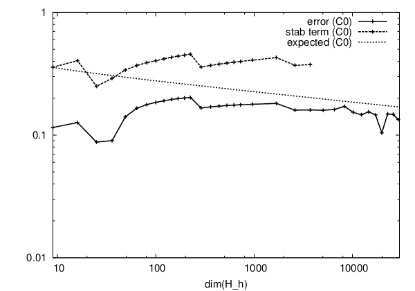
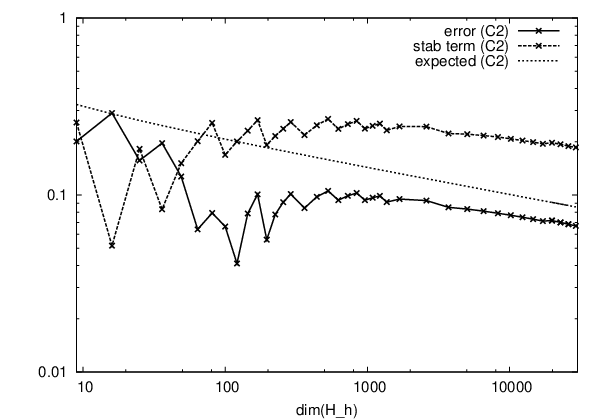
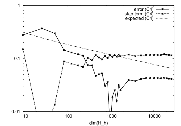
For different values of τ\tau, we present the approximated errors on double logarithmic scales along with the expected convergence rates (upper limit) according to (3.4). For comparability we use the same scales in all the figures. Table 7.1 lists the values of τ\tau with corresponding figure number, data (regularity C2​mC^{2m} and polynomial degrees as mentioned before) and the limit 1/2​(1−1/τ)1/2(1-1/\tau) for the expected convergence rates.

τ\tau figure no. regularity polynomial degree exp. conv. rate 12​(1−1τ)\frac{1}{2}(1-\frac{1}{\tau})
3/23/2 7.2 C0C^{0} 22 1/61/6
5/25/2 7.3 C2C^{2} 55 3/103/10
7/27/2 7.4 C4C^{4} 88 5/145/14
Table 7.1: Values of τ\tau in the numerical experiments with corresponding data, expected convergence rates and figures.

Figures 7.2–7.4 confirm quite precisely the predicted convergence. The lines indicated by “error” give the approximate relative errors calculated by (7.1) whereas the lines “stab term” give the values of the stability term δ⁡(ϵ,t,k,r)​|ψ|Ht​(ΓkcCLOSE\delta(\epsilon,t,k,r)|\psi|_{H^{t}({\Gamma^{c}_{k}}} for ϵ=0\epsilon=0, t=1t=1 (the limit of the regularity) and ψ\psi the calculated RBF approximation, cf. (6.1). The lines “expected” plot the expected convergence rates as listed in Table 7.1. They correspond to our conclusion (6.6) for ϵ=0\epsilon=0 and t=1t=1. All results indicate that the errors have the predicted convergence rates and that the stability term (6.1) fulfills our conjecture (6.2).

We have implemented the method by numerical integration with an overkill of number of integration nodes. We used transformation to polar coordinates so that the singularity from the fundamental solution cancels in the diagonal entries of the stiffness matrix. Nevertheless, note that the polynomial degrees for larger values of τ\tau are large (88 in the case τ=72\tau=\frac{7}{2}) which makes their implementation a non-trivial task.

In the case τ=72\tau=\frac{7}{2} there is a large pre-asymptotic range (Figure 7.4). Note also that for τ=32\tau=\frac{3}{2} we were not able to calculate the stability term for the whole range of unknowns (about 30,000). In this case the radial basis functions are only continuous and the numerical calculation of the H1H^{1}-semi-norm becomes unstable.

Refer to caption
Figure 7.2: Relative error and theoretical convergence rate for τ=1.5\tau=1.5.
Refer to caption
Figure 7.3: Relative error and theoretical convergence rate for τ=2.5\tau=2.5.
Refer to caption
Figure 7.4: Relative error and theoretical convergence rate for τ=3.5\tau=3.5.

Acknowledgment. A significant part of this work has been done while N.H. was visiting the School of Mathematics at The University of New South Wales in Sydney. Their hospitality is gratefully acknowledged.

References

  • [1] R. Arcangéli and M.C.L. de Silanes and J.J. Torrens, An extension of a bound for functions in Sobolev spaces, with applications to (m,s)(m,s)-spline interpolation and smoothing, Numer. Math., 107 (2007), pp. 181–211.
  • [2] J. Bergh and J. Löfström, Interpolation Spaces, no. 223 in Grundlehren der mathematischen Wissenschaften, Springer-Verlag, Berlin, 1976.
  • [3] A. Bespalov and N. Heuer, The pp-version of the boundary element method for hypersingular operators on piecewise plane open surfaces, Numer. Math., 100 (2005), pp. 185–209.
  • [4] A. Bespalov and N. Heuer, The h​php-version of the boundary element method with quasi-uniform meshes in three dimensions, ESAIM Math. Model. Numer. Anal., 42 (2008), pp. 821–849.
  • [5]  , A new 𝐇⁡(div)\mathbf{H}({\rm div})-conforming pp-interpolation operator in two dimensions, ESAIM Math. Model. Numer. Anal., 45 (2011), pp. 255–275.
  • [6] S. C. Brenner and L. R. Scott, The Mathematical Theory of Finite Element Methods, no. 15 in Texts in Applied Mathematics, Springer-Verlag, New York, 1994.
  • [7] M. D. Buhmann, Radial basis functions: theory and implementations, vol. 12 of Cambridge Monographs on Applied and Computational Mathematics, Cambridge University Press, Cambridge, 2003.
  • [8] J. Duchon, Sur l’erreur d’interpolation des fonctions de plusieurs variables par les DmD^{m}-splines, RAIRO Anal. Numér., 12 (1978), pp. 325–334, vi.
  • [9] V. J. Ervin, N. Heuer, and E. P. Stephan, On the hh-pp version of the boundary element method for Symm’s integral equation on polygons, Comput. Methods Appl. Mech. Engrg., 110 (1993), pp. 25–38.
  • [10] G. N. Gatica, M. Healey, and N. Heuer, The boundary element method with Lagrangian multipliers, Numer. Methods Partial Differential Eq., 25 (2009), pp. 1303–1319.
  • [11] P. Grisvard, Elliptic Problems in Nonsmooth Domains, Pitman Publishing Inc., Boston, 1985.
  • [12] M. Healey and N. Heuer, Mortar boundary elements, SIAM J. Numer. Anal., 48 (2010), pp. 1395–1418.
  • [13] N. Heuer, Additive Schwarz method for the pp-version of the boundary element method for the single layer potential operator on aplane screen, Numer. Math., 88 (2001), pp. 485–511.
  • [14] N. Heuer and F.-J. Sayas, Crouzeix–Raviart boundary elements, Numer. Math., 112 (2009), pp. 381–401.
  • [15] J.-L. Lions and E. Magenes, Non-Homogeneous Boundary Value Problems and Applications I, Springer-Verlag, New York, 1972.
  • [16] W. McLean, Strongly Elliptic Systems and Boundary Integral Equations, Cambridge University Press, 2000.
  • [17] F. J. Narcowich and J. D. Ward, Scattered-data interpolation on IRn\mbox{\rm I\kern-1.79993ptR}^{n}: error estimates for radial basis and band-limited functions, SIAM J. Numer. Anal., 36 (2004), pp. 284–300.
  • [18] F. J. Narcowich, J. D. Ward, and H. Wendland, Sobolev bounds on functions with scattered zeros, with applications to radial basis function surface fitting, Math. Comp., 74 (2005), pp. 743–763.
  • [19] T. D. Pham and T. Tran, Solutions to pseudodifferential equations using spherical radial basis functions, Bull. Aust. Math. Soc., 79 (2009), pp. 473–485.
  • [20] T. D. Pham, T. Tran, and Q. T. Le Gia, Numerical solutions to a boundary integral equation with spherical radial basis functions, ANZIAM J., 50 (2008), pp. C266–C281.
  • [21] M. J. D. Powell, The theory of radial basis function approximation in 1990, in Advances in numerical analysis, Vol. II (Lancaster, 1990), Oxford Sci. Publ., Oxford Univ. Press, New York, 1992, pp. 105–210.
  • [22] R. Schaback, A unified theory of radial basis functions. Native Hilbert spaces for radial basis functions. II, J. Comput. Appl. Math., 121 (2000), pp. 165–177. Numerical analysis in the 20th century, Vol. I, Approximation theory.
  • [23] E. M. Stein, Singular Integrals and Differentiability Properties of Functions, Princeton University Press, Princeton, N.J., 1970.
  • [24] E. P. Stephan, Boundary integral equations for screen problems in IR3\mbox{\rm I\kern-1.79993ptR}^{3}, Integral Equations Operator Theory, 10 (1987), pp. 257–263.
  • [25] T. Tran, Q. T. Le Gia, I. H. Sloan, and E. P. Stephan, Boundary integral equations on the sphere with radial basis functions: error analysis, Appl. Numer. Math., 59 (2009), pp. 2857–2871.
  • [26]  , Preconditioners for pseudodifferential equations on the sphere with radial basis functions, Numer. Math., 115 (2010), pp. 141–163.
  • [27] T. von Petersdorff and E. P. Stephan, Decompositions in edge and corner singularities for the solution of the Dirichlet problem of the Laplacian in a polyhedron, Math. Nachr., 149 (1990), pp. 71–104.
  • [28] H. Wendland, Error estimates for interpolation by compactly supported radial basis functions of minimal degree, J. Approx. Theory, 93 (1998), pp. 258–272.
  • [29] H. Wendland, Meshless Galerkin methods using radial basis functions, Math. Comp., 68 (1999), pp. 1521–1531.
  • [30]  , Scattered data approximation, vol. 17 of Cambridge Monographs on Applied and Computational Mathematics, Cambridge University Press, Cambridge, 2005.
  • [31] H. Wendland, Multiscale analysis in Sobolev spaces on bounded domains, Numer. Math., 116 (2010), pp. 493–517.