跳到论文正文
W Papers独立论文阅读器 arXiv:1203.2686 论文正文 计算阅读时间 · 0%
引用这篇论文根据当前论文元数据生成,正式投稿前建议核对。


License: arXiv.org perpetual non-exclusive license
arXiv:1203.2686v1 [math.QA] 13 Mar 2012

A nondiagrammatic description of the Connes-Kreimer Hopf algebra

Alastair Hamilton Address: Department of Mathematics and Statistics, Texas Tech University, Lubbock, TX 79409-1042. USA. Email address: alastair.hamilton@ttu.edu
Abstract.

We demonstrate that the fundamental algebraic structure underlying the Connes-Kreimer Hopf algebra – the insertion pre-Lie structure on graphs – corresponds directly to the canonical pre-Lie structure of polynomial vector fields. Using this fact, we construct a Hopf algebra built from tensors that is isomorphic to a version of the Connes-Kreimer Hopf algebra that first appeared in the perturbative renormalization of quantum field theories.

Key words and phrases: 
Renormalization, Hopf algebra, graph, pre-Lie algebra, invariant theory, BPHZ algorithm
2010 Mathematics Subject Classification
16T05, 16T30, 17B35, 17B66, 81T15, 81T18

1. Introduction

1.1. Background

In this paper we provide a nondiagrammatic description of the Connes-Kreimer Hopf algebra introduced in [CK00] that underlies the perturbative renormalization of quantum field theories. This Hopf algebra was constructed by Connes and Kreimer through the use of a certain fundamental algebraic structure on graphs [CK02]; a pre-Lie structure in which the pre-Lie bracket of two graphs is described by inserting one graph into the other. The Connes-Kreimer Hopf algebra is then realized as the universal enveloping algebra of the resulting Lie algebra. Connes and Kreimer demonstrated that their Hopf algebra encoded the complicated graphical combinatorics present in the BPHZ renormalization algorithm [BP57], [He66], [Zi69]; in that the Feynman amplitudes of the corresponding field theory were realized as a loop of characters in the Hopf algebra and the renormalized values of these Feynman amplitudes were obtained through the Birkhoff factorization of this loop.

We should be careful to explain what we mean by a nondiagrammatic description of this Hopf algebra, as one may consider Connes and Kreimer’s original description to be nondiagrammatic in the sense that it formulated the problem of renormalization through the Birkhoff factorization. Here we are referring to the fact that the Connes-Kreimer Hopf algebra is constructed from combinatorial objects, namely graphs. In this paper we construct a Hopf algebra which is isomorphic to a version of the Connes-Kreimer Hopf algebra and that is built from tensors rather than graphs. Here we draw upon the work of Kontsevich [Ko93] in which he showed how to describe graph complexes in terms of tensors using the invariant theory of the symplectic linear group. Using this correspondence, we demonstrate that the insertion pre-Lie structure on graphs corresponds directly to the canonical pre-Lie structure on polynomial vector fields. This fact is then used to construct our Hopf algebra.

Let us take a moment to point out some distinctions between the algebraic structures that we consider in this paper and those considered in [CK00]. Firstly, the most significant distinction is that our graphs are not decorated by external parameters such as space-time points or momenta. This is not so much because these structures are incompatible with the mathematical framework that we present here, but rather because including them reduces the level of generality that we work in and introduces another level of technicalities. Such decorations will in general depend on the quantum field theory that one is considering, whereas here we prefer to focus simply on the underlying algebraic structures. In [CK00] Connes and Kreimer construct their Hopf algebra for ϕ3\phi^{3} theory in six dimensions, although they point out that their results can be extended to any renormalizable quantum field theory. In some sense, it would be nice to have some universal Hopf algebra whose graphs are not decorated by external parameters, whereby the external parameters appear for any quantum field theory as part of the representation of the Hopf algebra, and in which the problem of renormalization is formulated through the factorization of characters as above. However, the formula (cf. Equation (6) of [CK00]) for the diagonal of the Connes-Kreimer Hopf algebra seems to twist the graphs and their external structures together, making this proposal appear nontrivial to realize. If it were not for this fact, the difference between graphs with or without external parameters would not be material.

Secondly, the Hopf algebra we consider here is generated by all graphs and not just those that are one particle irreducible. This is due to the fact that there seems to be no a priori way to pick out one particle irreducible graphs in our mathematical framework of tensors. This distinction however is not material to the subject of renormalization. The reason for only considering one particle irreducible graphs is that they are the only graphs that require counterterms (cf. Equation (5.5.3) of [Co84]). One may just as easily formulate the BPHZ renormalization algorithm for all graphs, cf. [Co84, §5.3].

Finally, as mentioned above, in this paper we concern ourselves only with the description of the algebraic structures involved and not with the concomitant matters regarding the renormalization of certain quantum field theories. Partly, this is because we prefer to focus on the connection between the insertion pre-Lie structure on graphs and the canonical pre-Lie structure of polynomial vector fields. Partly, it is also because, for the reasons outlined above, making this connection is not completely straightforward. It is known [Co84, §5.6], [Cl11] that one may formulate the process of renormalization without resorting to the graphical combinatorics of the BPHZ algorithm. In these settings, counterterms are computed iteratively and subtracted from the overall Lagrangian. One might hope that the nondiagrammatic descriptions of the algebraic structures of Connes and Kreimer that we provide here may provide a way to bring their methods and ideas to this setting.

Throughout the paper we work with formal objects. For example, our tendency is to work with algebras of power series rather than polynomials. This tendency arises due to the way in which the Connes-Kreimer Hopf algebra is constructed as the dual of a commutative noncocommutative Hopf algebra. This leads to the consideration of objects which have a natural inverse limit structure and a corresponding topology. In this sense, we often consider Hopf algebras in the category of profinite vector spaces, which are a formally complete version of ordinary Hopf algebras and are in one-to-one correspondence with them in the sense that one notion is dual to the other. This distinction causes few real problems beyond some irritating technicalities concerning the convergence of certain expressions involving infinite summations, however it may be unfamiliar to some readers. Consequently, we provide a brief description of the necessary background in Section 1.2 that follows.

The breakdown of the paper is as follows. In Section 2 we recall the original description [CK00] of the Connes-Kreimer Hopf algebra in terms of graphs and describe how, by virtue of a Milnor-Moore type theorem, this Hopf algebra may be described in terms of a pre-Lie structure on connected graphs in which one graph is inserted into another. In Section 3 we proceed to give a nondiagrammatic description of this Hopf algebra. Here the invariant theory of the orthogonal groups plays a crucial role in allowing us to pass from one setting to another. It is in this section that we formulate and prove our main theorem describing the insertion pre-Lie structure of Connes and Kreimer in terms of the canonical pre-Lie structure on polynomial vector fields.

1.2. Notation and conventions

A vector space VV is profinite if it is an inverse limit

V=lim←α∈ℐ⁡VαV=\varprojlim_{\alpha\in\mathcal{I}}V_{\alpha}

of finite-dimensional vector spaces VαV_{\alpha}. The presentation of VV as an inverse limit induces the inverse limit topology upon VV. Profinite vector spaces form a category 𝒫​Vect\mathcal{P}\mathrm{Vect} in which the morphisms are continuous linear maps. This category is anti-equivalent to the usual category of all vector spaces under the functors

(1.1) Vect⇌𝒫​VectV⇀V∗W†↽W\begin{array}[]{ccc}\mathrm{Vect}&\rightleftharpoons&\mathcal{P}\mathrm{Vect}\\ V&\rightharpoonup&V^{*}\\ W^{{\dagger}}&\leftharpoondown&W\end{array}

where V∗V^{*} denotes the linear dual of VV and W†W^{{\dagger}} denotes the continuous linear dual of WW.

If V=lim←α∈ℐ⁡VαV=\varprojlim_{\alpha\in\mathcal{I}}V_{\alpha} and U=lim←β∈𝒥⁡UβU=\varprojlim_{\beta\in\mathcal{J}}U_{\beta} are two profinite vector spaces, we define their completed tensor product ⊗^\hat{\otimes} by

V​⊗^​U:=lim←α,β∈ℐ×𝒥⁡Vα⊗Uβ.V\hat{\otimes}U:=\varprojlim_{\alpha,\beta\in\mathcal{I}\times\mathcal{J}}V_{\alpha}\otimes U_{\beta}.

This construction is functorial in VV and UU. There is a canonical map

(1.2) V⊗U↪V​⊗^​UV\otimes U\hookrightarrow V\hat{\otimes}U

defined by the universal property of inverse limits, whose image is dense in V​⊗^​UV\hat{\otimes}U.

The equivalence (1.1) of categories identifies the tensor product ⊗\otimes in Vect\mathrm{Vect} with the completed tensor product ⊗^\hat{\otimes} in 𝒫​Vect\mathcal{P}\mathrm{Vect} and vice versa. Hence a monoid in one category is the same thing as a comonoid in the other category. We use this perspective tacitly throughout the paper. In particular, if XX is a Hopf algebra in the usual sense, then its dual X∗X^{*} is a Hopf algebra in the category of profinite vector spaces. Conversely, if YY is a Hopf algebra in the category of profinite vector spaces, then its continuous dual Y†Y^{{\dagger}} is a Hopf algebra in the usual sense. Furthermore, one may show that just as ∗\ast turns direct sums into direct products, †{\dagger} turns direct products into direct sums. Similarly, just as ⊗\otimes is distributive with respect to direct sums, the completed tensor product ⊗^\hat{\otimes} is distributive with respect to direct products.

Given a profinite vector space VV, we define the completed tensor algebra of VV by

T^​(V):=∏n=0∞V⊗^​n.\widehat{T}(V):=\prod_{n=0}^{\infty}V^{\hat{\otimes}n}.

Likewise, we define the completed symmetric algebra of VV by

S^​(V):=∏n=0∞V⊗^​n/𝕊n,\widehat{S}(V):=\prod_{n=0}^{\infty}V^{\hat{\otimes}n}/\mathbb{S}_{n},

where the 𝕊n\mathbb{S}_{n} action is the unique action that continuously extends the usual action of 𝕊n\mathbb{S}_{n} on V⊗nV^{\otimes n}. Just as the usual tensor and symmetric algebras have the structure of Hopf algebras, the completed tensor and symmetric algebras have the structure of cocommutative Hopf algebras in the category of profinite vector spaces; that is to say we have maps

μ^:T^​(V)​⊗^​T^​(V)→T^​(V)∇^:T^​(V)→T^​(V)​⊗^​T^​(V)S^:T^​(V)→T^​(V)\begin{split}\hat{\mu}:&\widehat{T}(V)\hat{\otimes}\widehat{T}(V)\to\widehat{T}(V)\\ \hat{\nabla}:&\widehat{T}(V)\to\widehat{T}(V)\hat{\otimes}\widehat{T}(V)\\ \hat{S}:&\widehat{T}(V)\to\widehat{T}(V)\end{split}

which are the unique continuous extensions of the usual maps that make T⁡(V)T(V) into a Hopf algebra, and likewise for the symmetric algebra S^​(V)\widehat{S}(V).

Suppose that we have the structure of a Lie algebra

[−,−]:𝔤​⊗^​𝔤→𝔤[-,-]:\mathfrak{g}\hat{\otimes}\mathfrak{g}\to\mathfrak{g}

on a profinite vector space 𝔤\mathfrak{g}. We define the completed universal enveloping algebra U^​(𝔤)\widehat{U}(\mathfrak{g}) of 𝔤\mathfrak{g} as the quotient of the tensor algebra T^​(𝔤)\widehat{T}(\mathfrak{g}) by the closure of the subspace generated by the usual relations defining U⁡(𝔤)U(\mathfrak{g}). It is straightforward to check that the Hopf algebra structure defined above on T^​(𝔤)\widehat{T}(\mathfrak{g}) descends to the completed universal enveloping algebra U^​(𝔤)\widehat{U}(\mathfrak{g}).

Throughout the paper we work over a ground field 𝕂\mathbb{K} of characteristic zero. For every positive integer nn, there is a canonical vector space Vn:=𝕂nV_{n}:=\mathbb{K}^{n} of dimension nn equipped with a nondegenerate symmetric bilinear form. If x1,…,xnx_{1},\ldots,x_{n} is the standard basis of VnV_{n}, then

(1.3) ⟨xi,xj⟩:={1,i=j0,i≠j}.\langle x_{i},x_{j}\rangle:=\left\{\begin{array}[]{ll}1,&i=j\\ 0,&i\neq j\end{array}\right\}.

If VV is a vector space with a symmetric nondegenerate bilinear form ⟨−,−⟩\langle-,-\rangle, then we denote the group of endomorphisms ϕ\phi of VV satisfying

⟨ϕ⁡(v),ϕ⁡(w)⟩=⟨v,w⟩, for all ​v,w∈V\langle\phi(v),\phi(w)\rangle=\langle v,w\rangle,\text{ for all }v,w\in V

by O⁡(V)O(V). Such transformations will be referred to as orthogonal transformations. In particular, we will denote O⁡(Vn)O(V_{n}) by O⁡(n)O(n).

Given a symmetric bilinear form ⟨−,−⟩\langle-,-\rangle on a vector space VV, the inverse form ⟨−,−⟩−1\langle-,-\rangle^{-1} on V∗V^{*} is defined by the following commutative diagram;

𝕂\textstyle{\mathbb{K}}V⊗V\textstyle{V\otimes V\ignorespaces\ignorespaces\ignorespaces\ignorespaces\ignorespaces\ignorespaces\ignorespaces\ignorespaces}⟨−,−⟩\scriptstyle{\langle-,-\rangle}D⊗D\scriptstyle{D\otimes D}V∗⊗V∗\textstyle{V^{*}\otimes V^{*}\ignorespaces\ignorespaces\ignorespaces\ignorespaces}⟨−,−⟩−1\scriptstyle{\langle-,-\rangle^{-1}}

where D(v):=[x↦⟨v,x⟩]D(v):=[x\mapsto\langle v,x\rangle].

2. The Connes-Kreimer Hopf algebra and its graphical description

In this section we recall the graphical description of the Connes-Kreimer Hopf algebra as it was outlined in [CK00]. We begin by introducing the elementary objects, namely graphs, that it is constructed from and describe some elementary operations on them. We then proceed to a description of the Connes-Kreimer Hopf algebra and its primitive elements. After formulating a Milnor-Moore type theorem for this Hopf algebra, we recall the fundamental insertion pre-Lie structure on graphs defined in [CK00] and [CK02] that describes the Lie algebra structure of its primitive elements.

2.1. Graphs

We start by introducing elementary definitions of the notion of graph and subgraph and describe how to collapse a subgraph of a graph to a point.

Definition 2.1.

A graph Γ\Gamma is a set Γ\Gamma consisting of the half-edges of the graph together with the data of:

  1. (1)

    A partition E⁡(Γ)E(\Gamma) of Γ\Gamma into pairs, called the set of edges of Γ\Gamma.

  2. (2)

    A partition V⁡(Γ)V(\Gamma) of Γ\Gamma, called the set of vertices of Γ\Gamma. The cardinality of a vertex v∈V⁡(Γ)v\in V(\Gamma) is called its valency. Vertices may have any valency.

  3. (3)

    A subset Vext​(Γ)V_{\mathrm{ext}}(\Gamma) of the 1-valent vertices of Γ\Gamma, called the external vertices.

Refer to caption
Figure 1. Here, the external vertices are denoted by white dots and the external edges are denoted by dashed lines. Internal vertices are denoted by solid dots and internal edges are denoted by solid lines.

Any vertex which is not an external vertex is called an internal vertex. The set of internal vertices of Γ\Gamma will be denoted by Vint​(Γ)V_{\mathrm{int}}(\Gamma). An edge will be called external if it is connected to an external vertex; otherwise, it will be called internal. The set of external edges will be denoted by Eext​(Γ)E_{\mathrm{ext}}(\Gamma) and the set of internal edges will be denoted by Eint​(Γ)E_{\mathrm{int}}(\Gamma). The empty graph is considered to be a graph and denoted by 𝟏\mathbf{1}. We say that two graphs are isomorphic if there is a bijective mapping of the half-edges from one to the other preserving structures (1) to (3) above.

We may contract any internal edge of a graph Γ\Gamma.

Definition 2.2.

Let e={h1,h2}e=\{h_{1},h_{2}\} be an internal edge of a graph Γ\Gamma. We define Γ/e\Gamma/e to be the result of contracting the edge ee in Γ\Gamma. Specifically:

  1. (1)
    E⁡(Γ/e)=E⁡(Γ)−{e}.E(\Gamma/e)=E(\Gamma)-\{e\}.
  2. (2)
    1. (a)

      If ee is not a loop and hence is incident to two vertices

      v1={h1,x1,…,xk}andv2={h2,y1,…,yl}v_{1}=\{h_{1},x_{1},\ldots,x_{k}\}\quad\text{and}\quad v_{2}=\{h_{2},y_{1},\ldots,y_{l}\}

      then the vertices of Γ/e\Gamma/e consist of all the other vertices of Γ\Gamma together with a new vertex

      v={x1,…,xk,y1,…,yl}v=\{x_{1},\ldots,x_{k},y_{1},\ldots,y_{l}\}

      formed by combining v1v_{1} and v2v_{2}.

    2. (b)

      If ee is a loop incident to a vertex

      v={h1,h2,x1,…,xk}v=\{h_{1},h_{2},x_{1},\ldots,x_{k}\}

      then the vertices of Γ/e\Gamma/e consist of all the other vertices of Γ\Gamma together with the new vertex

      v′={x1,…,xk}v^{\prime}=\{x_{1},\ldots,x_{k}\}

      formed by removing the loop ee.

  3. (3)

    The external vertices of Γ/e\Gamma/e are the same as those of Γ\Gamma.

Refer to caption
Figure 2. Contracting edges and loops in a graph.
Remark 2.3.

Note that one may check that it does not matter what order one contracts edges in a graph, that is to say that

(Γ/e1)/e2=(Γ/e2)/e1(\Gamma/e_{1})/e_{2}=(\Gamma/e_{2})/e_{1}

for any two internal edges e1e_{1} and e2e_{2}.

Definition 2.4.

A subgraph γ\gamma of a graph Γ\Gamma is a subset of the internal edges Eint​(Γ)E_{\mathrm{int}}(\Gamma) of Γ\Gamma. By Remark 2.3, we may associate to any subgraph γ={e1,…,en}\gamma=\{e_{1},\ldots,e_{n}\} of Γ\Gamma the graph

Γ/γ:=(…​((Γ/e1)/e2)​…/en)\Gamma/\gamma:=(\ldots((\Gamma/e_{1})/e_{2})\ldots/e_{n})

with all the edges of γ\gamma contracted.

To any subgraph γ={e1,…,en}\gamma=\{e_{1},\ldots,e_{n}\} of Γ\Gamma, we may associate a graph in the sense of Definition 2.1, which, by an abuse of notation, we shall also denote by γ\gamma. It is constructed as follows. Let

{v∈V(Γ):v∩(∪i=1nei)≠ϕ}={v1,…,vr}\{v\in V(\Gamma):v\cap\left(\cup_{i=1}^{n}e_{i}\right)\neq\phi\}=\{v_{1},\ldots,v_{r}\}

be a list of those vertices which intersect the subgraph γ\gamma and consider the set

H=⋃i=1rviH=\bigcup_{i=1}^{r}v_{i}

of half-edges of Γ\Gamma formed by their union. Let h1,…,hkh_{1},\ldots,h_{k} be a list of those half-edges in HH which do not belong to any edge eie_{i} of γ\gamma;

H−⋃i=1nei={h1,…,hk}.H-\bigcup_{i=1}^{n}e_{i}=\{h_{1},\ldots,h_{k}\}.

These half-edges will form the ends of the external edges of γ\gamma. To this end we introduce another disjoint set of half-edges h1′,…,hk′h^{\prime}_{1},\ldots,h^{\prime}_{k} to form the other ends of these external edges. The graph γ\gamma may now be defined as follows:

Refer to caption
Figure 3. Constructions associated to subgraphs.
  1. (1)

    The half-edges of γ\gamma consist of H∪{h1′,…,hk′}H\cup\{h^{\prime}_{1},\ldots,h^{\prime}_{k}\}.

  2. (2)

    The edges of γ\gamma are

    E⁡(γ)={e1,…,en,{h1,h1′},…​{hk,hk′}}.E(\gamma)=\{e_{1},\ldots,e_{n},\{h_{1},h^{\prime}_{1}\},\ldots\{h_{k},h^{\prime}_{k}\}\}.
  3. (3)

    The vertices of γ\gamma are

    V⁡(γ)={v1,…,vr,{h1′},…,{hk′}}.V(\gamma)=\{v_{1},\ldots,v_{r},\{h^{\prime}_{1}\},\ldots,\{h^{\prime}_{k}\}\}.

    The external vertices of γ\gamma are Vext​(γ)={{h1′},…,{hk′}}V_{\mathrm{ext}}(\gamma)=\{\{h^{\prime}_{1}\},\ldots,\{h^{\prime}_{k}\}\}.

2.2. The Connes-Kreimer Hopf algebra

Now that we have introduced some of the elementary objects, we are in a position to begin recalling the definition of the Connes-Kreimer Hopf algebra. We begin by describing a simple commutative algebra structure on graphs.

Definition 2.5.

Let ℋ\mathcal{H} be the vector space freely generated by isomorphism classes of graphs. Given two graphs Γ1\Gamma_{1} and Γ2\Gamma_{2} we may form their disjoint union Γ1⊔Γ2\Gamma_{1}\sqcup\Gamma_{2}. This gives ℋ\mathcal{H} the structure of an algebra, with multiplication μ\mu given by disjoint union. We will denote the subspace of ℋ\mathcal{H} generated by connected graphs by ℋc\mathcal{H}_{c}. Note that the empty graph is not considered to be connected. The spaces ℋ\mathcal{H} and ℋc\mathcal{H}_{c} posses natural gradings

ℋ=⨁n=0∞ℋnℋc=⨁n=0∞ℋc,n\mathcal{H}=\bigoplus_{n=0}^{\infty}\mathcal{H}_{n}\qquad\mathcal{H}_{c}=\bigoplus_{n=0}^{\infty}\mathcal{H}_{c,n}

where ℋn\mathcal{H}_{n} and ℋc,n\mathcal{H}_{c,n} are those subspaces of ℋ\mathcal{H} and ℋc\mathcal{H}_{c} respectively which are generated by graphs with precisely nn edges. These gradings are of finite-type in that each of the subspaces ℋn\mathcal{H}_{n} and ℋc,n\mathcal{H}_{c,n} are finite-dimensional.

Occasionally, we will wish to use a finer grading than the one above. We may write

(2.1) ℋ=⨁n,m,k=0∞ℋn,m,kℋc=⨁n,m,k=0∞ℋc;n,m,k\mathcal{H}=\bigoplus_{n,m,k=0}^{\infty}\mathcal{H}_{n,m,k}\qquad\mathcal{H}_{c}=\bigoplus_{n,m,k=0}^{\infty}\mathcal{H}_{c;n,m,k}

where both ℋn,m,k\mathcal{H}_{n,m,k} and ℋc;n,m,k\mathcal{H}_{c;n,m,k} are spanned by graphs with precisely nn edges, mm internal edges and kk external vertices. The subscript ≥a\geq a will be used to denote the subspace spanned by elements of degree greater than or equal to aa, for instance

ℋ∙,≥a,∙:=⨁n,k=0m=a∞ℋn,m,k\mathcal{H}_{\bullet,\geq a,\bullet}:=\bigoplus_{\begin{subarray}{c}n,k=0\\ m=a\end{subarray}}^{\infty}\mathcal{H}_{n,m,k}

will denote the subspace of ℋ\mathcal{H} spanned by graphs with at least aa internal edges.

Proposition 2.6.

ℋ\mathcal{H} is a polynomial algebra over the subspace of connected graphs, that is to say we have the following canonical isomorphism of algebras;

S⁡(ℋc)≅ℋΓ1⊗⋯⊗Γk↦Γ1⊔⋯⊔Γk\begin{array}[]{ccc}S(\mathcal{H}_{c})&\cong&\mathcal{H}\\ \Gamma_{1}\otimes\cdots\otimes\Gamma_{k}&\mapsto&\Gamma_{1}\sqcup\cdots\sqcup\Gamma_{k}\end{array}
Proof.

This follows from the fact that any graph is the disjoint union of its connected components. ∎

Remark 2.7.

Since S⁡(ℋc)S(\mathcal{H}_{c}) has a canonical cocommutative comultiplication on it in which the subspace ℋc\mathcal{H}_{c} coincides with the space of primitive elements, the above theorem also endows ℋ\mathcal{H} with a corresponding cocommutative comultiplication. This comultiplication differs from the noncocommutative comultiplication of Connes and Kreimer that we will introduce later in Definition 2.11.

The Connes-Kreimer Hopf algebra will be constructed as the dual of ℋ\mathcal{H}. To assist us in describing it, we introduce a nondegenerate bilinear form on graphs. Since ℋ\mathcal{H} has a preferred basis consisting of isomorphism classes of graphs, this allows us to define a symmetric bilinear form on ℋ\mathcal{H} as follows.

Definition 2.8.

Given two graphs Γ1\Gamma_{1} and Γ2\Gamma_{2} we define

(2.2) ⟨Γ1,Γ2⟩={1,Γ1≅Γ20,Γ1≇Γ2}.\langle\Gamma_{1},\Gamma_{2}\rangle=\left\{\begin{array}[]{rl}1,&\Gamma_{1}\cong\Gamma_{2}\\ 0,&\Gamma_{1}\ncong\Gamma_{2}\end{array}\right\}.

This defines a symmetric bilinear form on ℋ\mathcal{H} which is nondegenerate in the sense that it is nondegenerate on each ℋn\mathcal{H}_{n}. Obviously the pairing is trivial in the event that Γ1\Gamma_{1} and Γ2\Gamma_{2} have a different number of edges so that ℋi\mathcal{H}_{i} and ℋj\mathcal{H}_{j} are orthogonal if i≠ji\neq j.

Definition 2.9.

Let us denote by ℋ^\widehat{\mathcal{H}} the vector space freely generated by formal infinite linear combinations of isomorphism classes of graphs. This space has the same natural grading as ℋ\mathcal{H};

ℋ^=∏n=0∞ℋn.\widehat{\mathcal{H}}=\prod_{n=0}^{\infty}\mathcal{H}_{n}.

As before, we have the identification ℋ^≅S^​(ℋ^c)\widehat{\mathcal{H}}\cong\widehat{S}(\widehat{\mathcal{H}}_{c}) of Proposition 2.6. The bilinear form (2.2) defined in Definition 2.8 yields the following simple proposition describing this space as the space that is dual to ℋ\mathcal{H}.

Proposition 2.10.

There is a canonical isomorphism between ℋ^\widehat{\mathcal{H}} and ℋ∗\mathcal{H}^{*} given by

(2.3) ℋ^=∏n=0∞ℋn≅∏n=0∞ℋn∗=ℋ∗Γ↦|Aut⁡(Γ)|​⟨Γ,−⟩\begin{array}[]{rcl}\widehat{\mathcal{H}}=\prod_{n=0}^{\infty}\mathcal{H}_{n}&\cong&\prod_{n=0}^{\infty}\mathcal{H}_{n}^{*}=\mathcal{H}^{*}\\ \Gamma&\mapsto&|\Aut(\Gamma)|\langle\Gamma,-\rangle\end{array}

□\square

Now we can recall how the Connes-Kreimer coproduct on graphs is defined. This coproduct is the fundamental algebraic structure that encodes the graphical combinatorics of the BPHZ algorithm [CK00].

Definition 2.11.

By Proposition 2.6, in order to define a bialgebra structure on ℋ\mathcal{H}, it is sufficient to specify how the comultiplication

∇:ℋ→ℋ⊗ℋ\nabla:\mathcal{H}\to\mathcal{H}\otimes\mathcal{H}

behaves on connected graphs. This is defined by Connes-Kreimer [CK00] using the following formula;

(2.4) ∇(Γ):=𝟏⊗Γ+Γ⊗𝟏+∑γ⊊Γγ⊗Γ/γ\nabla(\Gamma):=\mathbf{1}\otimes\Gamma+\Gamma\otimes\mathbf{1}+\sum_{\gamma\subsetneq\Gamma}\gamma\otimes\Gamma/\gamma

where the sum is taken over all nontrivial subgraphs of Γ\Gamma.

Remark 2.12.

Note that if Γ∈ℋn\Gamma\in\mathcal{H}_{n}, then ∇(Γ)\nabla(\Gamma) will be an inhomogeneous sum of elements of total degree kk for kk between nn and 3​n3n. However, if we consider the grading on ℋ\mathcal{H} defined by the number of internal edges of a graph, then ∇\nabla will have degree zero in this grading. These facts may be summarized by the identity

∇(ℋn,m,∙)⊂⨁k=n3​n(⨁i1+j1=ki2+j2=mℋi1,i2,∙⊗ℋj1,j2,∙).\nabla(\mathcal{H}_{n,m,\bullet})\subset\bigoplus_{k=n}^{3n}\left(\bigoplus_{\begin{subarray}{c}i_{1}+j_{1}=k\\ i_{2}+j_{2}=m\end{subarray}}\mathcal{H}_{i_{1},i_{2},\bullet}\otimes\mathcal{H}_{j_{1},j_{2},\bullet}\right).

Theorem 1 of [CK00] due to Connes-Kreimer states that this comultiplication is coassociative and gives ℋ\mathcal{H} the structure of a commutative Hopf algebra. The Connes-Kreimer Hopf algebra is then given by taking the linear dual of this Hopf algebra. The bilinear form introduced in Definition 2.8 allows us to describe this dual Hopf algebra in terms of algebraic structures defined on ℋ^\widehat{\mathcal{H}}.

Definition 2.13.

The vector space ℋ^\widehat{\mathcal{H}} may be endowed with the structure of a cocommutative Hopf algebra (in the category 𝒫​Vect\mathcal{P}\mathrm{Vect} of profinite vector spaces) in the following manner. Let I:ℋ^→ℋ∗I:\widehat{\mathcal{H}}\to\mathcal{H}^{*} be the map given by (2.3). The multiplication and comultiplication

⋆:ℋ^​⊗^​ℋ^→ℋ^andΔ:ℋ^→ℋ^​⊗^​ℋ^\star:\widehat{\mathcal{H}}\hat{\otimes}\widehat{\mathcal{H}}\to\widehat{\mathcal{H}}\quad\text{and}\quad\Delta:\widehat{\mathcal{H}}\to\widehat{\mathcal{H}}\hat{\otimes}\widehat{\mathcal{H}}

are defined by the formulae:

I∘⋆=∇∗∘(I​⊗^​I)μ∗∘I=(I​⊗^​I)∘Δ\begin{split}I\circ\star&=\nabla^{*}\circ(I\hat{\otimes}I)\\ \mu^{*}\circ I&=(I\hat{\otimes}I)\circ\Delta\end{split}
Remark 2.14.

It follows from Remark 2.12 that ⋆\star has degree zero in the grading by the number of internal edges. Additionally, if Γ1\Gamma_{1} is a formal sum of elements from ℋk\mathcal{H}_{k} for k≥3​nk\geq 3n then both Γ1⋆Γ2\Gamma_{1}\star\Gamma_{2} and Γ2⋆Γ1\Gamma_{2}\star\Gamma_{1} will be a formal sum of elements from ℋk\mathcal{H}_{k} for k≥nk\geq n. We may summarize this as

(2.5) ⋆([ℋ≥3​n,m1,∙],[ℋ∙,m2,∙])⊂ℋ≥n,m1+m2,∙⋆([ℋ∙,m1,∙],[ℋ≥3​n,m2,∙])⊂ℋ≥n,m1+m2,∙\begin{split}\star\left([\mathcal{H}_{\geq 3n,m_{1},\bullet}],[\mathcal{H}_{\bullet,m_{2},\bullet}]\right)&\subset\mathcal{H}_{\geq n,m_{1}+m_{2},\bullet}\\ \star\left([\mathcal{H}_{\bullet,m_{1},\bullet}],[\mathcal{H}_{\geq 3n,m_{2},\bullet}]\right)&\subset\mathcal{H}_{\geq n,m_{1}+m_{2},\bullet}\end{split}

We begin by determining a more convenient description of the cocommutative comultiplication Δ\Delta. Consider the isomorphism T:S⁡(ℋc)→ℋT:S(\mathcal{H}_{c})\to\mathcal{H} of Proposition 2.6. This induces an isomorphism

T∗:ℋ∗→∏n=0∞[(ℋc∗)⊗^​n]𝕊n.T^{*}:\mathcal{H}^{*}\to\prod_{n=0}^{\infty}\left[(\mathcal{H}_{c}^{*})^{\hat{\otimes}n}\right]^{\mathbb{S}_{n}}.

The latter space of invariants may be identified with the coinvariants S^​(ℋc∗)=∏n=0∞[(ℋc∗)⊗^​n]𝕊n\widehat{S}(\mathcal{H}_{c}^{*})=\prod_{n=0}^{\infty}\left[(\mathcal{H}_{c}^{*})^{\hat{\otimes}n}\right]_{\mathbb{S}_{n}} under the map

ωn:[(ℋc∗)⊗^​n]𝕊n→[(ℋc∗)⊗^​n]𝕊nf↦1n!​f\begin{array}[]{rcl}\omega_{n}:\left[(\mathcal{H}_{c}^{*})^{\hat{\otimes}n}\right]^{\mathbb{S}_{n}}&\to&\left[(\mathcal{H}_{c}^{*})^{\hat{\otimes}n}\right]_{\mathbb{S}_{n}}\\ f&\mapsto&\frac{1}{n!}f\end{array}
Proposition 2.15.

The following diagram of isomorphisms commutes

ℋ^\textstyle{\widehat{\mathcal{H}}\ignorespaces\ignorespaces\ignorespaces\ignorespaces}I\scriptstyle{I}ℋ∗\textstyle{\mathcal{H}^{*}\ignorespaces\ignorespaces\ignorespaces\ignorespaces}ω∘T∗\scriptstyle{\omega\circ T^{*}}S^​(ℋ^c)\textstyle{\widehat{S}(\widehat{\mathcal{H}}_{c})\ignorespaces\ignorespaces\ignorespaces\ignorespaces\ignorespaces\ignorespaces\ignorespaces\ignorespaces}S⁡(I)\scriptstyle{S(I)}T^\scriptstyle{\widehat{T}}S^​(ℋc∗)\textstyle{\widehat{S}(\mathcal{H}_{c}^{*})}
Proof.

The commutativity of the above diagram is equivalent to the following identity

|Aut⁡(Γ1⊔⋯⊔Γn)|​⟨Γ1⊔⋯⊔Γn,γ1⊔⋯⊔γn⟩=∑σ∈𝕊n|Aut(Γ1)|⋯|Aut(Γn)|⟨Γ1,γσ⁡(1)⟩⋯⟨Γn,γσ⁡(n)⟩.|\Aut(\Gamma_{1}\sqcup\cdots\sqcup\Gamma_{n})|\langle\Gamma_{1}\sqcup\cdots\sqcup\Gamma_{n},\gamma_{1}\sqcup\cdots\sqcup\gamma_{n}\rangle=\\ \sum_{\sigma\in\mathbb{S}_{n}}|\Aut(\Gamma_{1})|\cdots|\Aut(\Gamma_{n})|\langle\Gamma_{1},\gamma_{\sigma(1)}\rangle\cdots\langle\Gamma_{n},\gamma_{\sigma(n)}\rangle.

which holds for all connected graphs Γ1,…​Γn,γ1,…,γn\Gamma_{1},\ldots\Gamma_{n},\gamma_{1},\ldots,\gamma_{n}. This identity follows in turn from the decomposition

Aut(Γi1⊔⋯⊔Γin)=[Aut(Γi1)×⋯×Aut(Γin)]⋊{σ∈𝕊n:ir=iσ⁡(r), for all r}\Aut(\Gamma_{i_{1}}\sqcup\cdots\sqcup\Gamma_{i_{n}})=[\Aut(\Gamma_{i_{1}})\times\cdots\times\Aut(\Gamma_{i_{n}})]\rtimes\{\sigma\in\mathbb{S}_{n}:i_{r}=i_{\sigma(r)},\text{ for all }r\}

of Aut⁡(Γi1⊔⋯⊔Γin)\Aut(\Gamma_{i_{1}}\sqcup\cdots\sqcup\Gamma_{i_{n}}) as a wreath product; where Γi,i∈ℐ\Gamma_{i},i\in\mathcal{I} is a complete list of representatives for isomorphism classes of connected graphs. ∎

Remark 2.16.

This proposition affords us a more convenient description of the comultiplication Δ\Delta and consequently allows us to describe the primitive elements of the Hopf algebra (ℋ^,⋆,Δ)(\widehat{\mathcal{H}},\star,\Delta). It is well-known that the isomorphism ω∘T∗\omega\circ T^{*} maps the comultiplication μ∗\mu^{*} on ℋ∗\mathcal{H}^{*} to the canonical cocommutative comultiplication on S^​(ℋc∗)\widehat{S}(\mathcal{H}_{c}^{*}). Consequently, the isomorphism T^:S^​(ℋ^c)→ℋ^\widehat{T}:\widehat{S}(\widehat{\mathcal{H}}_{c})\to\widehat{\mathcal{H}} identifies the comultiplication Δ\Delta on ℋ^\widehat{\mathcal{H}} with the canonical cocommutative comultiplication on S^​(ℋ^c)\widehat{S}(\widehat{\mathcal{H}}_{c}). From this it follows that the subspace of primitive elements of (ℋ^,⋆,Δ)(\widehat{\mathcal{H}},\star,\Delta) coincides with ℋ^c\widehat{\mathcal{H}}_{c}.

2.3. A Milnor-Moore type theorem

The Hopf algebra (ℋ^,⋆,Δ)(\widehat{\mathcal{H}},\star,\Delta) may be described in terms of the universal enveloping algebra of a certain Lie algebra by virtue of a Milnor-Moore type theorem. This will allow us to analyze the algebraic structure of this Hopf algebra by analyzing the underlying structure of this Lie algebra. Our first task is to pick out the relevant subalgebra of (ℋ^,⋆,Δ)(\widehat{\mathcal{H}},\star,\Delta).

The algebra ℋ^\widehat{\mathcal{H}} contains a commutative subalgebra of graphs with no internal edges, which plays no role in the renormalization process and contributes nothing to the algebraic structure. Therefore, we would like to separate this subalgebra out of the discussion. Let

ℋ^c+:=ℋ^c;∙,≥1,∙\widehat{\mathcal{H}}_{c}^{+}:=\widehat{\mathcal{H}}_{c;\bullet,\geq 1,\bullet}

denote the subspace of ℋ^c\widehat{\mathcal{H}}_{c} which is formally spanned by those graphs with at least one internal edge. We shall define ℋ^+≅S^​(ℋ^c+)\widehat{\mathcal{H}}^{+}\cong\widehat{S}(\widehat{\mathcal{H}}_{c}^{+}) to be the corresponding subspace of ℋ^\widehat{\mathcal{H}} which is formally generated by disjoint unions of connected graphs with at least one internal edge.

Proposition 2.17.

The bialgebra (ℋ^,⋆,Δ)(\widehat{\mathcal{H}},\star,\Delta) is the tensor product of a strictly commutative subalgebra KK and the subalgebra ℋ^+\widehat{\mathcal{H}}^{+}

ℋ^≅K​⊗^​ℋ^+.\widehat{\mathcal{H}}\cong K\hat{\otimes}\widehat{\mathcal{H}}^{+}.
Proof.

ℋ^c\widehat{\mathcal{H}}_{c} splits as a direct sum of the subspace I:=ℋ^c;∙0∙I:=\widehat{\mathcal{H}}_{c;\bullet 0\bullet} consisting of graphs which have no internal edges and the subspace ℋ^c+\widehat{\mathcal{H}}_{c}^{+}. Hence

ℋ^≅S^​(ℋ^c)≅S^​(I)​⊗^​S^​(ℋ^c+)=S^​(I)​⊗^​ℋ^+.\widehat{\mathcal{H}}\cong\widehat{S}(\widehat{\mathcal{H}}_{c})\cong\widehat{S}(I)\hat{\otimes}\widehat{S}(\widehat{\mathcal{H}}_{c}^{+})=\widehat{S}(I)\hat{\otimes}\widehat{\mathcal{H}}^{+}.

Set K:=S^​(I)K:=\widehat{S}(I). Since it is impossible for any graph corresponding to a term in the expression (2.4) for the coproduct ∇(Γ)\nabla(\Gamma) to have no internal edges, unless Γ\Gamma itself has no internal edges, it follows that KK is not just a subalgebra of ℋ^\widehat{\mathcal{H}}, but in fact a commutative subalgebra whose multiplication coincides with disjoint union. Furthermore, this fact also implies not only that ℋ^+\widehat{\mathcal{H}}^{+} is a subalgebra of ℋ^\widehat{\mathcal{H}}, but that

Γ1⋆Γ2=Γ1⊔Γ2\Gamma_{1}\star\Gamma_{2}=\Gamma_{1}\sqcup\Gamma_{2}

for all Γ1∈ℋ^+\Gamma_{1}\in\widehat{\mathcal{H}}^{+} and Γ2∈K\Gamma_{2}\in K. Hence we have the following isomorphism;

K​⊗^​ℋ^+≅ℋ^Γ1​⊗^​Γ2↦Γ1⋆Γ2\begin{array}[]{ccc}K\hat{\otimes}\widehat{\mathcal{H}}^{+}&\cong&\widehat{\mathcal{H}}\\ \Gamma_{1}\hat{\otimes}\Gamma_{2}&\mapsto&\Gamma_{1}\star\Gamma_{2}\end{array}

∎

Since ℋ^+≅S^​(ℋ^c+)\widehat{\mathcal{H}}^{+}\cong\widehat{S}(\widehat{\mathcal{H}}_{c}^{+}), this induces another grading on ℋ^+\widehat{\mathcal{H}}^{+} by the order of a polynomial in S^​(ℋ^c+)\widehat{S}(\widehat{\mathcal{H}}_{c}^{+}); or equivalently, the number of connected components of a graph Γ∈ℋ^+\Gamma\in\widehat{\mathcal{H}}^{+}. One can check that by Equation (2.4),

(2.6) Γ1⋆Γ2=Γ1⊔Γ2+terms of order <order⁡(Γ1)+order⁡(Γ2).\Gamma_{1}\star\Gamma_{2}=\Gamma_{1}\sqcup\Gamma_{2}+\text{terms of order }<\mathrm{order}(\Gamma_{1})+\mathrm{order}(\Gamma_{2}).

One consequence of this equation is that ℋ^+\widehat{\mathcal{H}}^{+} is (formally) generated by primitive elements under ⋆\star, and consequently a Milnor-Moore type theorem holds

Theorem 2.18.

The bialgebra (ℋ^+,⋆,Δ)(\widehat{\mathcal{H}}^{+},\star,\Delta) is canonically isomorphic to the (completed) universal enveloping algebra of its primitive elements ℋ^c+\widehat{\mathcal{H}}_{c}^{+};

(2.7) U^​(ℋ^c+)≅ℋ^+Γ1⊗^⋯⊗^Γn↦Γ1⋆⋯⋆Γn\begin{array}[]{ccc}\widehat{U}(\widehat{\mathcal{H}}_{c}^{+})&\cong&\widehat{\mathcal{H}}^{+}\\ \Gamma_{1}\hat{\otimes}\cdots\hat{\otimes}\Gamma_{n}&\mapsto&\Gamma_{1}\star\cdots\star\Gamma_{n}\end{array}
Proof.

The proof involves standard arguments [MM65], but the situation is complicated by the fact that we are working with formal objects and the consequent need to ensure that certain expressions are convergent. Additionally, the situation is made more awkward by the fact that ⋆\star is inhomogeneous in the finite-type grading by number of edges. The reader who feels no uneasiness about working with formal objects may benefit from skipping the details. We include them only for the sake of being thorough.

It follows from Remark 2.14 and Equation (2.5) that the map (2.7) is well-defined, in that those expressions which are implicit in its definition are convergent. More precisely, an element of U^​(ℋ^c+)\widehat{U}(\widehat{\mathcal{H}}_{c}^{+}) is a formal sum of elements on the left-hand side of (2.7) and its image is consequently the corresponding formal sum of elements on the right-hand side of (2.7), which converges in the inverse limit topology by (2.5). For this, it is important that we work with graphs with at least one internal edge.

We start by showing that (2.7) is surjective. Any Λ∈ℋ^+\Lambda\in\widehat{\mathcal{H}}^{+} will be a formal sum

Λ=∑k=1∞Λk\Lambda=\sum_{k=1}^{\infty}\Lambda_{k}

of terms Λk∈ℋk+\Lambda_{k}\in\mathcal{H}_{k}^{+} with kk edges. In turn, each Λk\Lambda_{k} will be a (finite) sum of terms of the form

(2.8) Γ1⊔⋯⊔Γn\Gamma_{1}\sqcup\cdots\sqcup\Gamma_{n}

for n≤kn\leq k, with each Γi∈ℋc+\Gamma_{i}\in\mathcal{H}_{c}^{+}. Consequently, we may write

Λk=∑n=1kΛkn\Lambda_{k}=\sum_{n=1}^{k}\Lambda_{k}^{n}

where Λkn\Lambda_{k}^{n} is a sum of graphs with nn connected components, i.e. a sum of terms of the form (2.8).

By Equation (2.6) and a simple, standard inductive argument, we may show that Λkn\Lambda_{k}^{n} is the image of some Λ~kn∈T⁡(ℋc+)\tilde{\Lambda}_{k}^{n}\in T(\mathcal{H}_{c}^{+}) under the map (2.7), and hence Λk\Lambda_{k} will be the image of

Λ~k:=∑n=1kΛ~kn\tilde{\Lambda}_{k}:=\sum_{n=1}^{k}\tilde{\Lambda}_{k}^{n}

under the map (2.7). I claim that Λ\Lambda is the image of Λ~:=∑k=1∞Λ~k\tilde{\Lambda}:=\sum_{k=1}^{\infty}\tilde{\Lambda}_{k} under (2.7), but for this to be true, we must first prove that this formal sum converges.

Consider the grading that is induced on T⁡(ℋc+)T(\mathcal{H}_{c}^{+}) by the grading on ℋc+\mathcal{H}_{c}^{+} whose degree coincides with the total number of edges in a graph. I claim that if k≥(3​N)Nk\geq(3N)^{N}, then Λ~k\tilde{\Lambda}_{k} will be a sum of terms of degree ≥N\geq N. This will prove that Λ~\tilde{\Lambda} is a convergent sum and establish that (2.7) is surjective.

If we consider for a moment the grading induced upon T⁡(ℋc+)T(\mathcal{H}_{c}^{+}) by the number of internal edges, then if n≥Nn\geq N, (2.8) will have at least NN internal edges, as each Γi\Gamma_{i} has at least one. Since ⋆\star has degree zero in the grading by internal edges, it follows from the construction of Λ~kn\tilde{\Lambda}_{k}^{n} that it will be a sum of terms of degree ≥N\geq N in the grading by internal edges, and hence a sum of terms of degree ≥N\geq N in the grading by the total number of edges.

Hence, we need only consider Λ~kn\tilde{\Lambda}_{k}^{n} for n<Nn<N. If n<Nn<N and the graph (2.8) has k≥(3​N)Nk\geq(3N)^{N} edges, then some connected component Γi\Gamma_{i} must have at least 3N​NN−13^{N}N^{N-1} edges. Hence Γ1⋆⋯⋆Γn∈ℋc,≥(3​N)N−1+\Gamma_{1}\star\cdots\star\Gamma_{n}\in\mathcal{H}_{c,\geq(3N)^{N-1}}^{+} and

Γ1⋆⋯⋆Γn=Γ1⊔⋯⊔Γn+terms of order ≤n−1.\Gamma_{1}\star\cdots\star\Gamma_{n}=\Gamma_{1}\sqcup\cdots\sqcup\Gamma_{n}+\text{terms of order }\leq n-1.

Proceeding by induction to eliminate, in the same manner, terms of lower and lower order; we may conclude that Λkn\Lambda_{k}^{n} is the image of an expression Λ~kn\tilde{\Lambda}_{k}^{n} consisting of a sum of terms of degree ≥3​N≥N\geq 3N\geq N in the grading induced by the total number of edges.

Now that we have shown that this map is surjective, we must show that it is injective. Suppose that given Λ~∈U^​(ℋ^c+)\tilde{\Lambda}\in\widehat{U}(\widehat{\mathcal{H}}_{c}^{+}), we know that its image Λ∈ℋ^+\Lambda\in\widehat{\mathcal{H}}^{+} under (2.7) is zero. We must show Λ~=0\tilde{\Lambda}=0. Since by Remark 2.14, ⋆\star has degree zero in the grading induced by the number of internal edges, it is sufficient to assume that Λ~\tilde{\Lambda} has homogeneous degree nn in this grading. In this case, Λ~\tilde{\Lambda} will be represented by a (formal) sum of terms of the form

Γ1⊗⋯⊗Γk\Gamma_{1}\otimes\cdots\otimes\Gamma_{k}

with each Γi∈ℋc+\Gamma_{i}\in\mathcal{H}_{c}^{+}. Note that we must have k≤nk\leq n as each graph Γi\Gamma_{i} has at least one internal edge. Now since the number of connected components kk is bounded above by nn, a standard inductive argument implies that Λ~=0\tilde{\Lambda}=0. ∎

2.4. Pre-Lie structure on graphs

Having reduced the study of the Hopf algebra (ℋ^,⋆,Δ)(\widehat{\mathcal{H}},\star,\Delta) to the study of the Lie algebra structure on its primitive elements, our next goal should be to describe this Lie algebra structure more explicitly. This was carried out by Connes and Kreimer in [CK00] and [CK02] where they described this Lie algebra in terms of a pre-Lie structure on graphs in which the pre-Lie bracket of graphs was defined by inserting one graph into the other. The following definition is due to them.

Definition 2.19.

Let Γ1,Γ2∈ℋc+\Gamma_{1},\Gamma_{2}\in\mathcal{H}^{+}_{c} be two connected graphs and let v∈Vint​(Γ1)v\in V_{\mathrm{int}}(\Gamma_{1}) be an internal vertex of Γ1\Gamma_{1}. If the valency of vv differs from the number of external edges of Γ2\Gamma_{2}, we define

Γ1∘vΓ2=0.\Gamma_{1}\circ_{v}\Gamma_{2}=0.

Otherwise, we will define Γ1∘vΓ2\Gamma_{1}\circ_{v}\Gamma_{2} to be the graph obtained by inserting Γ2\Gamma_{2} into Γ1\Gamma_{1} at the vertex vv. More precisely, let σ\sigma be a bijection between the incident half-edges of the vertex vv and the external edges of Γ2\Gamma_{2}.

v→Eext​(Γ2)h↦σ⁡(h)\begin{array}[]{ccc}v&\to&E_{\mathrm{ext}}(\Gamma_{2})\\ h&\mapsto&\sigma(h)\end{array}

The mapping σ\sigma will determine precisely how Γ2\Gamma_{2} is inserted into Γ1\Gamma_{1}. Every external edge e∈Eext​(Γ2)e\in E_{\mathrm{ext}}(\Gamma_{2}) is incident to some unique internal vertex ve∈Vint​(Γ2)v_{e}\in V_{\mathrm{int}}(\Gamma_{2}).

We define a new graph

Γ:=Γ1∘v,σΓ2\Gamma:=\Gamma_{1}\circ_{v,\sigma}\Gamma_{2}

as follows. The edges of Γ\Gamma are formed by discarding the external edges of Γ2\Gamma_{2},

E⁡(Γ):=E⁡(Γ1)⊔[E⁡(Γ2)−Eext​(Γ2)].E(\Gamma):=E(\Gamma_{1})\sqcup[E(\Gamma_{2})-E_{\mathrm{ext}}(\Gamma_{2})].

The structure of the vertices of Γ\Gamma is largely unchanged except that when Γ2\Gamma_{2} is inserted into Γ1\Gamma_{1}, the internal vertex vv of Γ1\Gamma_{1} is disbanded. Hence we must describe the new vertices to which the incident half-edges of vv are now attached. If uu is either an internal vertex of Γ2\Gamma_{2} or a vertex of Γ1\Gamma_{1} other than vv, we define a vertex u′u^{\prime} of Γ\Gamma by stipulating that for a half-edge hh of Γ\Gamma

h∈u′⇔h∈u​ or ​(h∈v​ and ​vσ⁡(h)=u).h\in u^{\prime}\Leftrightarrow h\in u\text{ or }(h\in v\text{ and }v_{\sigma(h)}=u).

We can then make the definition

V⁡(Γ):={u′:u∈Vint​(Γ2)​ or ​u∈V⁡(Γ1)−{v}}.V(\Gamma):=\{u^{\prime}:u\in V_{\mathrm{int}}(\Gamma_{2})\text{ or }u\in V(\Gamma_{1})-\{v\}\}.

It only remains to specify the external vertices of Γ\Gamma. These coincide with the external vertices of Γ1\Gamma_{1},

Vext​(Γ):=Vext​(Γ1).V_{\mathrm{ext}}(\Gamma):=V_{\mathrm{ext}}(\Gamma_{1}).
Refer to caption
Figure 4. Inserting graph Γ2\Gamma_{2} into Γ1\Gamma_{1} at vertex vv via the bijection σ\sigma.

With the above preliminaries out of the way, we make the definition

Γ1∘Γ2:=∑v∈Vint​(Γ2)Γ1∘vΓ2:=∑v∈Vint​(Γ2)[∑σ∈Bij⁡(Vext​(Γ1),v)Γ1∘v,σΓ2].\begin{split}\Gamma_{1}\circ\Gamma_{2}&:=\sum_{v\in V_{\mathrm{int}}(\Gamma_{2})}\Gamma_{1}\circ_{v}\Gamma_{2}\\ &:=\sum_{v\in V_{\mathrm{int}}(\Gamma_{2})}\left[\sum_{\sigma\in\Bij(V_{\mathrm{ext}}(\Gamma_{1}),v)}\Gamma_{1}\circ_{v,\sigma}\Gamma_{2}\right].\end{split}

Connes and Kreimer observed that the above structure was pre-Lie in their paper [CK02]. Later, we will show that it is pre-Lie by comparing it to another well known pre-Lie structure on polynomial vector fields. The following theorem relates the above pre-Lie structure on connected graphs to the algebraic structure of the Hopf algebra (ℋ^,⋆,Δ)(\widehat{\mathcal{H}},\star,\Delta).

Theorem 2.20.

Let Γ1,Γ2∈ℋc+\Gamma_{1},\Gamma_{2}\in\mathcal{H}_{c}^{+} be two connected graphs, then

[Γ1,Γ2]=Γ1∘Γ2−Γ2∘Γ1.[\Gamma_{1},\Gamma_{2}]=\Gamma_{1}\circ\Gamma_{2}-\Gamma_{2}\circ\Gamma_{1}.
Proof.

This follows from the stronger identity

⟨Γ1⋆Γ2,Γ⟩=⟨Γ1∘Γ2,Γ⟩\langle\Gamma_{1}\star\Gamma_{2},\Gamma\rangle=\langle\Gamma_{1}\circ\Gamma_{2},\Gamma\rangle

for connected graphs Γ1,Γ2,Γ∈ℋc+\Gamma_{1},\Gamma_{2},\Gamma\in\mathcal{H}_{c}^{+} which was proven in Theorem 2 of [CK00]. From this and equation (2.6) it follows that

Γ1⋆Γ2=Γ1⊔Γ2+Γ1∘Γ2\Gamma_{1}\star\Gamma_{2}=\Gamma_{1}\sqcup\Gamma_{2}+\Gamma_{1}\circ\Gamma_{2}

for connected graphs Γ1,Γ2∈ℋc+\Gamma_{1},\Gamma_{2}\in\mathcal{H}_{c}^{+}, from which the theorem follows. ∎

3. Nondiagrammatic description of the Connes-Kreimer Hopf algebra

In this section we prove our main theorem relating the insertion pre-Lie structure of Connes and Kreimer to the canonical pre-Lie structure on polynomial vector fields. Here, the invariant theory for the orthogonal groups plays a crucial role in allowing us to pass back and forth between invariant tensors and graphs. Since the objects that we work with are formal in nature, some technicalities arise in the definition of this pre-Lie structure as we must ensure that certain defining expressions are convergent; however, this is a relatively minor issue. We then use this pre-Lie structure to build a Hopf algebra isomorphic to the Connes-Kreimer Hopf algebra described in Section 2.

3.1. Invariant theory for the Orthogonal Group

We begin our nondiagrammatic description of the Connes-Kreimer Hopf algebra by recalling some elementary facts concerning the invariant theory for the orthogonal groups. The invariant theory for O⁡(n)O(n) is described using chord diagrams. These chord diagrams will later allow us to make contact with the graphical description of the Connes-Kreimer Hopf algebra outlined in Section 2.

Recall that for every positive integer nn, there is a canonical vector space VnV_{n} of dimension nn equipped with the nondegenerate symmetric bilinear form (1.3). Note that there are canonical inclusions

(3.1) Vn→Vn+1xi↦xi\begin{array}[]{ccc}V_{n}&\to&V_{n+1}\\ x_{i}&\mapsto&x_{i}\end{array}

defined in terms of the basis elements xix_{i} which preserve the bilinear forms on VnV_{n} and Vn+1V_{n+1}.

Now we want to make some definitions concerning the invariant theory for the group O⁡(n)O(n) of linear endomorphisms of VnV_{n} which preserve the canonical nondegenerate bilinear form.

Definition 3.1.

A chord diagram cc on the set {1,…,2​N}\{1,\ldots,2N\} is a partition of {1,…,2​N}\{1,\ldots,2N\} into pairs

(3.2) c={i1,j1},{i2,j2}​…,{iN,jN}.c=\{i_{1},j_{1}\},\{i_{2},j_{2}\}\ldots,\{i_{N},j_{N}\}.

Note that the sets in this partition are not ordered, even though we have chosen an ordering in (3.2) in order to represent it; hence both

{j1,i1},…,{jN,iN}and{iσ⁡(1),jσ⁡(1)},…,{iσ⁡(N),jσ⁡(N)},σ∈𝕊n\{j_{1},i_{1}\},\ldots,\{j_{N},i_{N}\}\quad\text{and}\quad\{i_{\sigma(1)},j_{\sigma(1)}\},\ldots,\{i_{\sigma(N)},j_{\sigma(N)}\},\quad\sigma\in\mathbb{S}_{n}

represent the same chord diagram. The set of all chord diagrams will be denoted by 𝒞⁡(N)\mathcal{C}(N).

Definition 3.2.

Given a chord diagram c∈𝒞⁡(N)c\in\mathcal{C}(N), define the O⁡(n)O(n)-invariant βc∈[(Vn∗)⊗2​N]O⁡(n)\beta_{c}\in\left[(V_{n}^{*})^{\otimes 2N}\right]^{O(n)} by the formula

βc(x1⊗⋯⊗x2​N)=⟨xi1,xj1⟩⋯⟨xiN,xjN⟩.\beta_{c}(x_{1}\otimes\cdots\otimes x_{2N})=\langle x_{i_{1}},x_{j_{1}}\rangle\cdots\langle x_{i_{N}},x_{j_{N}}\rangle.

It is clear that the invariant βc\beta_{c} does not depend upon the choice of representation (3.2) of the chord diagram. Similarly, we may define an O⁡(n)O(n)-coinvariant zc∈[Vn⊗2​N]O⁡(n)z_{c}\in\left[V_{n}^{\otimes 2N}\right]_{O(n)} if n≥Nn\geq N as follows. Define the permutation σc\sigma_{c} by

σc:=(1234…2​N−12​N↓↓↓↓…↓↓i1j1i2j2…iNjN).\sigma_{c}:=\left(\begin{array}[]{ccccccc}1&2&3&4&\ldots&2N-1&2N\\ \downarrow&\downarrow&\downarrow&\downarrow&\ldots&\downarrow&\downarrow\\ i_{1}&j_{1}&i_{2}&j_{2}&\ldots&i_{N}&j_{N}\end{array}\right).

Define zcz_{c} by

zc:=σc⋅(x1⊗x1⊗x2⊗x2⊗⋯⊗xN⊗xN).z_{c}:=\sigma_{c}\cdot(x_{1}\otimes x_{1}\otimes x_{2}\otimes x_{2}\otimes\cdots\otimes x_{N}\otimes x_{N}).

Note that even though the permutation σc\sigma_{c} is not well-defined, depending as it does on a representation (3.2) of the chord diagram cc, the coinvariant zcz_{c} does not depend on the choice of this representation.

The following result, which is crucial to our nondiagrammatic description of the Connes-Kreimer Hopf algebra, may be found in [Lo98].

Lemma 3.3.

The spaces of O⁡(n)O(n) invariants and coinvariants may be described as follows:

  1. (1)

    The space [(Vn∗)⊗2​N]O⁡(n)\left[(V_{n}^{*})^{\otimes 2N}\right]^{O(n)} is spanned by the invariants {βc}c∈𝒞⁡(N)\{\beta_{c}\}_{c\in\mathcal{C}(N)} defined in Definition 3.2. If n≥Nn\geq N then the set {βc}c∈𝒞⁡(N)\{\beta_{c}\}_{c\in\mathcal{C}(N)} forms a basis of [(Vn∗)⊗2​N]O⁡(n)\left[(V_{n}^{*})^{\otimes 2N}\right]^{O(n)} that is indexed by chord diagrams.

  2. (2)

    If n≥Nn\geq N then the set {zc}c∈𝒞⁡(N)\{z_{c}\}_{c\in\mathcal{C}(N)} forms a basis of the set [Vn⊗2​N]O⁡(n)\left[V_{n}^{\otimes 2N}\right]_{O(n)}.

  3. (3)

    If k=2​N+1k=2N+1 is odd, then both [(Vn∗)⊗k]O⁡(n)\left[(V_{n}^{*})^{\otimes k}\right]^{O(n)} and [(Vn∗)⊗k]O⁡(n)\left[(V_{n}^{*})^{\otimes k}\right]_{O(n)} vanish;

    [(Vn∗)⊗k]O⁡(n)={0}=[(Vn∗)⊗k]O⁡(n).\left[(V_{n}^{*})^{\otimes k}\right]^{O(n)}=\{0\}=\left[(V_{n}^{*})^{\otimes k}\right]_{O(n)}.
Proof.

Item 1 is a restatement of Theorem 9.5.2 and Theorem 9.5.5 of [Lo98]. Item 2 follows from Item 1 by observing that the space [(Vn∗)⊗2​N]O⁡(n)\left[(V_{n}^{*})^{\otimes 2N}\right]^{O(n)} is dual to the space [Vn⊗2​N]O⁡(n)\left[V_{n}^{\otimes 2N}\right]_{O(n)} and that the following equation holds;

(3.3) βc​(zc′)=δc​c′,c,c′∈𝒞⁡(N).\beta_{c}(z_{c^{\prime}})=\delta_{cc^{\prime}},\quad c,c^{\prime}\in\mathcal{C}(N).

This equation implies that {zc}c∈𝒞⁡(N)\{z_{c}\}_{c\in\mathcal{C}(N)} is a dual basis to the basis {βc}c∈𝒞⁡(N)\{\beta_{c}\}_{c\in\mathcal{C}(N)} of [(Vn∗)⊗2​N]O⁡(n)\left[(V_{n}^{*})^{\otimes 2N}\right]^{O(n)}.

Item 3 follows as a simple consequence of the fact that these tensors are invariant under the orthogonal transformation

x↦−x.x\mapsto-x.

∎

Remark 3.4.

Note that the invariants βc\beta_{c} are natural with respect to the inclusion (3.1). If we denote by

βcn∈[(Vn∗)⊗2​N]O⁡(n)andβcn+1∈[(Vn+1∗)⊗2​N]O⁡(n+1)\beta_{c}^{n}\in\left[(V_{n}^{*})^{\otimes 2N}\right]^{O(n)}\quad\text{and}\quad\beta_{c}^{n+1}\in\left[(V_{n+1}^{*})^{\otimes 2N}\right]^{O(n+1)}

the invariants corresponding to the chord diagram c∈𝒞⁡(N)c\in\mathcal{C}(N) which live in the tensor powers of the vector spaces Vn∗V_{n}^{*} and Vn+1∗V_{n+1}^{*} respectively, then

(3.4) βcn+1∘i=βcn\beta_{c}^{n+1}\circ i=\beta_{c}^{n}

where i:Vn→Vn+1i:V_{n}\to V_{n+1} is the inclusion (3.1).

3.2. Pre-Lie structure of polynomial vector fields

Having given some of the necessary preliminary definitions, we now begin to define the pre-Lie algebra that we will work with. This pre-Lie algebra will be based on the well-known pre-Lie algebra of polynomial vector fields; let us recall how this is defined. If YY is a (finite-dimensional) vector space then the space

S⁡(Y)⊗Y∗S(Y)\otimes Y^{*}

may be identified with the space of polynomial vector fields on YY, otherwise known as the space of derivations Der⁡(S⁡(Y))\Der(S(Y)) of the algebra S⁡(Y)S(Y). If ξ:=p⁡(y)​∂∂yi\xi:=p(y)\frac{\partial}{\partial y_{i}} and η:=q⁡(y)​∂∂yj\eta:=q(y)\frac{\partial}{\partial y_{j}} are polynomial vector fields, then their pre-Lie bracket is defined by the formula

(3.5) ξ∘η:=(q⁡(y)​∂∂yj​[p⁡(y)])​∂∂yi.\xi\circ\eta:=\left(q(y)\frac{\partial}{\partial y_{j}}[p(y)]\right)\frac{\partial}{\partial y_{i}}.

Although our pre-Lie structure will be based on (3.5), the object that we will construct will be a formal object and our vector space YY will not be finite-dimensional. Consequently, in defining our pre-Lie algebra, we will have to deal with (amongst other things) issues regarding the convergence of the defining expressions. We now turn to these matters and the definition of our pre-Lie algebra.

3.3. The same pre-Lie structure on formal objects

We wish to extend this definition of the pre-Lie bracket of polynomial vector fields to a certain profinite vector space that is a formal version of that considered above. The object that we construct, along with its fundamental pre-Lie structure, will be the crucial device in describing the algebraic structures of Section 2 in a nondiagrammatic manner. To this end, we start by introducing polynomials and power series.

Definition 3.5.

Let VV be a finite-dimensional vector space. We will denote the polynomial algebra and the power series algebra on VV by

𝔥⁡[V]:=S⁡(V∗)=⨁n=0∞(V∗)⊗n/𝕊nand𝔥^​[V]:=S^​(V∗)=∏n=0∞(V∗)⊗n/𝕊n\mathfrak{h}[V]:=S(V^{*})=\bigoplus_{n=0}^{\infty}(V^{*})^{\otimes n}/\mathbb{S}_{n}\quad\text{and}\quad\widehat{\mathfrak{h}}[V]:=\widehat{S}(V^{*})=\prod_{n=0}^{\infty}(V^{*})^{\otimes n}/\mathbb{S}_{n}

respectively. We will denote by 𝔥≥k​[V]\mathfrak{h}_{\geq k}[V] and 𝔥^≥k​[V]\widehat{\mathfrak{h}}_{\geq k}[V] those subspaces of 𝔥⁡[V]\mathfrak{h}[V] and 𝔥^​[V]\widehat{\mathfrak{h}}[V] generated by polynomials and power series of order ≥k\geq k;

𝔥≥k​[V]:=⨁n=k∞(V∗)⊗n/𝕊nand𝔥^≥k​[V]:=∏n=k∞(V∗)⊗n/𝕊n.\mathfrak{h}_{\geq k}[V]:=\bigoplus_{n=k}^{\infty}(V^{*})^{\otimes n}/\mathbb{S}_{n}\quad\text{and}\quad\widehat{\mathfrak{h}}_{\geq k}[V]:=\prod_{n=k}^{\infty}(V^{*})^{\otimes n}/\mathbb{S}_{n}.

Now we may introduce the underlying vector space that we will define our algebraic structures on.

Definition 3.6.

Let VV be a vector space with a nondegenerate symmetric bilinear form. We define a vector space 𝔩⁡[V]\mathfrak{l}[V] by

𝔩⁡[V]:=[S^​(𝔥^≥1​[V])​⊗^​𝔥^​[V]]O⁡(V).\mathfrak{l}[V]:=\left[\widehat{S}(\widehat{\mathfrak{h}}_{\geq 1}[V])\hat{\otimes}\widehat{\mathfrak{h}}[V]\right]^{O(V)}.

We shall denote the vector space 𝔩⁡[Vn]\mathfrak{l}[V_{n}] associated to the canonical vector space VnV_{n} by 𝔩n\mathfrak{l}^{n}. The canonical inclusions (3.1) induce maps

𝔩n+1→𝔩n.\mathfrak{l}^{n+1}\to\mathfrak{l}^{n}.

We shall denote by 𝔩∞\mathfrak{l}^{\infty} the inverse limit of the vector spaces 𝔩n\mathfrak{l}^{n};

(3.6) 𝔩∞:=lim←n⁡𝔩n.\mathfrak{l}^{\infty}:=\varprojlim_{n}\mathfrak{l}^{n}.

Later, we shall define a pre-Lie structure on a subspace of 𝔩⁡[V]\mathfrak{l}[V] using Equation (3.5). In order to accommodate our arguments regarding the convergence of certain expressions, we will introduce a grading on 𝔩⁡[V]\mathfrak{l}[V]. The space 𝔩⁡[V]\mathfrak{l}[V] has two gradings

(3.7) 𝔩[V]=∏n=0∞𝔩n∙[V]and𝔩[V]=∏k=0∞𝔩∙k[V].\mathfrak{l}[V]=\prod_{n=0}^{\infty}\mathfrak{l}_{n\bullet}[V]\quad\text{and}\quad\mathfrak{l}[V]=\prod_{k=0}^{\infty}\mathfrak{l}_{\bullet k}[V].

Here, x∈𝔩n∙[V]x\in\mathfrak{l}_{n\bullet}[V] if and only if it is a tensor in V∗V^{*} of degree 2​n2n; that is to say that it is represented by a tensor in (V∗)⊗2​n(V^{*})^{\otimes 2n}. The space 𝔩∙k​[V]\mathfrak{l}_{\bullet k}[V] is defined by

𝔩∙k​[V]:=[S^​(h^≥1​[V])​⊗^​[(V∗)⊗k]𝕊k]O⁡(V).\mathfrak{l}_{\bullet k}[V]:=\left[\widehat{S}(\widehat{h}_{\geq 1}[V])\hat{\otimes}[(V^{*})^{\otimes k}]_{\mathbb{S}_{k}}\right]^{O(V)}.

These gradings combine to give 𝔩⁡[V]\mathfrak{l}[V] a bigrading

𝔩⁡[V]=∏n,k=0∞𝔩n​k​[V]\mathfrak{l}[V]=\prod_{n,k=0}^{\infty}\mathfrak{l}_{nk}[V]

where 𝔩n​k[V]:=𝔩n∙[V]∩𝔩∙k[V]\mathfrak{l}_{nk}[V]:=\mathfrak{l}_{n\bullet}[V]\cap\mathfrak{l}_{\bullet k}[V].

Using this grading we make the definition

𝔩+​[V]:=∏n>k≥0𝔩n​k​[V]\mathfrak{l}_{+}[V]:=\prod_{n>k\geq 0}\mathfrak{l}_{nk}[V]

It is on this space that we shall define our pre-Lie structure. We denote the corresponding subspace of [S^​(𝔥^≥1​[V])​⊗^​𝔥^​[V]]\left[\widehat{S}(\widehat{\mathfrak{h}}_{\geq 1}[V])\hat{\otimes}\widehat{\mathfrak{h}}[V]\right] by [S^​(𝔥^≥1​[V])​⊗^​𝔥^​[V]]+\left[\widehat{S}(\widehat{\mathfrak{h}}_{\geq 1}[V])\hat{\otimes}\widehat{\mathfrak{h}}[V]\right]_{+} so that

𝔩+​[V]=[S^​(𝔥^≥1​[V])​⊗^​𝔥^​[V]]+O⁡(V)\mathfrak{l}_{+}[V]=\left[\widehat{S}(\widehat{\mathfrak{h}}_{\geq 1}[V])\hat{\otimes}\widehat{\mathfrak{h}}[V]\right]_{+}^{O(V)}

To define the pre-Lie structure we define isomorphisms

D:𝔥^​[V]→𝔥^​[V∗]D:\widehat{\mathfrak{h}}[V]\to\widehat{\mathfrak{h}}[V^{*}]

and

T:𝔥^​[V∗]→𝔥​[V]∗T:\widehat{\mathfrak{h}}[V^{*}]\to\mathfrak{h}[V]^{*}

by the following formulae;

D(f1⊗⋯⊗fk):=⟨f1,−⟩−1⊗⋯⊗⟨fk,−⟩−1T(x1⊗⋯⊗xk):=[f1⊗⋯⊗fk↦∑σ∈𝕊kxσ⁡(1)(f1)⋯xσ⁡(k)(fk)]\begin{split}D(f_{1}\otimes\cdots\otimes f_{k})&:=\langle f_{1},-\rangle^{-1}\otimes\cdots\otimes\langle f_{k},-\rangle^{-1}\\ T(x_{1}\otimes\cdots\otimes x_{k})&:=\left[f_{1}\otimes\cdots\otimes f_{k}\mapsto\sum_{\sigma\in\mathbb{S}_{k}}x_{\sigma(1)}(f_{1})\cdots x_{\sigma(k)}(f_{k})\right]\end{split}

where ⟨−,−⟩−1\langle-,-\rangle^{-1} is the inverse inner product on V∗V^{*}. A pre-Lie structure on [S^​(𝔥^≥1​[V])​⊗^​𝔥^​[V]]+\left[\widehat{S}(\widehat{\mathfrak{h}}_{\geq 1}[V])\hat{\otimes}\widehat{\mathfrak{h}}[V]\right]_{+} may then be specified as the unique pre-Lie structure fitting into the following commutative diagram.

[S^​(𝔥^≥1​[V])​⊗^​𝔥​[V]∗]+​⊗^​[S^​(𝔥^≥1​[V])​⊗^​𝔥​[V]∗]+\textstyle{\left[\widehat{S}(\widehat{\mathfrak{h}}_{\geq 1}[V])\hat{\otimes}\mathfrak{h}[V]^{*}\right]_{+}\hat{\otimes}\left[\widehat{S}(\widehat{\mathfrak{h}}_{\geq 1}[V])\hat{\otimes}\mathfrak{h}[V]^{*}\right]_{+}\ignorespaces\ignorespaces\ignorespaces\ignorespaces}∘\scriptstyle{\circ}[S^​(𝔥^≥1​[V])​⊗^​𝔥​[V]∗]+\textstyle{\left[\widehat{S}(\widehat{\mathfrak{h}}_{\geq 1}[V])\hat{\otimes}\mathfrak{h}[V]^{*}\right]_{+}}[S^​(𝔥^≥1​[V])​⊗^​𝔥^​[V]]+​⊗^​[S^​(𝔥^≥1​[V])​⊗^​𝔥^​[V]]+\textstyle{\left[\widehat{S}(\widehat{\mathfrak{h}}_{\geq 1}[V])\hat{\otimes}\widehat{\mathfrak{h}}[V]\right]_{+}\hat{\otimes}\left[\widehat{S}(\widehat{\mathfrak{h}}_{\geq 1}[V])\hat{\otimes}\widehat{\mathfrak{h}}[V]\right]_{+}\ignorespaces\ignorespaces\ignorespaces\ignorespaces\ignorespaces\ignorespaces\ignorespaces\ignorespaces}∘\scriptstyle{\circ}(id⁡⊗^​T​D)​⊗^​(id⁡⊗^​T​D)\scriptstyle{(\id\hat{\otimes}TD)\hat{\otimes}(\id\hat{\otimes}TD)}[S^​(𝔥^≥1​[V])​⊗^​𝔥^​[V]]+\textstyle{\left[\widehat{S}(\widehat{\mathfrak{h}}_{\geq 1}[V])\hat{\otimes}\widehat{\mathfrak{h}}[V]\right]_{+}\ignorespaces\ignorespaces\ignorespaces\ignorespaces}(id⁡⊗^​T​D)\scriptstyle{(\id\hat{\otimes}TD)}

where the pre-Lie structure on the top row is that given by composition of polynomial vector fields as in Equation (3.5). Here we must be careful of course, since we work with formally complete objects and our space Y=𝔥^​[V]Y=\widehat{\mathfrak{h}}[V] is no longer finite-dimensional, to check that this pre-Lie structure is well-defined and does not lead to divergent expressions. Let us denote by [S^​(𝔥^≥1​[V])​⊗^​𝔥^​[V]]n​k\left[\widehat{S}(\widehat{\mathfrak{h}}_{\geq 1}[V])\hat{\otimes}\widehat{\mathfrak{h}}[V]\right]_{nk} the component subspace of [S^​(𝔥^≥1​[V])​⊗^​𝔥^​[V]]\left[\widehat{S}(\widehat{\mathfrak{h}}_{\geq 1}[V])\hat{\otimes}\widehat{\mathfrak{h}}[V]\right] that corresponds to the graded component 𝔩n​k​[V]\mathfrak{l}_{nk}[V] so that

𝔩n​k​[V]=[S^​(𝔥^≥1​[V])​⊗^​𝔥^​[V]]n​kO⁡(V)\mathfrak{l}_{nk}[V]=\left[\widehat{S}(\widehat{\mathfrak{h}}_{\geq 1}[V])\hat{\otimes}\widehat{\mathfrak{h}}[V]\right]_{nk}^{O(V)}

One may check easily that

∘([S^​(𝔥^≥1​[V])​⊗^​𝔥^​[V]]n1​k1,[S^​(𝔥^≥1​[V])​⊗^​𝔥^​[V]]n2​k2)⊂[S^​(𝔥^≥1​[V])​⊗^​𝔥^​[V]]n1+n2−k2,k1\circ\left(\left[\widehat{S}(\widehat{\mathfrak{h}}_{\geq 1}[V])\hat{\otimes}\widehat{\mathfrak{h}}[V]\right]_{n_{1}k_{1}},\left[\widehat{S}(\widehat{\mathfrak{h}}_{\geq 1}[V])\hat{\otimes}\widehat{\mathfrak{h}}[V]\right]_{n_{2}k_{2}}\right)\subset\left[\widehat{S}(\widehat{\mathfrak{h}}_{\geq 1}[V])\hat{\otimes}\widehat{\mathfrak{h}}[V]\right]_{n_{1}+n_{2}-k_{2},k_{1}}

Furthermore

∘([S^(𝔥^≥1[V])⊗^𝔥^[V]]n1​k1,[S^(𝔥^≥1[V])⊗^𝔥^[V]]n2​k2)={0},if k2>2n1−k1.\circ\left(\left[\widehat{S}(\widehat{\mathfrak{h}}_{\geq 1}[V])\hat{\otimes}\widehat{\mathfrak{h}}[V]\right]_{n_{1}k_{1}},\left[\widehat{S}(\widehat{\mathfrak{h}}_{\geq 1}[V])\hat{\otimes}\widehat{\mathfrak{h}}[V]\right]_{n_{2}k_{2}}\right)=\{0\},\quad\text{if }k_{2}>2n_{1}-k_{1}.

Hence it follows that

∘([S^​(𝔥^≥1​[V])​⊗^​𝔥^​[V]]≥N,∙,[S^​(𝔥^≥1​[V])​⊗^​𝔥^​[V]]+)⊂[S^​(𝔥^≥1​[V])​⊗^​𝔥^​[V]]≥N,∙∘([S^​(𝔥^≥1​[V])​⊗^​𝔥^​[V]]+,[S^​(𝔥^≥1​[V])​⊗^​𝔥^​[V]]+;≥2​N,∙)⊂[S^​(𝔥^≥1​[V])​⊗^​𝔥^​[V]]≥N,∙\begin{split}\circ\left(\left[\widehat{S}(\widehat{\mathfrak{h}}_{\geq 1}[V])\hat{\otimes}\widehat{\mathfrak{h}}[V]\right]_{\geq N,\bullet},\left[\widehat{S}(\widehat{\mathfrak{h}}_{\geq 1}[V])\hat{\otimes}\widehat{\mathfrak{h}}[V]\right]_{+}\right)&\subset\left[\widehat{S}(\widehat{\mathfrak{h}}_{\geq 1}[V])\hat{\otimes}\widehat{\mathfrak{h}}[V]\right]_{\geq N,\bullet}\\ \circ\left(\left[\widehat{S}(\widehat{\mathfrak{h}}_{\geq 1}[V])\hat{\otimes}\widehat{\mathfrak{h}}[V]\right]_{+},\left[\widehat{S}(\widehat{\mathfrak{h}}_{\geq 1}[V])\hat{\otimes}\widehat{\mathfrak{h}}[V]\right]_{+;\geq 2N,\bullet}\right)&\subset\left[\widehat{S}(\widehat{\mathfrak{h}}_{\geq 1}[V])\hat{\otimes}\widehat{\mathfrak{h}}[V]\right]_{\geq N,\bullet}\end{split}

Since there is no problem in defining ∘\circ in each bidegree, it follows that ∘\circ is a well-defined pre-Lie structure on [S^​(𝔥^≥1​[V])​⊗^​𝔥^​[V]]+\left[\widehat{S}(\widehat{\mathfrak{h}}_{\geq 1}[V])\hat{\otimes}\widehat{\mathfrak{h}}[V]\right]_{+} whose defining expression is convergent. It is now simple to check that this pre-Lie structure preserves the space of O⁡(V)O(V)-invariants and hence gives rise to a pre-Lie structure on the space 𝔩+​[V]\mathfrak{l}_{+}[V].

3.4. Hopf algebra structure of 𝔩∞\mathfrak{l}^{\infty}

We shall now explain how 𝔩∞\mathfrak{l}^{\infty} has the structure of a commutative cocommutative Hopf algebra. Later, we shall relate this structure to the commutative cocommutative Hopf algebra (ℋ^,⊔,Δ)(\widehat{\mathcal{H}},\sqcup,\Delta).

Definition 3.7.

Let us denote the canonical multiplication on the symmetric algebra S^​(𝔥^≥1​[V])\widehat{S}(\widehat{\mathfrak{h}}_{\geq 1}[V]) by μ1\mu_{1} and the canonical multiplication on the polynomial algebra 𝔥^​[V]\widehat{\mathfrak{h}}[V] by μ2\mu_{2}. This yields a commutative multiplication

μ:=μ1​⊗^​μ2:(S^​(𝔥^≥1​[V])​⊗^​𝔥^​[V])​⊗^​(S^​(𝔥^≥1​[V])​⊗^​𝔥^​[V])→(S^​(𝔥^≥1​[V])​⊗^​𝔥^​[V])\mu:=\mu_{1}\hat{\otimes}\mu_{2}:\left(\widehat{S}(\widehat{\mathfrak{h}}_{\geq 1}[V])\hat{\otimes}\widehat{\mathfrak{h}}[V]\right)\hat{\otimes}\left(\widehat{S}(\widehat{\mathfrak{h}}_{\geq 1}[V])\hat{\otimes}\widehat{\mathfrak{h}}[V]\right)\to\left(\widehat{S}(\widehat{\mathfrak{h}}_{\geq 1}[V])\hat{\otimes}\widehat{\mathfrak{h}}[V]\right)

on the space S^​(𝔥^≥1​[V])​⊗^​𝔥^​[V]\widehat{S}(\widehat{\mathfrak{h}}_{\geq 1}[V])\hat{\otimes}\widehat{\mathfrak{h}}[V]. One may check easily that this descends to O⁡(V)O(V)-invariants and hence gives rise to a commutative product on 𝔩⁡[V]\mathfrak{l}[V]. The commutative products on the 𝔩n:=𝔩⁡[Vn]\mathfrak{l}^{n}:=\mathfrak{l}[V_{n}] assemble to give rise to a commutative product on 𝔩∞\mathfrak{l}^{\infty}.

Definition 3.8.

To define a comultiplication on 𝔩∞\mathfrak{l}^{\infty}, we first observe that

(3.8) 𝔩∞​⊗^​𝔩∞=lim←m,n⁡𝔩m​⊗^​𝔩n.\mathfrak{l}^{\infty}\hat{\otimes}\mathfrak{l}^{\infty}=\varprojlim_{m,n}\mathfrak{l}^{m}\hat{\otimes}\mathfrak{l}^{n}.

Now the symmetric algebra S^​(𝔥^≥1​[V])\widehat{S}(\widehat{\mathfrak{h}}_{\geq 1}[V]) has a canonical cocommutative comultiplication δ1\delta_{1} and the polynomial algebra 𝔥^​[V]\widehat{\mathfrak{h}}[V] has a canonical cocommutative comultiplication δ2\delta_{2}, which yields a cocommutative comultiplication

δ:=δ1​⊗^​δ2:(S^​(𝔥^≥1​[V])​⊗^​𝔥^​[V])→(S^​(𝔥^≥1​[V])​⊗^​𝔥^​[V])​⊗^​(S^​(𝔥^≥1​[V])​⊗^​𝔥^​[V]).\delta:=\delta_{1}\hat{\otimes}\delta_{2}:\left(\widehat{S}(\widehat{\mathfrak{h}}_{\geq 1}[V])\hat{\otimes}\widehat{\mathfrak{h}}[V]\right)\to\left(\widehat{S}(\widehat{\mathfrak{h}}_{\geq 1}[V])\hat{\otimes}\widehat{\mathfrak{h}}[V]\right)\hat{\otimes}\left(\widehat{S}(\widehat{\mathfrak{h}}_{\geq 1}[V])\hat{\otimes}\widehat{\mathfrak{h}}[V]\right).

Now we have canonical complementary inclusions

Vm\textstyle{V_{m}\ignorespaces\ignorespaces\ignorespaces\ignorespaces}xi↦xi\scriptstyle{x_{i}\mapsto x_{i}}Vm+n\textstyle{V_{m+n}}Vn\textstyle{V_{n}\ignorespaces\ignorespaces\ignorespaces\ignorespaces}xm+i↤xi\scriptstyle{x_{m+i}\mapsfrom x_{i}}

which give rise to corresponding projections

(3.9) Vm∗\textstyle{V_{m}^{*}}Vm+n∗\textstyle{V_{m+n}^{*}\ignorespaces\ignorespaces\ignorespaces\ignorespaces\ignorespaces\ignorespaces\ignorespaces\ignorespaces}πm\scriptstyle{\pi_{m}}πn\scriptstyle{\pi_{n}}Vn∗\textstyle{V_{n}^{*}}

and to a map

[S^​(𝔥^≥1​[Vm+n])​⊗^​𝔥^​[Vm+n]]O⁡(Vm+n)\textstyle{\left[\widehat{S}(\widehat{\mathfrak{h}}_{\geq 1}[V_{m+n}])\hat{\otimes}\widehat{\mathfrak{h}}[V_{m+n}]\right]^{O(V_{m+n})}\ignorespaces\ignorespaces\ignorespaces\ignorespaces}δ\scriptstyle{\delta}[(S^​(𝔥^≥1​[Vm+n])​⊗^​𝔥^​[Vm+n])​⊗^​(S^​(𝔥^≥1​[Vm+n])​⊗^​𝔥^​[Vm+n])]O⁡(Vm+n)\textstyle{\left[\left(\widehat{S}(\widehat{\mathfrak{h}}_{\geq 1}[V_{m+n}])\hat{\otimes}\widehat{\mathfrak{h}}[V_{m+n}]\right)\hat{\otimes}\left(\widehat{S}(\widehat{\mathfrak{h}}_{\geq 1}[V_{m+n}])\hat{\otimes}\widehat{\mathfrak{h}}[V_{m+n}]\right)\right]^{O(V_{m+n})}\ignorespaces\ignorespaces\ignorespaces\ignorespaces}πm​⊗^​πn\scriptstyle{\pi_{m}\hat{\otimes}\pi_{n}}[S^​(𝔥^≥1​[Vm])​⊗^​𝔥^​[Vm]]O⁡(Vm)​⊗^​[S^​(𝔥^≥1​[Vn])​⊗^​𝔥^​[Vn]]O⁡(Vn)\textstyle{\left[\widehat{S}(\widehat{\mathfrak{h}}_{\geq 1}[V_{m}])\hat{\otimes}\widehat{\mathfrak{h}}[V_{m}]\right]^{O(V_{m})}\hat{\otimes}\left[\widehat{S}(\widehat{\mathfrak{h}}_{\geq 1}[V_{n}])\hat{\otimes}\widehat{\mathfrak{h}}[V_{n}]\right]^{O(V_{n})}}𝔩m+n\textstyle{\mathfrak{l}^{m+n}\ignorespaces\ignorespaces\ignorespaces\ignorespaces\ignorespaces\ignorespaces\ignorespaces\ignorespaces}δ\scriptstyle{\delta}𝔩m​⊗^​𝔩n\textstyle{\mathfrak{l}^{m}\hat{\otimes}\mathfrak{l}^{n}\ignorespaces\ignorespaces\ignorespaces\ignorespaces}

This gives rise to a series of maps

𝔩∞\textstyle{\mathfrak{l}^{\infty}\ignorespaces\ignorespaces\ignorespaces\ignorespaces}𝔩m+n\textstyle{\mathfrak{l}^{m+n}\ignorespaces\ignorespaces\ignorespaces\ignorespaces}δ\scriptstyle{\delta}𝔩m​⊗^​𝔩n\textstyle{\mathfrak{l}^{m}\hat{\otimes}\mathfrak{l}^{n}}

One can check that these maps are compatible with the inverse system (3.8). Note that this calculation hinges crucially on the fact that we work with spaces of O⁡(V)O(V)-invariants. This gives rise to a cocommutative comultiplication

δ:𝔩∞→𝔩∞​⊗^​𝔩∞.\delta:\mathfrak{l}^{\infty}\to\mathfrak{l}^{\infty}\hat{\otimes}\mathfrak{l}^{\infty}.

One may easily check that the comultiplication δ\delta is compatible with the multiplication μ\mu so that (𝔩∞,μ,δ)(\mathfrak{l}^{\infty},\mu,\delta) forms a bialgebra. Furthermore, both μ\mu and δ\delta have bidegree zero in the bigrading on 𝔩∞\mathfrak{l}^{\infty} described by (3.7); that is to say that

(3.10) μ⁡(𝔩n1​k1∞,𝔩n2​k2∞)⊂𝔩n1+n2,k1+k2∞δ⁡(𝔩n​k∞)⊂⨁n1+n2=nk1+k2=k(𝔩n1​k1∞⊗𝔩n2​k2∞)\begin{split}\mu(\mathfrak{l}^{\infty}_{n_{1}k_{1}},\mathfrak{l}^{\infty}_{n_{2}k_{2}})&\subset\mathfrak{l}^{\infty}_{n_{1}+n_{2},k_{1}+k_{2}}\\ \delta(\mathfrak{l}^{\infty}_{nk})&\subset\bigoplus_{\begin{subarray}{c}n_{1}+n_{2}=n\\ k_{1}+k_{2}=k\end{subarray}}(\mathfrak{l}^{\infty}_{n_{1}k_{1}}\otimes\mathfrak{l}^{\infty}_{n_{2}k_{2}})\end{split}

3.5. From graphs to tensors

We are now ready to describe the passage from the graphical description of the Connes-Kreimer Hopf algebra outlined in Section 2 to the nongraphical description in terms of tensors. Here, the invariant theory of the orthogonal groups plays the crucial role. Its description in terms of chord diagrams allows us to connect graphs with tensors. We begin by describing a way of associating a graph to a chord diagram, given some extra information.

Definition 3.9.

Let k1,…,km>0k_{1},\ldots,k_{m}>0 be a series of positive integers, k0≥0k_{0}\geq 0 be a nonnegative integer and c∈𝒞⁡(N)c\in\mathcal{C}(N) be a chord diagram

c:={i1,j1},{i2,j2},…,{iN,jN}c:=\{i_{1},j_{1}\},\{i_{2},j_{2}\},\ldots,\{i_{N},j_{N}\}

such that ∑i=0mki=2​N\sum_{i=0}^{m}k_{i}=2N. We define a graph Γk1,…,km;k0​(c)\Gamma_{k_{1},\ldots,k_{m};k_{0}}(c) as follows. The graph has half-edges

h11,…,h1​k1;h21,…,h2​k2;…;hm​1,…,hm​km;h01,…,h0​k0.h_{11},\ldots,h_{1k_{1}};h_{21},\ldots,h_{2k_{2}};\ldots;h_{m1},\ldots,h_{mk_{m}};h_{01},\ldots,h_{0k_{0}}.

Writing them in this order from left to right allows us to identify each half-edge with an integer 1≤i≤2​N1\leq i\leq 2N,

i↦hi;i\mapsto h_{i};

for instance hk1+3=h23h_{k_{1}+3}=h_{23} and hk1+k2+1=h31h_{k_{1}+k_{2}+1}=h_{31}. From this we can use the chord diagram cc to describe the edges of Γ:=Γk1,…,km;k0​(c)\Gamma:=\Gamma_{k_{1},\ldots,k_{m};k_{0}}(c);

E⁡(Γ):={{hi1,hj1},{hi2,hj2},…,{hiN,hjN}}.E(\Gamma):=\{\{h_{i_{1}},h_{j_{1}}\},\{h_{i_{2}},h_{j_{2}}\},\ldots,\{h_{i_{N}},h_{j_{N}}\}\}.

The external vertices of Γ\Gamma will be

Vext​(Γ):={{h01},{h02},…,{h0​k0}}V_{\mathrm{ext}}(\Gamma):=\{\{h_{01}\},\{h_{02}\},\ldots,\{h_{0k_{0}}\}\}

whilst the internal vertices of Γ\Gamma will be

Vint​(Γ):={{h11,…,h1​k1},{h21,…,h2​k2},…,{hm​1,…,hm​km}}.V_{\mathrm{int}}(\Gamma):=\{\{h_{11},\ldots,h_{1k_{1}}\},\{h_{21},\ldots,h_{2k_{2}}\},\ldots,\{h_{m1},\ldots,h_{mk_{m}}\}\}.

Now we are in a position to construct a natural map

(3.11) Φ:ℋ^→𝔩∞.\Phi:\widehat{\mathcal{H}}\to\mathfrak{l}^{\infty}.

This map has bidegree zero in the grading (2.1) and (3.7). That is to say that

(3.12) Φ⁡(ℋn∙k)⊂𝔩n​k∞.\Phi(\mathcal{H}_{n\bullet k})\subset\mathfrak{l}^{\infty}_{nk}.

To do this, we will describe a family of maps

Φn:ℋ^→𝔩n\Phi^{n}:\widehat{\mathcal{H}}\to\mathfrak{l}^{n}

which are compatible with the inverse system (3.6) and hence give rise to the map Φ\Phi.

If Γ∈ℋ^\Gamma\in\widehat{\mathcal{H}} is a graph, then we may write Γ=Γk1,…,km;k0​(c)\Gamma=\Gamma_{k_{1},\ldots,k_{m};k_{0}}(c) for some choice of integers k0,k1,…,kmk_{0},k_{1},\ldots,k_{m} and chord diagram cc. Let N:=12​∑i=0mkiN:=\frac{1}{2}\sum_{i=0}^{m}k_{i} denote the number of edges of Γ\Gamma and define the map

[−]k1,…,km;k0:(V∗)⊗2​N→Sm​(𝔥≥1​[V])⊗𝔥⁡[V][-]_{k_{1},\ldots,k_{m};k_{0}}:(V^{*})^{\otimes 2N}\to S^{m}(\mathfrak{h}_{\geq 1}[V])\otimes\mathfrak{h}[V]

by the commutative diagram

(V∗)⊗2​N\textstyle{(V^{*})^{\otimes 2N}\ignorespaces\ignorespaces\ignorespaces\ignorespaces\ignorespaces\ignorespaces\ignorespaces\ignorespaces}[−]k1,…,km;k0\scriptstyle{[-]_{k_{1},\ldots,k_{m};k_{0}}}Sm​(𝔥≥1​[V])⊗𝔥⁡[V]\textstyle{S^{m}(\mathfrak{h}_{\geq 1}[V])\otimes\mathfrak{h}[V]}(V∗)⊗k1⊗…⊗(V∗)⊗km⊗(V∗)⊗k0\textstyle{(V^{*})^{\otimes k_{1}}\otimes\ldots\otimes(V^{*})^{\otimes k_{m}}\otimes(V^{*})^{\otimes k_{0}}\ignorespaces\ignorespaces\ignorespaces\ignorespaces}[(V∗)⊗k1]𝕊k1⊗…⊗[(V∗)⊗km]𝕊km⊗[(V∗)⊗k0]𝕊k0\textstyle{\left[(V^{*})^{\otimes k_{1}}\right]_{\mathbb{S}_{k_{1}}}\otimes\ldots\otimes\left[(V^{*})^{\otimes k_{m}}\right]_{\mathbb{S}_{k_{m}}}\otimes\left[(V^{*})^{\otimes k_{0}}\right]_{\mathbb{S}_{k_{0}}}\ignorespaces\ignorespaces\ignorespaces\ignorespaces}𝔥≥1​[V]⊗m⊗𝔥⁡[V]\textstyle{\mathfrak{h}_{\geq 1}[V]^{\otimes m}\otimes\mathfrak{h}[V]\ignorespaces\ignorespaces\ignorespaces\ignorespaces}

Now we define

(3.13) Φn​(Γ):=[βc]k1,…,km;k0∈[Sm​(𝔥≥1​[Vn])⊗𝔥⁡[Vn]]O⁡(Vn)⊂𝔩n.\Phi^{n}(\Gamma):=[\beta_{c}]_{k_{1},\ldots,k_{m};k_{0}}\in\left[S^{m}(\mathfrak{h}_{\geq 1}[V_{n}])\otimes\mathfrak{h}[V_{n}]\right]^{O(V_{n})}\subset\mathfrak{l}^{n}.

We explain the graphical interpretation of this definition in Figure 5 below.

Refer to caption
Figure 5. The tensor associated to a graph by the map Φn\Phi^{n}. The edges of the graph are decorated by the bilinear form
⟨−,−⟩=∑i=1nxi∗⊗xi∗.\langle-,-\rangle=\sum_{i=1}^{n}x_{i}^{*}\otimes x_{i}^{*}.
The repeated iri_{r} indices indicate a summation ∑ir=1n\sum_{i_{r}=1}^{n}. Here, our tensor lies in S4​(𝔥≥1​[Vn])⊗𝔥⁡[Vn]S^{4}(\mathfrak{h}_{\geq 1}[V_{n}])\otimes\mathfrak{h}[V_{n}].

There of course may be many different equivalent choices of the integers k0,k1,…,kmk_{0},k_{1},\ldots,k_{m} and chord diagram cc, but one may easily observe that the map Φn\Phi^{n} does not depend upon this choice. By Equation (3.4), it follows that the maps Φn\Phi^{n} are compatible with the inverse system (3.6) and hence yield the desired map (3.13).

Now, we relate the commutative cocommutative Hopf algebra structure on 𝔩∞\mathfrak{l}^{\infty} described in Section 3.4 to the canonical commutative cocommutative Hopf algebra structure on ℋ^\widehat{\mathcal{H}} considered at the beginning of Section 2.2.

Theorem 3.10.

The map

Φ:(ℋ^,⊔,Δ)→(𝔩∞,μ,δ)\Phi:(\widehat{\mathcal{H}},\sqcup,\Delta)\to(\mathfrak{l}^{\infty},\mu,\delta)

is an isomorphism of bialgebras.

Proof.

By Lemma 3.3, item (1); every tensor 𝐟∈𝔩nN∙\mathbf{f}\in\mathfrak{l}^{n}_{N\bullet} is a (finite) sum of elements of the form

[βc]k1,…,km;k0[\beta_{c}]_{k_{1},\ldots,k_{m};k_{0}}

where c∈𝒞⁡(N)c\in\mathcal{C}(N) is a chord diagram and ∑i=0mki=2​N\sum_{i=0}^{m}k_{i}=2N. It follows that the map Φn:ℋ^→𝔩n\Phi^{n}:\widehat{\mathcal{H}}\to\mathfrak{l}^{n} is surjective for all nn.

We begin by defining a family of maps Ψn:𝔩n→ℋ^\Psi^{n}:\mathfrak{l}^{n}\to\widehat{\mathcal{H}} as follows. Given 𝐟∈𝔩nN∙\mathbf{f}\in\mathfrak{l}^{n}_{N\bullet} we may assume, by the preceding observation, that in defining Ψn​(𝐟)\Psi^{n}(\mathbf{f}) we have

𝐟=[𝐟~]k1,…,km;k0,𝐟~∈[(Vn∗)⊗2​N]O⁡(Vn).\mathbf{f}=[\tilde{\mathbf{f}}]_{k_{1},\ldots,k_{m};k_{0}},\quad\tilde{\mathbf{f}}\in\left[(V_{n}^{*})^{\otimes 2N}\right]^{O(V_{n})}.

We then define Ψn\Psi^{n} by

(3.14) Ψn​(𝐟)={∑c∈𝒞⁡(N)𝐟~​(zc)​Γk1,…,km;k0​(c),if ​N≤n0,otherwise}.\Psi^{n}(\mathbf{f})=\left\{\begin{array}[]{rl}\sum_{c\in\mathcal{C}(N)}\tilde{\mathbf{f}}(z_{c})\Gamma_{k_{1},\ldots,k_{m};k_{0}}(c),&\text{if }N\leq n\\ 0,&\text{otherwise}\end{array}\right\}.

The map Ψn\Psi^{n} is well-defined as if 𝐠~∈[(Vn∗)⊗2​N]O⁡(Vn)\tilde{\mathbf{g}}\in\left[(V_{n}^{*})^{\otimes 2N}\right]^{O(V_{n})} is a another representative for 𝐟\mathbf{f}

[𝐠~]k1′,…,km′;k0′=𝐟=[𝐟~]k1,…,km;k0[\tilde{\mathbf{g}}]_{k^{\prime}_{1},\ldots,k^{\prime}_{m};k^{\prime}_{0}}=\mathbf{f}=[\tilde{\mathbf{f}}]_{k_{1},\ldots,k_{m};k_{0}}

we must have k0′=k0k^{\prime}_{0}=k_{0}, ki′=kτ⁡(i)k^{\prime}_{i}=k_{\tau(i)} for some permutation τ∈𝕊m\tau\in\mathbb{S}_{m} and 𝐠~\tilde{\mathbf{g}} differs from 𝐟~\tilde{\mathbf{f}} by some permutation σ\sigma corresponding to the symmetries of the tensor 𝐟\mathbf{f}. However, this symmetry σ\sigma corresponds precisely to a symmetry of the terms Γk1,…,km;k0​(c)\Gamma_{k_{1},\ldots,k_{m};k_{0}}(c) which appear in the sum (3.14). Hence the definition of Ψn​(𝐟)\Psi^{n}(\mathbf{f}) does not depend upon this choice of representative.

We may now define a map Ψ:𝔩∞→ℋ^\Psi:\mathfrak{l}^{\infty}\to\widehat{\mathcal{H}} as follows. If πn:𝔩∞→𝔩n\pi_{n}:\mathfrak{l}^{\infty}\to\mathfrak{l}^{n} denotes the canonical projection from the inverse limit onto 𝔩n\mathfrak{l}^{n}, we define Ψ\Psi by the formula

Ψ⁡(𝐟):=limn→∞Ψn​πn​(𝐟).\Psi(\mathbf{f}):=\lim_{n\to\infty}\Psi^{n}\pi_{n}(\mathbf{f}).

Note that it follows from the definition of Ψn\Psi^{n} and Equation (3.4) that the sequence Ψn​πn​(𝐟)\Psi^{n}\pi_{n}(\mathbf{f}) is Cauchy and hence convergent.

It follows from Equation (3.3) that Ψ∘Φ=id\Psi\circ\Phi=\id. Since, as we have already observed, the map Φn:ℋ^→𝔩n\Phi^{n}:\widehat{\mathcal{H}}\to\mathfrak{l}^{n} is surjective for all nn, it follows that Φ∘Ψ=id\Phi\circ\Psi=\id. Hence we have established that Φ\Phi is bijective.

To prove that Φ\Phi preserves the bialgebra structure, let us begin by establishing that Φ\Phi preserves multiplication. Suppose that

Γ1=Γk1,…,km1;k0​(c1)andΓ2=Γk1′,…,km2′;k0′​(c2)\Gamma_{1}=\Gamma_{k_{1},\ldots,k_{m_{1}};k_{0}}(c_{1})\quad\text{and}\quad\Gamma_{2}=\Gamma_{k^{\prime}_{1},\ldots,k^{\prime}_{m_{2}};k^{\prime}_{0}}(c_{2})

are two graphs with N1N_{1} and N2N_{2} edges respectively. We shall define a chord diagram c1⊔c2c_{1}\sqcup c_{2} such that

(3.15) Γ1⊔Γ2=Γk1,…,km1,k1′,…,km2′;k0+k0′​(c1⊔c2).\Gamma_{1}\sqcup\Gamma_{2}=\Gamma_{k_{1},\ldots,k_{m_{1}},k^{\prime}_{1},\ldots,k^{\prime}_{m_{2}};k_{0}+k^{\prime}_{0}}(c_{1}\sqcup c_{2}).

We may write the chord diagrams c1c_{1} and c2c_{2} as

c1={i1,j1},…,{iN1,jN1}andc2={i1′,j1′},…,{iN2′,jN2′}.c_{1}=\{i_{1},j_{1}\},\ldots,\{i_{N_{1}},j_{N_{1}}\}\quad\text{and}\quad c_{2}=\{i^{\prime}_{1},j^{\prime}_{1}\},\ldots,\{i^{\prime}_{N_{2}},j^{\prime}_{N_{2}}\}.

Define

K:=∑i=1m1kiandK′:=∑i=1m2ki′K:=\sum_{i=1}^{m_{1}}k_{i}\quad\text{and}\quad K^{\prime}:=\sum_{i=1}^{m_{2}}k^{\prime}_{i}

and define the permutation σ∈𝕊2​N1+2​N2\sigma\in\mathbb{S}_{2N_{1}+2N_{2}} as the K′K^{\prime}-fold (k0+K′)(k_{0}+K^{\prime})-cycle

σ:=(K+1,⋯,2​N1,2​N1+1,⋯,2​N1+K′)K′\sigma:=(K+1,\cdots,2N_{1},2N_{1}+1,\cdots,2N_{1}+K^{\prime})^{K^{\prime}}

which swaps the blocks {K+1,…,2​N1}\{K+1,\ldots,2N_{1}\} and {2​N1+1,…,2​N1+K′}\{2N_{1}+1,\ldots,2N_{1}+K^{\prime}\}. Now define c1⊔c2∈𝒞⁡(N1+N2)c_{1}\sqcup c_{2}\in\mathcal{C}(N_{1}+N_{2}) to be the image under the permutation σ\sigma of the chord diagram

{i1,j1},…,{iN1,jN1},{2​N1+i1′,2​N1+j1′},…,{2​N1+iN2′,2​N1+jN2′}\{i_{1},j_{1}\},\ldots,\{i_{N_{1}},j_{N_{1}}\},\{2N_{1}+i^{\prime}_{1},2N_{1}+j^{\prime}_{1}\},\ldots,\{2N_{1}+i^{\prime}_{N_{2}},2N_{1}+j^{\prime}_{N_{2}}\}

so that (3.15) holds. From this we see that

Φn​(Γ1⊔Γ2)=[βc1⊔c2]k1,…,km1,k1′,…,km2′;k0+k0′=[σ⋅(βc1⊗βc2)]k1,…,km1,k1′,…,km2′;k0+k0′=μ⁡([βc1]k1,…,km1;k0,[βc2]k1′,…,km2′;k0′)=μ⁡(Φn​(Γ1),Φn​(Γ2)).\begin{split}\Phi^{n}(\Gamma_{1}\sqcup\Gamma_{2})&=[\beta_{c_{1}\sqcup c_{2}}]_{k_{1},\ldots,k_{m_{1}},k^{\prime}_{1},\ldots,k^{\prime}_{m_{2}};k_{0}+k^{\prime}_{0}}\\ &=[\sigma\cdot(\beta_{c_{1}}\otimes\beta_{c_{2}})]_{k_{1},\ldots,k_{m_{1}},k^{\prime}_{1},\ldots,k^{\prime}_{m_{2}};k_{0}+k^{\prime}_{0}}\\ &=\mu([\beta_{c_{1}}]_{k_{1},\ldots,k_{m_{1}};k_{0}},[\beta_{c_{2}}]_{k^{\prime}_{1},\ldots,k^{\prime}_{m_{2}};k^{\prime}_{0}})\\ &=\mu(\Phi^{n}(\Gamma_{1}),\Phi^{n}(\Gamma_{2})).\end{split}

Finally, we must show that Φ\Phi preserves the comultiplications. Since ℋ^\widehat{\mathcal{H}} is (formally) generated by primitive elements, i.e. connected graphs, it is sufficient to show that Φ\Phi maps primitive elements to primitive elements. Consider the vector space Vm+nV_{m+n} and let {xi∗}i=1m+n\{x_{i}^{*}\}_{i=1}^{m+n} be the basis of Vm+n∗V_{m+n}^{*} which is dual to the basis {xi}i=1m+n\{x_{i}\}_{i=1}^{m+n} of Vm+nV_{m+n}. We may write the bilinear form (1.3) on Vm+nV_{m+n} as

⟨−,−⟩=∑i=1m+nxi∗⊗xi∗.\langle-,-\rangle=\sum_{i=1}^{m+n}x_{i}^{*}\otimes x_{i}^{*}.

Consider the projections

πm:Vm+n∗→Vm∗andπn:Vm+n∗→Vn∗\pi_{m}:V_{m+n}^{*}\to V_{m}^{*}\quad\text{and}\quad\pi_{n}:V_{m+n}^{*}\to V_{n}^{*}

defined in Figure (3.9). Note that

(3.16) πn​(xi∗)=0,\displaystyle\pi_{n}(x_{i}^{*})=0, 1≤i≤m\displaystyle\quad 1\leq i\leq m πn​(xm+i∗)=xi∗,\displaystyle\pi_{n}(x_{m+i}^{*})=x_{i}^{*}, 1≤i≤n\displaystyle\quad 1\leq i\leq n
(3.17) πm​(xi∗)=xi∗,\displaystyle\pi_{m}(x_{i}^{*})=x_{i}^{*}, 1≤i≤m\displaystyle\quad 1\leq i\leq m πm​(xm+i∗)=0,\displaystyle\pi_{m}(x_{m+i}^{*})=0, 1≤i≤n\displaystyle\quad 1\leq i\leq n

To prove that Φ\Phi maps primitive elements to primitive elements, we must show that

(3.18) δ​Φm+n​(Γ)=Φm​(Γ)⊗𝟏+𝟏⊗Φn​(Γ)\delta\Phi^{m+n}(\Gamma)=\Phi^{m}(\Gamma)\otimes\mathbf{1}+\mathbf{1}\otimes\Phi^{n}(\Gamma)

for all connected graphs Γ\Gamma. Now

δ​Φm+n​(Γ)=(πm​⊗^​πn)​[Φm+n​(Γ)⊗𝟏+𝟏⊗Φm+n​(Γ)+∑jYj⊗Yj′],\delta\Phi^{m+n}(\Gamma)=(\pi_{m}\hat{\otimes}\pi_{n})\left[\Phi^{m+n}(\Gamma)\otimes\mathbf{1}+\mathbf{1}\otimes\Phi^{m+n}(\Gamma)+\sum_{j}Y_{j}\otimes Y^{\prime}_{j}\right],

where ∑jYj⊗Yj′\sum_{j}Y_{j}\otimes Y^{\prime}_{j} is a (finite) sum of tensors where both YjY_{j} and Yj′Y^{\prime}_{j} lie in 𝔩≥1,∙m+n\mathfrak{l}^{m+n}_{\geq 1,\bullet}. Since the graph Γ\Gamma is connected, this sum will be a sum of terms of the form

∑i=1m[a1⋯ap1⋅xi∗⋅b1⋯bq1]k1,…,kl1;k0⊗[a′1⋯a′p2⋅xi∗⋅b′1⋯b′q2]k1′,…,kl2′;k0′+∑j=1n[a1⋯ap1⋅xm+j∗⋅b1⋯bq1]k1,…,kl1;k0⊗[a′1⋯a′p2⋅xm+j∗⋅b′1⋯b′q2]k1′,…,kl2′;k0′\begin{split}\sum_{i=1}^{m}\left[a_{1}\cdots a_{p_{1}}\cdot x_{i}^{*}\cdot b_{1}\cdots b_{q_{1}}\right]_{k_{1},\ldots,k_{l_{1}};k_{0}}&\otimes\left[a^{\prime}_{1}\cdots a^{\prime}_{p_{2}}\cdot x_{i}^{*}\cdot b^{\prime}_{1}\cdots b^{\prime}_{q_{2}}\right]_{k^{\prime}_{1},\ldots,k^{\prime}_{l_{2}};k^{\prime}_{0}}\\ &+\\ \sum_{j=1}^{n}\left[a_{1}\cdots a_{p_{1}}\cdot x_{m+j}^{*}\cdot b_{1}\cdots b_{q_{1}}\right]_{k_{1},\ldots,k_{l_{1}};k_{0}}&\otimes\left[a^{\prime}_{1}\cdots a^{\prime}_{p_{2}}\cdot x_{m+j}^{*}\cdot b^{\prime}_{1}\cdots b^{\prime}_{q_{2}}\right]_{k^{\prime}_{1},\ldots,k^{\prime}_{l_{2}};k^{\prime}_{0}}\end{split}

where ai,ai′,bi,bi′∈Vm+n∗a_{i},a^{\prime}_{i},b_{i},b^{\prime}_{i}\in V_{m+n}^{*}. It follows from (3.16) that the first sum vanishes after applying (πm​⊗^​πn)(\pi_{m}\hat{\otimes}\pi_{n}), and from (3.17) that the second sum vanishes after applying (πm​⊗^​πn)(\pi_{m}\hat{\otimes}\pi_{n}). Hence

(πm​⊗^​πn)​[∑jYj⊗Yj′]=0,(\pi_{m}\hat{\otimes}\pi_{n})\left[\sum_{j}Y_{j}\otimes Y^{\prime}_{j}\right]=0,

from which (3.18) follows. ∎

3.6. The main theorem

Now we may begin to compare the primitive elements of these two Hopf algebras. Let us denote the primitive elements of the bialgebra 𝔩∞\mathfrak{l}^{\infty} by 𝒫​𝔩∞\mathcal{P}\mathfrak{l}^{\infty}. Since by Remark 2.7 the space of primitive elements of ℋ^\widehat{\mathcal{H}} is ℋ^c\widehat{\mathcal{H}}_{c}, it follows from Theorem 3.10 that Φ\Phi induces an isomorphism

Φ:ℋ^c→𝒫​𝔩∞.\Phi:\widehat{\mathcal{H}}_{c}\to\mathcal{P}\mathfrak{l}^{\infty}.
Proposition 3.11.

Φ\Phi induces an isomorphism

Φ:ℋ^c+→𝒫​𝔩+∞\Phi:\widehat{\mathcal{H}}_{c}^{+}\to\mathcal{P}\mathfrak{l}^{\infty}_{+}

where 𝒫​𝔩+∞:=𝒫​𝔩∞∩𝔩+∞\mathcal{P}\mathfrak{l}^{\infty}_{+}:=\mathcal{P}\mathfrak{l}^{\infty}\cap\mathfrak{l}^{\infty}_{+}.

Proof.

By Equation (3.10) it follows that 𝒫​𝔩+∞\mathcal{P}\mathfrak{l}^{\infty}_{+} is a bigraded subspace of 𝔩+∞\mathfrak{l}^{\infty}_{+}. Since by Equation (3.12), the map Φ\Phi has bidegree zero, it follows that Φ\Phi induces an isomorphism

Φ:∏n>kℋc;n∙k→𝒫​𝔩+∞.\Phi:\prod_{n>k}\mathcal{H}_{c;n\bullet k}\to\mathcal{P}\mathfrak{l}^{\infty}_{+}.

Now observe that a connected graph has no internal edges if and only if the number nn of its edges does not exceed the number kk of its external vertices. From this it follows that ℋ^c+=∏n>kℋc;n∙k\widehat{\mathcal{H}}_{c}^{+}=\prod_{n>k}\mathcal{H}_{c;n\bullet k}. ∎

We are nearly ready to formulate our main theorem. Having defined pre-Lie structures on the spaces 𝔩+n\mathfrak{l}^{n}_{+}, we require the following lemma to extend this structure to 𝔩+∞\mathfrak{l}^{\infty}_{+}.

Lemma 3.12.

The following diagram commutes;

𝔩+n+1​⊗^​𝔩+n+1\textstyle{\mathfrak{l}_{+}^{n+1}\hat{\otimes}\mathfrak{l}_{+}^{n+1}\ignorespaces\ignorespaces\ignorespaces\ignorespaces\ignorespaces\ignorespaces\ignorespaces\ignorespaces}∘\scriptstyle{\circ}𝔩+n+1\textstyle{\mathfrak{l}_{+}^{n+1}\ignorespaces\ignorespaces\ignorespaces\ignorespaces}𝔩+n​⊗^​𝔩+n\textstyle{\mathfrak{l}_{+}^{n}\hat{\otimes}\mathfrak{l}_{+}^{n}\ignorespaces\ignorespaces\ignorespaces\ignorespaces}∘\scriptstyle{\circ}𝔩+n\textstyle{\mathfrak{l}_{+}^{n}}

where the vertical maps are the canonical projections.

Proof.

This follows from Equation (3.22) which is proved in the course of the next theorem and the fact that the map Φn:ℋ^→𝔩n\Phi^{n}:\widehat{\mathcal{H}}\to\mathfrak{l}^{n} is surjective. ∎

Hence these pre-Lie structures give rise to a map

∘:𝔩+∞​⊗^​𝔩+∞→𝔩+∞\circ:\mathfrak{l}^{\infty}_{+}\hat{\otimes}\mathfrak{l}^{\infty}_{+}\to\mathfrak{l}^{\infty}_{+}

describing a pre-Lie structure on 𝔩+∞\mathfrak{l}^{\infty}_{+}. Our main theorem that follows implies that 𝒫​𝔩+∞\mathcal{P}\mathfrak{l}^{\infty}_{+} is a pre-Lie subalgebra of 𝔩+∞\mathfrak{l}^{\infty}_{+}.

Theorem 3.13.

The map

Φ:ℋ^c+→𝒫​𝔩+∞\Phi:\widehat{\mathcal{H}}_{c}^{+}\to\mathcal{P}\mathfrak{l}^{\infty}_{+}

is an isomorphism of pre-Lie algebras.

Proof.

Let x1∗,…,xk∗x_{1}^{*},\ldots,x_{k}^{*} denote the basis of Vk∗V_{k}^{*} which is dual to the basis x1,…,xkx_{1},\ldots,x_{k} of VkV_{k}. Given a linear functional α∈Vk∗\alpha\in V_{k}^{*}, we have the identity

(3.19) α=[⟨−,−⟩⊗α]∘[id⊗⟨−,−⟩−1]=∑i=1k⟨α,xi∗⟩−1​xi∗.\alpha=[\langle-,-\rangle\otimes\alpha]\circ[\id\otimes\langle-,-\rangle^{-1}]=\sum_{i=1}^{k}\langle\alpha,x_{i}^{*}\rangle^{-1}x_{i}^{*}.

By Proposition 3.11, we need only prove that the map Φ\Phi preserves the pre-Lie structures. Let

Γ1:=Γk1,…,kn;k0​(c1)andΓ2:=Γl1,…,lm;l0​(c2)\Gamma_{1}:=\Gamma_{k_{1},\ldots,k_{n};k_{0}}(c_{1})\quad\text{and}\quad\Gamma_{2}:=\Gamma_{l_{1},\ldots,l_{m};l_{0}}(c_{2})

be two connected graphs. We may write the half-edges of Γ1\Gamma_{1} as

(3.20) h11,…,h1​k1;h21,…,h2​k2;…;hn​1,…,hn​kn;h01,…,h0​k0.h_{11},\ldots,h_{1k_{1}};h_{21},\ldots,h_{2k_{2}};\ldots;h_{n1},\ldots,h_{nk_{n}};h_{01},\ldots,h_{0k_{0}}.

The iith internal vertex will be denoted by vi:={hi​1,…,hi​ki}v_{i}:=\{h_{i1},\ldots,h_{ik_{i}}\} and the iith external vertex will be denoted by ui:={h0​i}u_{i}:=\{h_{0i}\}. Likewise, we denote by hi​j′h^{\prime}_{ij}, vi′v^{\prime}_{i} and ui′u^{\prime}_{i} the corresponding subobjects of Γ2\Gamma_{2}.

Every external vertex ui′u^{\prime}_{i} of Γ2\Gamma_{2} is attached through some external edge eie_{i} to some internal vertex vp⁡(i)′v^{\prime}_{p(i)} of Γ2\Gamma_{2}. We may write this external edge as

ei={h0​i′,hp⁡(i)​q​(i)′}e_{i}=\{h^{\prime}_{0i},h^{\prime}_{p(i)q(i)}\}

where the half-edge hp⁡(i)​q​(i)′h^{\prime}_{p(i)q(i)} is incident to vp⁡(i)′v^{\prime}_{p(i)}. Let us denote by r⁡(i)r(i) the position of this half-edge from the left as it appears in (3.20); for instance, if hp⁡(i)​q​(i)′=h12′h^{\prime}_{p(i)q(i)}=h^{\prime}_{12} then r⁡(i)=2r(i)=2 and if hp⁡(i)​q​(i)′=h37′h^{\prime}_{p(i)q(i)}=h^{\prime}_{37} then r⁡(i)=l1+l2+7r(i)=l_{1}+l_{2}+7. We may assume that

r⁡(1)<r⁡(2)<…<r⁡(l0).r(1)<r(2)<\ldots<r(l_{0}).

We may describe the pre-Lie product of Γ1\Gamma_{1} and Γ2\Gamma_{2} by

Γ1∘Γ2=∑1≤i≤n:l0=ki∑σ∈𝕊l0Γ1∘vi,σΓ2.\Gamma_{1}\circ\Gamma_{2}=\sum_{\begin{subarray}{c}1\leq i\leq n:\\ l_{0}=k_{i}\end{subarray}}\sum_{\sigma\in\mathbb{S}_{l_{0}}}\Gamma_{1}\circ_{v_{i},\sigma}\Gamma_{2}.

Consider the graph whose half-edges and vertices may be listed as

internal vertices{h11′,…,h1​l1′;⋮hm​1′,…,hm​lm′;h11,…,h1​k1;⋮(hi​1,…,hi​ki)^⋮hn​1,…,hn​kn;external vertices{h01,…,h0​k0\begin{array}[]{rl}\text{internal vertices}&\left\{\begin{array}[]{l}h^{\prime}_{11},\ldots,h^{\prime}_{1l_{1}};\\ \qquad\vdots\\ h^{\prime}_{m1},\ldots,h^{\prime}_{ml_{m}};\\ h_{11},\ldots,h_{1k_{1}};\\ \qquad\vdots\\ \widehat{(h_{i1},\ldots,h_{ik_{i}})}\\ \qquad\vdots\\ h_{n1},\ldots,h_{nk_{n}};\end{array}\right.\\ \text{external vertices}&\left\{\begin{array}[]{l}h_{01},\ldots,h_{0k_{0}}\end{array}\right.\end{array}

The graph Γ1∘vi,σΓ2\Gamma_{1}\circ_{v_{i},\sigma}\Gamma_{2} is obtained from this graph by replacing each half-edge hp⁡(j),q⁡(j)′h^{\prime}_{p(j),q(j)} of Γ2\Gamma_{2} with the half-edge hi,σ−1​(j)h_{i,\sigma^{-1}(j)} from Γ1\Gamma_{1}. The edge structure of Γ1∘vi,σΓ2\Gamma_{1}\circ_{v_{i},\sigma}\Gamma_{2} is inherited from Γ1\Gamma_{1} and Γ2\Gamma_{2}, that is to say that

E⁡(Γ1∘vi,σΓ2)⊂E⁡(Γ1)∪E⁡(Γ2).E(\Gamma_{1}\circ_{v_{i},\sigma}\Gamma_{2})\subset E(\Gamma_{1})\cup E(\Gamma_{2}).

By definition, we have

Φk​(Γ1)=[βc1]k1,…,kn;k0andΦk​(Γ2)=[βc2]l1,…,lm;l0.\Phi^{k}(\Gamma_{1})=[\beta_{c_{1}}]_{k_{1},\ldots,k_{n};k_{0}}\quad\text{and}\quad\Phi^{k}(\Gamma_{2})=[\beta_{c_{2}}]_{l_{1},\ldots,l_{m};l_{0}}.

We may write βc2\beta_{c_{2}} as a sum of terms of the form

∑i1,i2,…,il0=1k(a1⋯ar⁡(1)−1)xi1∗(ar⁡(1)+1⋯ar⁡(2)−1)xi2∗ar⁡(2)+1⋯ar⁡(l0)−1xil0∗(ar⁡(l0)+1⋯a∑j=1mlj)⋅(xi1∗xi2∗⋯xil0∗)\sum_{i_{1},i_{2},\ldots,i_{l_{0}}=1}^{k}(a_{1}\cdots a_{r(1)-1})x_{i_{1}}^{*}(a_{r(1)+1}\cdots a_{r(2)-1})x_{i_{2}}^{*}a_{r(2)+1}\cdots a_{r(l_{0})-1}x_{i_{l_{0}}}^{*}(a_{r(l_{0})+1}\cdots a_{\sum_{j=1}^{m}l_{j}})\cdot(x_{i_{1}}^{*}x_{i_{2}}^{*}\cdots x_{i_{l_{0}}}^{*})

where each ai∈Vk∗a_{i}\in V_{k}^{*}. Note that the left-most tensors of the form xir∗x_{i_{r}}^{*} appear in the same location that the half-edges hp⁡(r),q⁡(r)′h^{\prime}_{p(r),q(r)} appear in (3.20).

If we write βc1\beta_{c_{1}} as a sum of tensors of the form

(b11⋯b1​k1)⋯(bi​1⋯bi​ki)⋯(bn​1⋯bn​kn)⋅(b01⋯b0​k0)(b_{11}\cdots b_{1k_{1}})\cdots(b_{i1}\cdots b_{ik_{i}})\cdots(b_{n1}\cdots b_{nk_{n}})\cdot(b_{01}\cdots b_{0k_{0}})

where bi​j∈Vk∗b_{ij}\in V_{k}^{*}, then we may write Φk​(Γ1∘vi,σΓ2)\Phi^{k}(\Gamma_{1}\circ_{v_{i},\sigma}\Gamma_{2}) as the corresponding sum of tensors of the form

(3.21) [𝐚1bi​σ−1​(1)𝐚2bi​σ−1​(2)𝐚3⋯𝐚l0bi​σ−1​(l0)𝐚l0+1⋅𝐛1⋯𝐛i^⋯𝐛n⋅𝐛0]l1,…,lm,k1,…,ki^,…,kn;k0\left[\mathbf{a}_{1}b_{i\sigma^{-1}(1)}\mathbf{a}_{2}b_{i\sigma^{-1}(2)}\mathbf{a}_{3}\cdots\mathbf{a}_{l_{0}}b_{i\sigma^{-1}(l_{0})}\mathbf{a}_{l_{0}+1}\cdot\mathbf{b}_{1}\cdots\widehat{\mathbf{b}_{i}}\cdots\mathbf{b}_{n}\cdot\mathbf{b}_{0}\right]_{l_{1},\ldots,l_{m},k_{1},\ldots,\hat{k_{i}},\ldots,k_{n};k_{0}}

where we have introduced the following shorthand for the above strings of tensors:

𝐚1:=(a1⋯ar⁡(1)−1)𝐚i:=(ar⁡(i−1)+1⋯ar⁡(i)−1),2≤i≤l0𝐚l0+1:=(ar⁡(l0)+1⋯a∑j=1mlj)𝐛i:=(bi​1⋯bi​ki)\begin{split}\mathbf{a}_{1}&:=(a_{1}\cdots a_{r(1)-1})\\ \mathbf{a}_{i}&:=(a_{r(i-1)+1}\cdots a_{r(i)-1}),\quad 2\leq i\leq l_{0}\\ \mathbf{a}_{l_{0}+1}&:=(a_{r(l_{0})+1}\cdots a_{\sum_{j=1}^{m}l_{j}})\\ \mathbf{b}_{i}&:=(b_{i1}\cdots b_{ik_{i}})\end{split}

Now we would like to compute

Φk​(Γ1)∘Φk​(Γ2)=[βc1]k1,…,kn;k0∘[βc2]l1,…,lm;l0.\Phi^{k}(\Gamma_{1})\circ\Phi^{k}(\Gamma_{2})=[\beta_{c_{1}}]_{k_{1},\ldots,k_{n};k_{0}}\circ[\beta_{c_{2}}]_{l_{1},\ldots,l_{m};l_{0}}.

By definition this is

Φk(Γ1)∘Φk(Γ2)=∑1≤i≤n:l0=ki∑σ∈𝕊l0[βc1∘i,σβc2]l1,…,lm,k1,…,ki^,…,kn;k0\Phi^{k}(\Gamma_{1})\circ\Phi^{k}(\Gamma_{2})=\sum_{\begin{subarray}{c}1\leq i\leq n:\\ l_{0}=k_{i}\end{subarray}}\sum_{\sigma\in\mathbb{S}_{l_{0}}}[\beta_{c_{1}}\circ_{i,\sigma}\beta_{c_{2}}]_{l_{1},\ldots,l_{m},k_{1},\ldots,\hat{k_{i}},\ldots,k_{n};k_{0}}

where

βc1∘i,σβc2:=∑i1,i2,…,il0=1k⟨xi1∗,bi​σ−1​(1)⟩−1⋯⟨xil0∗,bi​σ−1​(l0)⟩−1𝐚1xi1∗𝐚2xi2∗𝐚3⋯𝐚l0xil0∗𝐚l0+1𝐛1⋯𝐛i^⋯𝐛n⋅𝐛0\beta_{c_{1}}\circ_{i,\sigma}\beta_{c_{2}}:=\\ \sum_{i_{1},i_{2},\ldots,i_{l_{0}}=1}^{k}\langle x_{i_{1}}^{*},b_{i\sigma^{-1}(1)}\rangle^{-1}\cdots\langle x_{i_{l_{0}}}^{*},b_{i\sigma^{-1}(l_{0})}\rangle^{-1}\mathbf{a}_{1}x_{i_{1}}^{*}\mathbf{a}_{2}x_{i_{2}}^{*}\mathbf{a}_{3}\cdots\mathbf{a}_{l_{0}}x_{i_{l_{0}}}^{*}\mathbf{a}_{l_{0}+1}\mathbf{b}_{1}\cdots\widehat{\mathbf{b}_{i}}\cdots\mathbf{b}_{n}\cdot\mathbf{b}_{0}

By Equation (3.19) this is equal to (3.21), hence we have shown that

(3.22) Φk​(Γ1∘Γ2)=Φk​(Γ1)∘Φk​(Γ2)\Phi^{k}(\Gamma_{1}\circ\Gamma_{2})=\Phi^{k}(\Gamma_{1})\circ\Phi^{k}(\Gamma_{2})

from which the theorem follows. The following picture should assist the reader in visualizing the details of the argument.
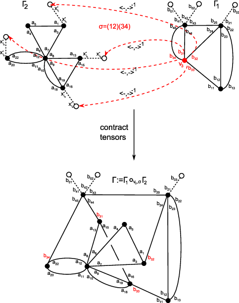
Refer to caption
Figure 6. Contracting tensors according to the pre-Lie structure on 𝔩n\mathfrak{l}^{n} corresponds to inserting one graph into another.

∎

This yields the following nongraphical description of the Connes-Kreimer Hopf algebra.

Corollary 3.14.

There is a natural isomorphism of Hopf algebras

𝒰^​(𝒫​𝔩+∞)→ℋ^+,x1⊗^⋯⊗^xk↦Φ−1(x1)⋆⋯⋆Φ−1(xk).\begin{array}[]{ccc}\widehat{\mathcal{U}}(\mathcal{P}\mathfrak{l}^{\infty}_{+})&\to&\widehat{\mathcal{H}}^{+},\\ x_{1}\hat{\otimes}\cdots\hat{\otimes}x_{k}&\mapsto&\Phi^{-1}(x_{1})\star\cdots\star\Phi^{-1}(x_{k}).\end{array}
Proof.

This follows from Theorem 3.13 and Theorem 2.18. ∎

References

  • [BP57] N. N. Bogoliubow, O. S. Parasiuk; Über die Multiplikation der Kausalfunktionen in der Quantentheorie der Felder. (German) Acta Math. 97 1957, 227-–266.
  • [Co84] J. C. Collins, Renormalization. An introduction to renormalization, the renormalization group, and the operator-product expansion. Cambridge Monographs on Mathematical Physics. Cambridge University Press, Cambridge, 1984.
  • [CK00] A. Connes, D. Kreimer; Renormalization in quantum field theory and the Riemann-Hilbert problem. I. The Hopf algebra structure of graphs and the main theorem. Comm. Math. Phys. 210 (2000), no. 1, 249–-273.
  • [CK02] A. Connes, D. Kreimer; Insertion and elimination: the doubly infinite Lie algebra of Feynman graphs. Ann. Henri Poincaré 3 (2002), no. 3, 411-–433.
  • [Cl11] K. Costello, Renormalization and effective field theory. Mathematical Surveys and Monographs 170. AMS, 2011.
  • [He66] K. Hepp, Proof of the Bogoliubov-Parasiuk theorem on renormalization. Comm. Math. Phys. 2 (1966), no. 1, 301–326.
  • [Ko93] M. Kontsevich, Formal noncommutative symplectic geometry. The Gelfand Mathematical Seminars, 1990-1992, pp. 173–187, Birkhäuser Boston, Boston, MA, 1993.
  • [Lo98] J. L. Loday, Cyclic homology. Second edition. Grundlehren der Mathematischen Wissenschaften, 301. Springer-Verlag, Berlin, 1998.
  • [MM65] J. W. Milnor, J. C. Moore; On the structure of Hopf algebras. Ann. of Math. (2) 81 1965 211–-264.
  • [Zi69] W. Zimmermann, Convergence of Bogoliubov’s method of renormalization in momentum space. Comm. Math. Phys. 15, 1969, 208-–234.