Inflationary perturbation theory is geometrical optics in phase space
Abstract
A pressing problem in comparing inflationary models with observation is the accurate calculation of correlation functions. One approach is to evolve them using ordinary differential equations (“transport equations”), analogous to the Schwinger–Dyson hierarchy of in–out quantum field theory. We extend this approach to the complete set of momentum space correlation functions. A formal solution can be obtained using raytracing techniques adapted from geometrical optics. We reformulate inflationary perturbation theory in this language, and show that raytracing reproduces the familiar “” Taylor expansion. Our method produces ordinary differential equations which allow the Taylor coefficients to be computed efficiently. We use raytracing methods to express the gauge transformation between field fluctuations and the curvature perturbation, , in geometrical terms. Using these results we give a compact expression for the nonlinear gauge-transform part of in terms of the principal curvatures of uniform energy-density hypersurfaces in field space.
I Introduction
Our current theories of the early universe are stochastic. They do not predict a definite state today: rather, their predictions are statistical. To compare these predictions with observation it must usually be supposed that we are in some sense typical. This brings two challenges. First, what is typical under some circumstances may be atypical under others. Therefore we must be precise about the type of observer of which we are a typical representative. This leads to the “measure problem,” about which we have nothing new to say. In this paper we are concerned with the second challenge: after fixing a class of observers, to estimate the observables typically measured by its members.
Inflation is the most common early-universe paradigm for which we would like to compute observables. In this context we usually take ourselves to be ordinary observers of the fluctuations produced on approach to a fixed vacuum. The challenge is to calculate the typical stochastic properties of these fluctuations.
The most important fluctuation generated by inflation is the primordial density perturbation, . Correlations in the temperature and polarization anisotropies of the microwave background are inherited from and provide a clean probe of its statistical character. Therefore, both present-day constraints [1] and the imminent arrival of high quality microwave-background data [2, *Ade:2011ah] make accurate estimates of its statistical properties a pressing issue. Meanwhile, large surveys of the cosmological density field will provide information about its properties on complementary, smaller scales [4]. To compare this abundance of data to models we require an efficient tool with which to estimate the -point functions .
Taking to be synthesized from the fluctuation of one or more light scalar fields during an inflationary era, several computational schemes exist which enable the -point functions to be studied. Many of these schemes employ some variant of the separate universe picture [5, *Lyth:1984gv, *Sasaki:1995aw, *Salopek:1990jq, *Sasaki:1998ug, *Wands:2000dp]. Taking to be the Hubble parameter, this asserts that—when smoothed on some physical scale, , much larger than the horizon scale, so that —the average evolution of each -sized patch can be computed using the background equations of motion and initial conditions taken from smoothed quantities local to the patch. Working from a Taylor expansion in the initial conditions for each patch, Lyth & Rodríguez showed how this assumption could be turned into a practical algorithm for calculating correlation functions [11]. This “ method” has become the most popular way to explore the predictions of specific models, both analytically and numerically, and has developed a large literature of its own. The principal difficulty arises when calculating the coefficients of the Taylor expansion, sometimes called the “ coefficients.” We shall discuss this difficulty in §IV.2.
Alternative approaches exist. Rigopoulos, Shellard & van Tent [12, *Rigopoulos:2005xx] evolved each correlation function using a Langevin equation. Yokoyama, Suyama & Tanaka [14, *Yokoyama:2007dw, *Yokoyama:2008by] decomposed each coefficient into components which could be computed using ordinary differential equations. Later, a systematic method to obtain ‘transport’ equations for the entire hierarchy of correlation functions (rather than simply the coefficients) was introduced [17, *Mulryne:2010rp]. A more longstanding approach uses the methods of traditional cosmological perturbation theory (“CPT”) to produce “transfer matrices” [19]. This has recently been revived by a number of authors [20, 21, 22, *Peterson:2010mv, *Peterson:2011yt, 25, 26]. Numerical approaches have been employed by Lehners & Renaux-Petel [27], Ringeval [28, *Martin:2006rs], and Huston & Malik [30, *Huston:2011vt].
The relationship of these different methods to each other has not always been clear. Nor is it always obvious how to relate the approximations employed by each technique. In this paper we study the connections between many of these approaches using the formalism of Elliston et al. [32]. This is a statistical interpretation of the separate universe picture. In what follows we briefly summarize the construction. (See also Ref. [17, *Mulryne:2010rp].)
The separate universe approximation as statistical mechanics.—Fix a large spacetime box of comoving side containing the region of interest. The scale should be much larger than the separate universe scale, requiring , but not superexponentially larger [33, *Lyth:2006gd, *Seery:2010kh]. After smoothing on the scale , the fields within the large box pick out an ensemble or cloud of points in the classical phase space. The condition that is not superexponentially large means that the typical diameter of the cloud will be roughly of order the quantum scatter . Because is still large, , it is convenient to describe the ensemble by an occupation probability on phase space.11 1 To be certain that we are estimating only the observables measured by a typical observer living within a single terminal vacuum, we should demand that has support only on points whose orbits eventually converge in some neighbourhood of that vacuum. This requires that all horizon volumes reheat almost surely in the same minimum. If some horizon volumes reheat in different minima then the resulting correlation functions are not measurable by a local observer who sees only a single vacuum. The correlation functions of on the scale are then determined by the classical statistical mechanics of this ensemble, which is encoded in the Boltzmann equation.
In familiar applications of statistical mechanics, the evolution of the ensemble may be complicated. Small-scale interactions scatter members of the cloud between orbits on phase space, represented by the collisional term in the Boltzmann equation. However, the separate universe assumption requires causality to suppress those interactions which would be required for scattering between orbits. Therefore the evolution is trivial. Each point in phase space is assigned an occupation probability by the initial conditions, which is conserved along its orbit. All that is required is a mapping of initial conditions to the final state, which is obtained by carrying the initial conditions along the phase space flow generated by the underlying theory. It follows that the Boltzmann equation can be integrated using the method of characteristics.
A similar conclusion applies to the correlation functions of interest, . These probe information about the distribution function over the cloud, giving a weighted average over many characteristics. Alternatively, if the cloud has only a small phase-space diameter, we can exchange information about the entire set of characteristics for the details of a single fiducial characteristic and a description of how nearby characteristics separate from it. In differential geometry this description is provided by the apparatus of Jacobi fields; see Fig. 1.
We shall see that the differing implementations of the separate universe approximation can be understood as alternative methods to compute these Jacobi fields.
In applications we are frequently interested in correlation functions associated with mixed scales, rather than a single scale . To do so we construct multiple ensembles associated with different smoothing scales. The separate universe approximation couples the evolution of all these ensembles in a specific way, which we describe in §III.
Outline.—In this paper we develop and refine the statistical-mechanical interpretation of the separate universe picture summarized above. Because the final distribution of occupation probabilities is an image generated by dragging along the phase space flow, it can be calculated in precisely the same way that geometrical optics enables us to calculate the image generated by a source of light rays. In §II we show that, at least within the slow-roll approximation, this parallel is exact; the scalar field equation can be interpreted as the eikonal equation for a light ray in a medium with varying refractive index—or equivalently as Huygens’ equation for a wavefront.
In §§II.3–II.4 we introduce the idea of Jacobi fields and explore their connection with the “adiabatic limit,” in which all isocurvature modes decay and the curvature perturbation becomes conserved. Such limits are important because an inflationary model is predictive on its own only if the flow enters such a region [36, 37, *Wands:1996kb, 39, 32]. Jacobi fields are familiar from the description of congruences of light rays in general relativity [40, 41]. In this case, as shown in Fig. 1, they describe fluctuations between the -sized patches which make up the ensemble. Their evolution enables the adiabatic and isocurvature modes to be tracked. In particular, decay of isocurvature modes means decay of the corresponding Jacobi fields, which occurs when the bundle of trajectories undergoes focusing.
In §III we use these ideas to develop evolution (“transport”) equations for each correlation function, and in §IV we show that the Jacobi fields can be used to formally integrate the system of transport equations. This gives a practical method to identify regions where the flow becomes adiabatic. The analysis can begin from either the separate universe principle or traditional cosmological perturbation theory. As a by-product, our formal solution demonstrates that the transport equations are equivalent to the Taylor expansion algorithm introduced by Lyth & Rodríguez.
In §IV.2 we use this solution to derive a closed set of differential equations for the Taylor coefficients, and in §IV.3 we explain how the transport equations can be manipulated to obtain evolution equations for the coefficients of each momentum “shape”. These shapes will be an important diagnostic tool when comparing inflationary models to observation [42, *Battefeld:2011ut]. Together with the transport hierarchy of §III, the equations of §§IV.2–IV.3 represent the principal results of this paper. Either set can be used to obtain the correlation functions of a given theory, and we discuss their comparative advantages.
In §IV.4 we give more a more general discussion of the relationship between the transport equations and other formulations of perturbation theory.
In §V we specialize to the slow-roll approximation and use ray-tracing methods to derive the gauge transformation between field fluctuations and the curvature perturbation, . As a result, we obtain the gauge transformation in terms of geometrical quantities—in particular, the extrinsic curvature of constant density hypersurfaces. We separate the gauge contribution to into a number of effects, corresponding to these geometrical quantities. For some models, we show that the largest of these can be attributed to a strong relative enhancement of the power in isocurvature fluctuations. We briefly discuss what conclusions can be drawn regarding the asymptotic magnitude of .
Finally, we provide a brief summary of our results in §VI.
II Geometrical optics in phase space
Throughout this paper, our discussion will apply to an inflationary phase which can be described by a collection of canonical scalar fields coupled to Einstein gravity. We initially use Greek labels , , …, to label the different species of fields. The action for this system is
| (1) |
where is an interaction potential depending only on the scalar fields, and indices , , …, run over space time dimensions. We take the background geometry to be flat Friedmann–Robertson–Walker with scale factor .
II.1 Slow-roll approximation: rays on field space
In this subsection we impose the slow-roll approximation. This requires where is the Hubble parameter. We introduce an -parameter for each species of light field,
| (2) |
in terms of which one can write . The slow-roll approximation therefore entails .
Huygens’ equation.—Combining (2) and the field equation for , and making use of the slow-roll approximation, we find
| (3) |
where measures the number of e-foldings of expansion experienced along the trajectory, and denotes a partial derivative with respect to . Eq. (3) constrains the canonical momenta to lie on a submanifold of the classical phase space coordinatized by the fields . This simplification is a consequence of the slow-roll approximation. In a theory with scalar fields, it implies that we may work with the simpler -dimensional field space instead of the full -dimensional phase space. This is convenient, although when we later abandon the slow-roll approximation we will have to return to phase space.
In what follows we often rewrite (3) in the form
| (4) |
and interpret the solution as an integral curve of the vector field , parametrized by . The scale is arbitrary. Since is a gradient, these integral curves correspond to pure potential flow.22 2 Since , it follows that is monotone decreasing along each integral curve. Therefore one may loosely think of as a Lyapunov function (or Morse function) for the flow.
The unit vector parallel to is
| (5) |
where we have defined
| (6) |
It follows that the arc length along an integral curve, labelled and measured using a flat Euclidean metric on field space, satisfies . Reparametrizing each curve in terms of , the flow equation (4) can be rewritten
| (7) |
where is Hamilton’s characteristic function. Eq. (7) is Huygens’ equation. Under the assumptions of geometrical optics, it describes the propagation of a light ray in a medium of spatially varying refractive index .
Snell’s law.—We conclude that the inflationary trajectories in field space are precisely the light rays of geometrical optics, for which Huygens’ equation can be thought of as a generalization of the Ibn Sahl or Snell–Descartes law. The wavefronts correspond to level sets of the characteristic function and are therefore equipotentials, or surfaces of constant energy density in field space. Each light ray is locally orthogonal to these surfaces, so the vector is locally the unit vector normal to a surface of constant energy density.
When slow-roll is a good approximation is small, , and increases to near the end of inflation.
II.2 Rays on phase space
In some circumstances the slow-roll approximation is not available. This may be the case during inflation if slow-roll is temporarily violated—perhaps during a turn in field space, to be studied in §V.2—or on approach to the end of inflation, where .
In such cases we must return to the full second-order field equation, which cannot be written in the form of Eq. (3). To obtain an analogue of geometrical optics one must pass to a Hamiltonian formalism. We define
| (8) |
This plays the role of Huygens’ equation for . In terms of , the scalar field equation becomes
| (9) |
We must also rewrite and in terms of , obtaining
| (10a) | ||||
| (10b) | ||||
Note that is purely a function of , whereas is a function of both and .
Eqs. (8)–(9) show that, beyond slow-roll, the precise analogy with Huygens’ equation is lost. Although these equations define a congruence of rays in phase space, it is not possible to find a characteristic function so that these rays are everywhere orthogonal to equipotentials of . Such a function would have to satisfy , and therefore for arbitrary . Unfortunately, there is no choice for which reproduces the right-hand side of Eq. (9).
The majority of our analysis requires only the first-order evolution equations (8)–(9), and at this level the formalism we develop will apply to evolution in phase space without imposing slow-roll. For that purpose it is convenient to combine and into a single phase-space coordinate. We continue to write this , with the understanding that now ranges over the dimensions of phase space. The velocity vector is likewise .
II.3 Jacobi fields and beam cross-sections
To proceed, we must carry the initial distribution of occupation probabilities along the flow, forming the “image” distribution of interest. In optical language, our task is to understand how images generated from a source of light rays are distorted by passage through a medium.
It was explained above that the typical spacing between arbitrarily selected members of the ensemble should be roughly of order the quantum scatter, . Because , this is small in comparison with the natural scale . Therefore the orbits traversed by the cloud trace out a narrowly-collimated spray or “bundle” of light rays in phase space. In canonical models of inflation, setting initial conditions near horizon-crossing will make the initial profile close to Gaussian [44]. Therefore the evolution of the ensemble is similar to the evolution of tightly-focused Gaussian laser beam propagating in an optical cavity.
Connecting vectors.—Cross-sections within the laser beam may be focused, sheared or rotated by refraction. These possibilities are familiar from the study of weak gravitational lensing.
To obtain a quantitative description we slice the laser beam open, generating a cross-section. The precise slicing is arbitrary. For applications to inflation we will often slice along surfaces of fixed energy density, or after a fixed number of e-folds. Distortions of the cross section can be studied if we know how an arbitrary basis is transported from slice to slice. In general relativity this would be Fermi-Walker transport [40].
Jacobi used this method to study geodesic deviation on Riemannian manifolds. For this reason an infinitesimal vector propagated along the beam is called a Jacobi field. Taking to be such a field and the flow vector to be sufficiently smooth, it will be transported by the equation
| (11) |
The quantity is the expansion tensor. It can be expanded in terms of a dilation , a traceless symmetric shear and an antisymmetric twist ,
| (12) |
where for flows on field space, or if we do not impose the slow-roll approximation and work on the full phase space. In either case is the Kronecker .
Optical scalars.—Dilation describes rigid, isotropic rescaling of by . It represents a global tendency of the light rays to focus or defocus. The shear is a symmetric square matrix and can therefore be diagonalized, yielding eigenvalues and corresponding eigenvectors representing the principal shear directions (here is a label taking values ; see §V.2). The shear describes a rescaling of the component of the connecting vector in the direction by a factor . Tracelessness of implies , so expansion in one direction must be accompanied by contraction in another. Therefore shear preserves cross-sectional area. Finally, the twist describes a rigid volume-preserving rotation of , representing a tendency of neighbouring trajectories to rotate around each other.
It is useful to define to satisfy
| (13) |
Imposing the slow-roll approximation and working on field space, the flow is orthogonal to equipotentials of Hamilton’s characteristic function. Therefore it is a pure potential flow, for which . On the full phase space this property is lost and the twist can be non-zero. In such cases it is helpful to define . Together, , and comprise the optical scalars introduced by Sachs and Penrose [45, *Penrose:1966].
van Vleck matrix.—Eq. (11) has a well-known formal solution in terms of an ordered exponential [47]. This method was used Rigopoulos, Shellard & van Tent [48, *Rigopoulos:2005us], and later by Yokoyama et al. [14]. It yields an explicit (but formal) expression for transport of any Jacobi field along the beam,
| (14) |
where is the Jacobi field on some initial slice . Eq. (14) describes the evolution of this Jacobi field at any later time . The matrix satisfies
| (15) |
where the path-ordering operator rewrites its argument with early times on the right-hand side, and later times on the left. We will occasionally refer to as the propagator matrix. It is closely related to a Wilson line.
Index convention.—Eq. (15) can be simplified with the aid of an index convention. Up to this point we have been labelling field-space indices using Greek symbols , etc. To avoid writing the time of evaluation explicitly, we adopt the convention that Greek indices denote evaluation at the late time of interest, . Latin indices , , etc., denote evaluation at the early time . Therefore can be written as a mixed index object, .
Eq. (14) immediately implies
| (16) |
and endows this derivative with a geometric interpretation. It plays an important role in the Lyth–Rodríguez implementation of the separate universe approximation [11], where it appears due to a Taylor expansion in the initial conditions local to each -sized patch. In this formulation, one often projects on to equipotential surfaces in field space. We define to obtain
| (17) |
The notation ‘’ indicates that can be thought of as the variation of a field defined on a fixed comoving spacetime hypersurface [50, 51, *Seery:2006js]. It follows from geometrical aguments that , where is the unit normal to phase-space slices of constant potential energy, defined in (5). The tensor is the induced metric (or “first fundamental form”) on these surfaces. Eq. (17) shows that choice of gauge is associated with projection onto an appropriate hypersurface in phase space. Moreover, Eqs. (16)–(17) show that partial derivatives with respect to are associated with propagation of Jacobi fields along the bundle.
Caustics.—The matrix appears whenever it is necessary to track the distortion of a line element along a flow, and has applications in fluid dynamics, general relativity and elsewhere [40, 53]. DeWitt–Morette observed that, considered as a matrix of Jacobi fields, Eq. (16) was related to the inverse of the van Vleck matrix, introduced in the construction of semiclassical (“WKB”) approximations to the path integral [54, *DeWittMorette:1984du, *DeWittMorette:1984dw].33 3 In DeWitt–Morette [54] the proof is ascribed to B.S. DeWitt. DeWitt–Morette noted that the relation between Jacobi fields and variation of a general solution of the field equations with respect to its constants of integration had been known to Jacobi (ultimately leading to his development of what is now Hamilton–Jacobi theory), and suggested that this technique could be used to simplify the long calculations which arise when solving Jacobi’s equation. Applied to inflationary correlation functions, the history has been reversed: the variational formulae came first, in the form of the Lyth–Rodríguez algorithm. This often leads to simple analytic results, as DeWitt–Morette foresaw. But, as we explain in §IV.2, this method is unsuited to numerical implementation, because of the small numerical tolerances required to reliably determine variation with respect to the initial conditions. It is preferable to solve an ordinary differential equation, such as Jacobi’s equation (11) or (25). We define
| (18) |
The van Vleck matrix is , and has a well-known interpretation in geometrical optics as a measure of focusing or defocusing: in particular, at a caustic, where light rays converge. Since is nonzero for , a singularity in the van Vleck determinant implies a singularity in . Applying (12), we conclude
| (19) |
Therefore at a caustic. This happens after finitely many e-folds only if during the flow. Otherwise, is decreasing in regions where is negative, with large negative implying strong focusing. Large positive implies strong defocusing. More generally the propagator matrix can be rewritten in terms of , giving
| (20) |
The ordered exponential has determinant unity and therefore does not change the cross-sectional area of the bundle.
II.4 Adiabatic limit
Caustics have an important interpretation in the flows describing an inflationary model. If the bundle of trajectories has finite cross section, then the ensemble contains members which are evolving along multiple phase space trajectories. These are the eponymous “separate universes” with their individual initial conditions.
Under these circumstances one or more isocurvature modes exist. These are connecting vectors which relate the different within the bundle which all lie on a surface of fixed energy density, say . Their number is determined by the rank of . In the special case where the bundle cross-section decays to a point, there is a unique intersection between the bundle and . Therefore has rank zero and all isocurvature modes disappear. In this limit, each member of the ensemble traverses the same orbit, differing from the others only by its relative position, which corresponds to the adiabatic mode, . It follows that, when the cross-section collapses to a point, the fluctuations become purely adiabatic. Elliston et al. [32] described this as an ‘adiabatic limit’. After this limit has been reached is conserved [57, 58].
Flows which reach an adiabatic limit during inflation are no more or less likely—or natural—from the viewpoint of fundamental physics. But flows reaching an adiabatic limit are more predictive, because a perturbation in the purely adiabatic mode remains adiabatic long after inflation ends [59, *Weinberg:2008si], even during epochs for which we are ignorant of the relevant physics. Contrariwise, if any isocurvature modes remain then members of the ensemble may rearrange their relative positions until these modes decay. This possibility was emphasized by Meyers & Sivanandam [61, *Meyers:2011mm]; see also Ref. [32]. If the flow does not reach an adiabatic limit during inflation then the model is not predictive until we supply a prescription for the post-inflationary era, and observational predictions can depend on this choice.
Trivial, adiabatic and nonadiabatic caustics.—The outcome of this discussion is that approach to an adiabatic limit can be associated with convergence to a caustic. An early discussion of this principle, phrased almost precisely in these terms, was given by Wands & García-Bellido [38]. We conclude that is a necessary condition for an adiabatic limit to occur, but as we now explain it is not sufficient.44 4 One may have some reservations about this conclusion, because it seems to violate the Liouville theorem which guarantees conservation of phase-space volume. However, it should be remembered that the canonical phase space coordinate to which Liouville’s theorem applies are not the field-space position and momenta which we are using. In particular, the canonical momenta will typically include powers of the scale factor . A caustic can be classified by the number of dimensions lost by the flow, or equivalently the number of null eigenvalues of the propagator at the caustic. An adiabatic limit is the special case where retains a single non-null eigenvalue, but has no non-null eigenvalues. We describe caustics which satisfy this condition as adiabatic.
Eq. (20) shows that, were the integrated shear and twist to remain bounded while , then . In this case no perturbations would survive, and we describe the caustic as trivial. An example is the case where is pure dilation. But barring an accurate cancellation of this kind, at least some component of will typically scale proportionally to on approach to the caustic.55 5 In principle could contain off-diagonal terms which grow faster than the diagonal terms, and therefore . In this case there could be a subspace of growing perturbations. If the growth is exponential this usually signals an instability, and the formalism we are describing becomes invalid.
Shear opposes focusing.—If the perturbations are not to vanish completely, then some anisotropic effect of shear and twist must oppose the isotropic contraction due to .
First suppose the twist is negligible. We assume that the eigenvectors of stabilize in the vicinity of the caustic. If the shear has some number of positive eigenvalues for which has a finite, nonzero limit, then perturbations may survive in the subspace spanned by their corresponding eigenvalues. Tracelessless of implies that at least one eigenvalue must be negative, and perturbations in the subspace spanned by the corresponding eigenvectors will disappear. Hence, at least one dimension will be lost by the flow. In practice it is often simpler to work directly with the eigenvalues of the expansion tensor .
If more than one eigenvalue of is positive, then perturbations may survive in a two- or higher dimensional subspace. In this case the caustic does not describe approach to an adiabatic limit, and we call it nonadiabatic. To obtain predictions for observable quantities the evolution must be continued. In practice this would require introduction of a reduced phase space describing only the surviving perturbations. The flow can then be followed in this reduced phase space until a further focusing event occurs. This may itself be an adiabatic limit, or might simply describe further reduction in the phase space. One should continue in this way until an adiabatic limit is finally achieved. An example of this behaviour could occur soon after the onset of slow-roll inflation. In the early stages, independent fluctuations in the field velocities survive. But when slow-roll is a good approximation these will be exponentially suppressed, making become very small. One should therefore replace the full description by a reduced phase space which includes only field perturbations. In doing so one arrives at the field-space description of slow-roll inflation given in §II.1.
Twist opposes focusing.—In slow-roll inflation, which we discuss in §II.5 below, a diverging shear is the only mechanism by which perturbations can survive on approach to a caustic. Where the twist is non-zero, which occurs when we do not impose the slow-roll approximation, more possibilities exist. Ultimately these must be addressed, to describe approach to an adiabatic limit when slow-roll is no longer a good approximation, but we defer this discussion for future work.
II.5 Focusing in the slow-roll approximation
In this subsection we give a more detailed discussion of the approach to a caustic during an era of slow-roll inflation.
Raychaudhuri equations.—Parametrizing each trajectory by e-folding number , Eq. (4) constitutes an autonomous dynamical system. Therefore a derivative along the flow can be written . In the absence of a nontrivial field-space metric all derivatives commute, and therefore . Contracting with and rearranging terms, one finds
| (21) |
where is the acceleration vector, defined by . For a potential flow, this can be simplified; comparison with Eq. (4) shows that
| (22) |
where, as above, is the local refractive index.
The evolution equations for the dilation and shear can be written
| (23a) | ||||
| (23b) | ||||
These are commonly known as the Raychaudhuri equations. An equation for the evolution of the twist could be found in the same way, but is not needed in the slow-roll approximation.
We have defined to be the Hessian of ,
| (24) |
and is its trace. Because the Hessian measures the local curvature of a function, one can regard as a measure of the curvature of surfaces of constant refractive index in field space.
Jacobi equation.—Eq. (11) shows that Jacobi fields oriented along eigenvectors of with positive eigenvalues grow, whereas those oriented along eigenvectors with negative eigenvalues decay.
We can find an alternative description in terms of the refractive index . Taking a derivative of (11) along the flow and using the Raychaudhuri equations to eliminate derivatives of the dilation and shear yields the Jacobi equation,66 6 When using Jacobi fields to study geodesic deviation on a Riemannian manifold, this equation takes the form , where is a component of the Riemann curvature projected along the tangent to the geodesic.
| (25) |
It follows that the behaviour of the Jacobi fields is determined by the curvature of , considered as a function in field space. (Note this is related to, but not the same as, the curvature of surfaces of constant .) Qualitatively, Jacobi fields oriented along eigenvectors of with negative eigenvalues—directions of negative curvature—will have quasi-trigonometric solutions. These will pass through zero, corresponding to the collapse of some Jacobi fields to zero length. Fields oriented along eigenvectors with positive eigenvalues will have exponential solutions. Unless the initial conditions are precisely adjusted, these will typically grow.
Focusing theorem.—By adapting the geodesic focusing theorem of general relativity [40] we can determine the circumstances under which focusing will occur after finitely many e-folds. Pick a point on the flow where the expansion is negative, with value . Inspection of (23a) shows that, if , then within e-folds, where is the dimension of field space. Any point where is a caustic, because on arrival at this point .
Since Morse’s lemma implies that is negative in a neighbourhood of any local maximum of the refractive index, , one might hope to associate such local maxima with terminal points for inflation at which an adiabatic limit would be nearly achieved.
However, the conditions of the focusing theorem are not satisfied for typical potentials. More usually the slow-roll approximation forces all fields to settle into a terminal vacuum increasingly slowly, requiring an infinite number of e-folds to reach . Moreover, in practical examples the slow-roll approximation will break down and inflation will terminate long before the caustic is reached. Therefore we should not expect to achieve precisely during inflation. Nevertheless, a model may be sufficiently predictive if the flow spends enough e-folds in a region of large negative that is exponentially suppressed before inflation ends.
In simple potentials it is often clear when ceases to evolve. But for more complicated potentials the situation may not be so clear. Within the slow-roll approximation, this discussion shows that can be taken as a clear indication that isocurvature modes are still present. Their future decay is likely to influence and the outcome of any calculation which terminates with should not be considered a prediction for observable quantities. Conversely, is an indication that some decay of isocurvature modes has taken place. The precise nature of the decay must be deduced from the behaviour of the shear and twist. If perturbations survive only in a one-dimensional subspace than we can infer that the isocurvature modes have decayed to the point that will be approximately conserved.
Example: quadratic Nflation.—We illustrate these ideas using the quadratic approximation to Nflation [63, 64, *Kim:2010ud, *Kim:2011jea]. The potential is
| (26) |
This model is of interest in its own right, but also describes the approach to a generic stable minimum after suitable choice of field space coordinates. We suppose that there is at least a modest hierarchy among the masses, and order these so that if . The most massive field will settle into its minimum first, followed by the next most massive field. Therefore approach to the final minimum will be described by a trajectory on which only is dynamical, with all other approximately zero. We describe this as the “inflow” trajectory.
On the inflow trajectory, the dilation satisfies
| (27) |
The minimum is a caustic, but as discussed above it cannot be reached after finitely many e-folds (within the slow-roll approximation). The expansion tensor satisfies
| (28) |
This has one positive eigenvalue and the rest negative, so we expect it will correspond to an adiabatic limit.
The component of diverges near the caustic. This does not signal an instability, but only that grows at precisely the required rate to give constant .
Ordered exponentials such as (15) satisfy a composition property, allowing the integral over the inflationary trajectory to be broken in two. (See Fig. 2.) The first component is an integral from the initial point until the onset of the inflow trajectory. We take this to occur at , and choose so that (28) is a good approximation there. The propagator at this point is . It is a complicated weighted average over the trajectory, and cannot usually be calculated analytically. The second component is an integral over the inflow trajectory, which we denote . Therefore . The inflow part can be computed from (28),
| (29) |
Except perhaps for special choices of initial conditions, Eq. (29) gives rank at the caustic. Therefore this is an example of an adiabatic caustic.
In more general circumstances, it may be necessary to diagonalize before integrating over the inflow trajectory. This is reminiscent of the introduction of scaling operators in a renormalization-group framework. Indeed, the entire analysis, and the emergence of rational but non-integer power-law scaling near the caustic, parallels a renormalization group analysis in the neighbourhood of a fixed point [67]; compare also Eq. (79) of Vernizzi & Wands [50].
Focusing in double quadratic model.—Away from the inflow trajectory it is usually necessary to proceed numerically. In Fig. 3 we show the evolution of the focusing parameters in the well-studied model of double quadratic inflation [68, 36, 37, 39, 50, 69, 48, *Rigopoulos:2005us]. The potential is . We choose the mass ratio and set initial conditions and .
Initially the evolution is mostly in the direction. When reaches the vicinity of its minimum there is a turn in field-space, which generates a spike in . After the turn, the inflow trajectory is reached along the direction.
This evolution is reflected in the evolution of the bundle. Initially and the cross-section slowly dilates. It reaches a maximum at roughly three times the original cross-sectional area. After the turn, rapidly drops to a negative value, and thereafter diverges exponentially to . Therefore the bundle-cross section very rapidly diminishes to almost zero cross-sectional area. This corresponds to an approximate caustic, and leads to an adiabatic limit.
Eventually the divergence in would be cut off by a breakdown of the slow-roll approximation, but for typical parameter choices will already be exponentially small at this point.


Example: axion-quadratic model.—Elliston et al. [32] introduced an approximation to the hilltop region of axion N-flation [65, *Kim:2011jea]. The Hubble rate is dominantly supported by many axions in the quadratic region of their potential, and can be approximated by a single field. A few axions remain in the vicinity of the hilltop, where their contribution to is negligible but their contribution to the three- and higher -point functions in the adiabatic limit is large.
The potential is . We set and choose . In Fig. 4 we show the evolution for initial conditions and .
The evolution is similar to the double quadratic model. Initially is positive and the cross-sectional area grows. At its peak, it is more than 200 times the original cross-section. Eventually approaches its minimum and the Hubble friction decreases to the point that can evolve. It rolls away from the hilltop, eventually ending inflation. During this phase switches sign, ultimately diverging exponentially to . Therefore we approach an adiabatic limit. However, Fig. shows that the rate of approach is quite slow. The cross-section decays softly, and by the end of inflation . Therefore an approximate adiabatic limit is reached and we can expect the observables to be roughly conserved through the post-inflationary evolution.


III Transport equations
We now apply these ideas to obtain evolution (or “transport”) equations for the correlation functions in a fixed, comoving spacetime volume. In this section our analysis will be general, and can be applied to any perturbations whose evolution equations can be expressed in the form of Eq. (31). If necessary this can be achieved as described in §II by passing to a Hamiltonian framework. It follows that the transport of correlation functions is most naturally expressed in phase space.
Connecting vectors.—Consider the set-up described in §I, in which a comoving spacetime region of size is smoothed into separate universes of size . Pick any one of these -sized regions, which we take to be at spatial position . The separate universe approximation asserts that the evolution of the smoothed fields in this region is given by the flow equation (4). We denote the difference between these values and those in some other region, located at position , by . This is a connecting vector in the sense of Eq. (11). Taylor expanding , the corresponding deviation equation is
| (30) |
We assume and have subtracted a zero-mode to preserve this throughout the motion.77 7 In the language of Feynman diagrams, this would correspond to removing contributions arising from disconnected pieces. This procedure is routine in applications of the separate universe principle. The tensor was defined in (11), and . We describe them, together with higher-index counterparts obtained by further differentiation, as -tensors. They inherit a dependence on through evaluation at . After transformation to Fourier space, the subtractions in Eq. (30) correspond to discarding disconnected correlation functions. Therefore statistical properties of the ensemble do not depend on our choice of fiducial point.
If is not superexponentially large, we can typically expect to be small and slowly varying. In Fourier space, this implies that is constructed from only a few soft, infrared modes which we label . The remaining modes have been integrated out in the smoothing process used to obtain this effective, separate-universe description. Working explicitly in terms of these modes, Eq. (30) yields a connecting vector and deviation equation for each combination of species and -mode88 8 In Eq. (31) we are keeping nonlinear terms in the evolution equation. We use the term “Jacobi field” to refer to infinitesimal connecting vectors, for which only the linear term need be kept.
| (31) |
Eq. (31) has been written in an abbreviated “de Witt” notation, in which the primed, compound index carries both an unprimed species (or “flavour”) label and a momentum . Contraction over primed indices implies summation over the flavour label and integration over the momentum label with measure . The 2- and 3-index -tensors appearing here satisfy
| (32a) | ||||
| (32b) | ||||
Eq. (30) was given by Yokoyama et al. [14, *Yokoyama:2007dw] in real space, and used to obtain evolution equations for the momentum-independent Lyth–Rodríguez Taylor coefficients. We explore the relationship between our approaches in Appendix A. However, Yokoyama et al. did not interpret as the expansion tensor of the flow or give the -space equations (31) and (32a)–(32b). As we will see, this -dependent information is necessary to obtain transport equations for the full set of coupled -space correlation functions.
One can arrive at the same conclusions using cosmological perturbation theory. Taking the background value of to be the average field over the -sized box, the perturbations within the box are . One should now interpret as a coordinate relative to the box. Restricting attention to the infrared modes in , for which is negligible, we recover Eqs. (31) and (32a)–(32b).
Correlation functions.—The full set of connecting vectors contains all information required to determine evolution of the bundle, and therefore the evolution of all statistical quantities. In Eq. (31) this data is carried by the -tensors. The transport equations for correlation functions are simply a reorganization of this information. Therefore they must also be expressible purely in terms of -tensors. Since (31) shows that these tensors can be obtained by the separate universe argument or traditional perturbation theory, it follows that they will make equivalent predictions.
There are multiple ways to organize the -tensors to produce evolution equations. In Ref. [17, *Mulryne:2010rp], transport equations were obtained after postulating a conservation equation for a probability density ,
| (33) |
Evolution equations for the moments of were extracted using both a Gauss–Hermite expansion, and generating functions. Here we describe a third, simpler method. Provided the perturbations can be treated classically, we expect for any quantity .99 9 This equation both implies and is implied by conservation of probability, Eq. (33)
Two-point function.—We write the two-point function as . Eq. (31) implies
| (34) |
where is the matrix anticommutator of and , and [ 3 p.f.] denotes terms including three-point functions or above which have been omitted. In general, the transport equations will couple correlation functions of all orders. They can be thought of as a limiting case of a Schwinger–Dyson hierarchy, applied to expectation values rather than the in–out amplitudes of scattering theory. Calzetta & Hu argued that the result could be interpreted as a Boltzmann hierarchy [70, 71].
As in any effective theory, the transport equations will be useful only if a reason can be found to systematically neglect an infinite number of terms. Applied to inflation, the statistical properties of the ensemble are nearly Gaussian: in the simplest models, an -point function will typically be of order , where is the smallest even integer at least as large as [72]. This is suppressed compared to the natural scale by . However, this is not necessary; all that is required (or suggested by observation) for (34) to be valid is that the three- and higher -point functions are substantially smaller than the two-point function.
Eq. (34) was given in Ref. [17, *Mulryne:2010rp] for an arbitrary -field model, but with interpreted as the real-space correlation function. The single-field case is discussed by Gardiner [73]. With the -tensors given in (32a)–(32b), Eq. (34) applies for the full -dependent correlation function.
Three-point function.—We write the three-point function as . Keeping contributions of order and , we conclude
| (35) |
In simple models, the scaling estimate makes both terms the same order of magnitude. For (35) to be valid requires the 4-point function to be substantially smaller, which is also supported by observation [74, *Fergusson:2010gn].
IV Evolution of correlation functions
IV.1 Solution of the transport hierarchy by raytracing
The transport equations (34) and (35) can be solved using the machinery developed in §II. The key ingredients are the phase-space flows which describe evolution of individual “separate universes,” and the Jacobi fields which connect them. The solution is formal and depends only on the structure described in §III. Therefore there is no requirement to impose the slow-roll approximation, and when written over the full phase-space our equations apply quite generally. When truncated to field-space they reproduce the slow-roll evolution.
Two-point function.—We write the two-point function in the form
| (36) |
where is to be determined. This notation has been chosen because will turn out to be the propagator matrix (15) for the primed indices. Indeed, (36) is a solution of the transport equation (34) if
| (37a) | ||||
| (37b) | ||||
In writing (37b) we have assumed approximate Gaussianity, so that contributions from higher-order correlation functions are suppressed by at least a power of compared to the terms which have been retained. Keeping these terms would yield the “loop corrections” of the Lyth–Rodríguez formalism [33, 76, 77, *Seery:2007wf, 35]. To the order we are working, should be identified as a constant: it is the value of the two-point function evaluated at , where is the initial time which appears in the propagator (15). We write this constant value .
The primed propagator satisfies
| (38) |
where is the flavour propagator (15). Therefore, written more explicitly, Eq. (36) becomes
| (39) |
where our usual convention—that Latin indices denote evaluation of the correlation function at some initial time —continues to apply. For the two point function, practical calculations usually simplify if this is taken to be the horizon-crossing time associated with scale . We have indicated this by attaching a subscript ‘’ to the correlation function. With this understanding, and recollecting the identification (16), Eq. (39) is the familiar “” result [5, 7, 11].
Three-point function.—Similar methods can be used to solve for the three- and four-point functions. We write . As for the two-point function, the propagator matrices absorb contributions from the -tensors. In the case of there were no other terms, making the “kernel” time independent. Here, the presence of terms involving 3-tensors provides a source for . We find1010 10 We are allowing to be a function of , which means our index convention must be interpreted more abstractly. The expressions for -matrices to which Eq. (40) leads, such as Eqs. (49a)–(49b), can be interpreted in the original sense.
| (40) |
where, as above, is the initial value of the two-point function introduced in (36). The estimate for the truncation error, beginning with contributions from the four-point function, again assumes that the correlation functions order themselves in even powers of . We define the matrix to be the left-inverse of the propagator, . Inspection of (38) shows that it can be written
| (41) |
where is the conventional matrix inverse of the flavour propagator, Eq. (15). In what follows it is useful to define a projected 3-tensor, , by
| (42) |
Combining (38) and (41), it follows that the explicit - and flavour-dependence can be written
| (43) |
where the tensor is the obvious flavour projection of , so that .
With these definitions, Eq. (40) can be solved by quadrature. Up to loop corrections, we find
| (44) |
where should be regarded as the value of the three-point function at . The complete solution can be written (again up to loop corrections)
| (45) |
where the cyclic permutations exchange .
One can regard Eqs. (37a)–(37b) and (44) as analogous to the “line of sight” integral which is used to obtain a formal solution to the Boltzmann equation in calculations of the cosmic microwave background anisotropies.
The quantity is defined by
| (46) |
Observe that Eq. (46) is symmetric in the indices and . With our choices for the - and flavour-dependence of its constituent quantities, it can be written
| (47) |
where is the flavour-only object obtained by exchanging primed for unprimed indices in (46). Comparing with (15), it follows that (up to matrix ordering ambiguities) is the derivative of the propagator,
| (48) |
Eq. (45) can now be recognized as the Lyth–Rodríguez formula for the three-point function [11].
IV.2 Flow equations for “” coefficients
We conclude that the transport equations (34) and (35) are equivalent to the Taylor expansion algorithm of Lyth & Rodríguez for the three-point function. Also, because the -tensors could equally well be derived using the methods of cosmological perturbation theory, all these methods will give answers which agree. Within this narrow reading, our analysis can be interpreted as a demonstration that these methods are interchangeable. Therefore we believe that statements to the effect that any particular method currently in use has an intrinsic drawback when compared with another, as a matter of principle, are wrong.
Nevertheless it is true that some approaches have advantages in practice, although no one approach outperforms the others in all applications. For example, as explained in §I, in some models the Taylor expansion algorithm leads to very simple analytic formulae. This property has encouraged a large literature studying models to which the method can be applied.
In this broader context our analysis is not simply a reformulation of existing results. First, as a byproduct of the raytracing method we have obtained explicit (but formal) expressions for the Lyth–Rodríguez Taylor coefficients,
| (49a) | ||||
| (49b) | ||||
Analytically, the Taylor expansion method is useful only when a solution to (49a) can be found in closed form. This has been achieved only for a limited class of potentials obeying some form of separability criteria; a summary appears in Ref. [32] together with references to the original literature. Eq. (49a) clarifies the difficulty encountered in obtaining analytic formulae as the difficulty of computing closed-form expressions for a path-ordered exponential. A sophisticated theory is available [79] but explicit expressions can usually be obtained only in special cases, or where the expansion tensor commutes with itself at different times. It is possible that Eq. (49a) could be used to extend analytic progress beyond the separable cases, but we have not investigated this possibility in detail.
Eqs. (49a)–(49b) were given, in slightly different notation, by Yokoyama et al. [14, *Yokoyama:2007dw]. Because of its close relation to the present discussion we review and extend the Yokoyama et al. approach in Appendix A.
Second, a naïve numerical implementation of the Taylor expansion formula is unfavourable. Beginning with fractionally displaced initial conditions one must evolve the equations of motion over many e-folds, during which numerical noise is accumulating. Taking differences between these evolved solutions requires high-accuracy integration in order that the small displacement in initial conditions is not swamped by noise. The explicit solutions (49a)–(49b) allow this naïve approach to be replaced by a simple system of ordinary differential equations for and . The equation is the Jacobi equation (37a), after dropping primes on indices. The initial condition is . The equation can be obtained by differentiation of (49b). It is
| (50) |
with initial condition .
IV.3 Transport of “shape” amplitudes
The results of §IV.1 apply for arbitrary initial conditions , for the two- and three-point functions. But for application to inflation, we will usually wish to apply them to the correlation functions produced in a specific model. In this case the fields will be a collection of light scalars for which and can be computed using the in–in formulation of quantum field theory [44]. These yield very specific -dependences whose amplitudes we wish to track.
In this section, our analysis remains general and continues to apply to the full phase space.
Two-point function.—The two-point function is straightforward. For a nearly scale-invariant spectrum we have
| (51) |
where and the flavour matrix should be nearly independent of . Transport of can be accomplished using (39), or simply by solving the transport equation (34) with an appropriate initial condition after dropping primes on indices. That gives
| (52) |
where is the initial value of . The mild -dependence of (52) can also be obtained using transport techniques [80].
Three-point function.—Here, more possibilities exist. It is known that the terms in (45) dominate whenever the bispectrum is large enough to be observed [81, 50]. Eq. (45) shows that these contributions add incoherently to the contribution from , so they can be studied separately. Using (51) and overall symmetry of the correlation function under exchange of indices, we can write
| (53) |
where the notation “” indicates that the three-point contribution contains this contribution among others. The amplitudes are symmetric under exchange of and , but not otherwise. Using Eqs. (32a), (32b), (35) and (51), we find the transport equation
| (54) |
If desired, we can apply the same method of formal solution described in §IV.1. This yields
| (55) |
In combination with (53) this reproduces our earlier formula (45), neglecting the initial contribution .
IV.4 Connections between the transport and other approaches
Up to this point we have shown that the Jacobi fields which connect “separate universe” trajectories in phase space can be used to solve the transport equations for the full set of -space correlation functions. But as we have explained, the transport hierarchy is just one of many techniques for handling correlation functions. We now pause to examine the connections between these approaches.
formalism.—In the Lyth–Rodríguez approach, or “ formalism”, one makes a Taylor expansion of the field values on a final hypersurface in terms of field values on some initial hypersurface. Following the discussion surrounding Eq. (30), and with the same meaning for the vectors and , this can be written
| (56) |
Note that, despite appearances, we are making no assumption that the evolution of is close to an attractor. Therefore there is no requirement to invoke the slow-roll approximation. It is true that the existence of an attractor would make the canonical momenta purely a function of the fields, yielding an equation with the appearance of Eq. (56). But as we have explained, by working in a first-order Hamiltonian formalism we can obtain expressions such as (56) without this limitation. Therefore we allow the to include perturbations of the canonical momenta if necessary, in which case the indices , , etc. range over the dimensions of phase space. Where slow-roll is a good approximation we can revert to a simpler formulation based on field space.
We have already remarked that the -tensors are the derivatives (16) and (48). In Eq. (56) the are all defined on spatially flat hypersurfaces. More commonly, an analogous expansion is made for the total e-folding number , measured from a flat slice to a final comoving slice; we give an explicit relation in §V. The choice of slicing simply corresponds to the gauge in which we wish to work [18].
For (56) to be useful, some means must be found to compute and .
Flow equations.—As a by-product of the raytracing solution, or “line of sight” integral, we obtained the evolution equations (37a) and (50). These allow the -tensors to be computed easily. However, the same equations can be obtained directly from the separate universe formula, Eq. (56). Substituting (56) into both the right- and left-hand sides of (30) and separating the resulting expansion order-by-order, we immediately arrive at Eqs. (37a) and (50). This still does not require the slow-roll approximation.
Transfer matrices.—We have observed that Eq. (30) arises in the limit of cosmological perturbation theory (“CPT”). Within that framework, at least in the first-order theory, it is common to introduce “transfer matrices” which relate field perturbations at different times [19]. Typically these are chosen to be the adiabatic and isocurvature directions, but in principle any basis can be used.
Restricting to first-order, the transfer matrix is determined precisely by the leading term of (56), or a gauge transformation of it. It follows that Eq. (56) represents the extension of the transfer matrix to second-order (and beyond), and Eqs. (37a) and (50) give the evolution of the transfer tensors , . Therefore the transfer-matrix formalism is precisely equivalent to the separate universe picture and traditional cosmological perturbation theory. Note that if the perturbations are projected onto adiabatic and isocurvature modes this requires use of the correct tensors at each time step.
CPT implies transport equations.—Finally, we show that cosmological perturbation theory implies the transport hierarchy with which we began. We write
| (57) |
which, neglecting “loops,” follows from (56) and therefore either CPT or a transfer-matrix approach. Differentiating both sides with respect to time, recalling that is time-independent, and make use of (37a) we find
| (58) |
This gives the transport equation for , Eq. (34). A similar procedure leads to the transport equation for , Eq. (34). It follows that each of these approaches implies and is implied by the others.
V Gauge transformations
To this point, the formalism we have developed enables the correlation functions of fluctuations in the fields and their momenta, and , to be evolved along the bundle of trajectories picked out by an ensemble of smoothed regions. However, by themselves these fluctuations are not observable. Only specific combinations are observable, of which the most important is the primordial curvature fluctuation . Therefore to proceed we require expressions for the gauge transformation between the , and .
In this section we impose the slow-roll approximation throughout, enabling us to work on field space and make use of the hypersurface-orthogonal property of the flow. We intend to return to the general case in a future publication.
V.1 Explicit transformations
In the slow-roll approximation there is no need to track the momentum fluctuations , which are purely determined by the field fluctuations . Therefore can be written purely in terms of the field fluctuations.
On superhorizon scales, the appropriate gauge transformation can be written as a Taylor expansion,
| (59) |
where all fields are evaluated at the same spatial position and a constant has been subtracted to set . The Taylor coefficients and have been given by various authors [82, 17]. Working in field space, we give a purely geometrical derivation. This argument relies on the property that the flow is orthogonal to surfaces of constant density in field space, and therefore will not generalize directly to the full phase space.
Linear term.—Consider Fig. . We wish to compute the coefficient at a field-space point , which can be taken to lie on a hypersurface of fixed energy density . We denote this hypersurface . According to the separate universe approximation, can be computed from the number of e-folds required to flow back to after making a generic (“off-shell”) displacement from . Anticipating the discussion of second-order contributions, we denote this displacement and write .
The number of e-folds required to return to must be computed along the inflationary trajectory which passes through . In Fig. , this trajectory intersects at . The tangent to the trajectory at is the normal vector . Therefore the (“on-shell”) field-space displacement along this trajectory, to first order in , is . The symbol ‘’ denotes equality up to higher-order terms in which have been omitted, and we have adopted a convention in which quantities evaluated at —such as the unit vector —are written without an argument. Combining Eqs. (3) and (5), we conclude
| (60) |
and therefore
| (61) |
where we have reintroduced the refractive index defined in §II.1. Eq. (61) is the term in (59).
Quadratic term.—The quadratic Taylor coefficient can be obtained from the variation in under a second generic displacement . Under this displacement the origin is shifted to . Because the energy density at will typically differ from , it lies on a displaced hypersurface . However, the definition of is unchanged and must still be measured to the intersection with at . We should compute the flow along the trajectory passing through . The path is a discrete approximation to an integral along this flow. The calculation should be carried to linear order in and independently.
In Fig. , the on-shell flow from back to is . Repeating the analysis above, we find
| (62) |
where . (It is only necessary to work to first order in , since (62) is proportional to .) The on-shell flow from back to is
| (63) |
We have defined to be the displacement to ,
| (64) |
and . The symmetric tensor is the extrinsic curvature of , or “second fundamental form,” and is defined by [40]. It is related to the dilation and shear of the expansion tensor via
| (65) |
where is the projection of the shear onto the isocurvature subspace, . The first term in (63) is a linear, trigonometric approximation. The second is a correction for the curvature of . A similar construction could be used to obtain the Taylor coefficients at any desired order.
After computing all appropriate variations, we find
| (66) |
where is the natural generalization of the single-field -parameter. It measures the variation of along the adiabatic direction. To yield sufficient e-foldings, it must typically be small while observable scales are leaving the horizon. Defining to be a derivative along , it can be written
| (67) |
In addition, is a derivative in the plane tangent to at . This tangent space can be interpreted as the subspace of isocurvature modes. Only the -component of (66) depends purely on the local behaviour of the adiabatic direction, and therefore the direction in field space restricted by the slow-roll approximation. The remaining terms all probe details of the isocurvature subspace.
Dropping the distinction between and , Eq. (66) is equal to . It is symmetric even though we have not treated the displacements and equally. This is a consequence of associativity of vector addition, which makes the same no matter in which order we apply the displacements. The inflationary trajectory passing through is unique, so can only depend on a symmetric combination of and .
Eq. (66) shows that depends on the anisotropy of —or, in the optical interpretation, the refractive index . It also depends on the extrinsic curvature of , which is a function of the shape of the hypersurfaces of constant energy density. In particular, because , this term can be interpreted as a metric on the subspace of isocurvature modes.
V.2 Local mode
Two-point function.—These results can be combined to obtain the usual formulae for the amplitude of the local mode, . With our usual assumptions about the amplitude of those correlation functions we neglect, the two-point function of satisfies
| (68) |
where is the common amplitude of and and is the first-order component of the gauge transformation, Eq. (61). Application of the chain rule to the contractions in (68) allows the Lyth–Rodríguez Taylor coefficients to be identified,
| (69) |
Three-point function.—Neglecting the initial three-point function , the bispectrum can be computed by similar methods. There is an added complication from second-order terms in the gauge transformation (59). Working from (45) (or (53) and (55)) gives
| (70) |
We can make the identification
| (71) |
where is the second-order term (66). The familiar approximation for the amplitude of the local mode, , follows immediately,
| (72) |
In the final step we have divided the contributions into an intrinsic term, (which contains ), and a gauge contribution (which does not). The intrinsic term depends on the bispectrum of the fluctuations . Eq. (46) shows that it depends on , and therefore has a memory of the nonlinear evolution of the connecting vectors along the trajectory. However, it has no dependence on the nonlinear part of the gauge transformation. Vice versa, the gauge term depends on the nonlinear part of the gauge transformation, and only on the linear evolution of the connecting vectors—that is, the Jacobi fields, in the guise of the van Vleck matrix (16).
This separation was first made in Ref. [17], where it was shown that the gauge contribution dominated in a class of models known to generate large [83, *Byrnes:2008zy]. We will sharpen this division slightly in Eqs. (84a)–(84b) below.
The outcome of this discussion is that could be computed efficiently by decomposing (72) into the component gauge transformations and -symbols, which can be obtained using ordinary differential equations. An alternative approach is to work from the explicit formula (53), yielding
| (73) |
It then follows that
| (74) |
In the final equality we have defined by symmetrization,
| (75) |
Note that this combination is not normalized to give weight unity. Eq. (54) shows that it obeys the transport equation (35) for the three-point function after dropping primes on all indices. It was in this form that was quoted in Refs. [17, *Mulryne:2010rp], although the derivation was given in real space and is not the same as the one given here.
Gauge contribution.—There is some interest in isolating the gauge contribution to . As explained above, this is known to dominate in some models, including examples where large is generated during a turn in field space [83, *Byrnes:2008zy, 32]. Comparison with (73) shows that it can be written
| (76) |
Combining (61) and (66) gives an explicit expression,
| (77) |
where we have defined , and . This expression is covariant under rotations of the isocurvature plane. However, its form suggests a natural coordinate basis in which its content is more transparent. Since is symmetric, it can be diagonalized. Its eigenvectors form an orthonormal basis directed along the principal curvature directions of the fixed energy-density hypersurface in field space. We label these eigenvectors with an index and denote them , which can be considered as a vielbein. We can refer to the corresponding isocurvature directions as the principal isocurvature modes. The corresponding eigenvalues of the second fundamental form are the principal curvatures .
Next, we define a correlation coefficient between the principal isocurvature mode and the adiabatic direction,
| (78) |
It is also useful to define analogues of the -parameter for the isocurvature directions. It is a matter of convention how this is done. By analogy with our definition of in the adiabatic direction we set
| (79) |
Unlike the adiabatic -parameter, these isocurvature -parameters need not be small even if slow-roll is an excellent approximation. In this basis we find
| (80) |
As has been explained, these depend only on the Jacobi fields and geometrical quantities at the time of evaluation for . We have not displayed the -modes associated with these objects. Eq. (80) strictly applies for roughly comparable .
There are three contributions. First, there is the adiabatic -parameter. As explained above this will almost always be negligible. Second, there is a weighted sum of -parameters associated with the isocurvature directions. These may be individually large. Their contribution is suppressed by the correlation coefficient between the adiabatic mode and fluctuations in the direction, and also by the “anisotropy factor” which measures their relative amplitude. Third, there is a weighted sum of the principal curvatures. These are weighted by the combination . Therefore, this term is typically dominant when the bundle has exaggerated extent in at least one isocurvature direction.
In a two-field model, Eq. (80) becomes especially simple. There is only one principal isocurvature mode, and it is orthogonal to the adiabatic direction. Also, the second fundamental form has a null eigenvector and therefore the principal curvature is simply its trace. Comparison with (65) shows that
| (81) |
As in §II, we have set to be the dimension of field space.
Non-Gaussianity at the adiabatic limit.—There has been considerable interest in the fate of non-Gaussianity if an adiabatic limit is reached during slow-roll inflation. Meyers & Sivanandam [61, *Meyers:2011mm] studied a class of models in which , and decay to negligible values when all isocurvature modes decay, and argued that this behaviour is generic. However, explicit examples exist in which an observable value of persists even after all isocurvature modes are extinguished [65, *Kim:2011jea, 32, 85]. The separation of into intrinsic and gauge contributions allows us to shed further light on this issue.
At an adiabatic limit we expect , and therefore Eq. (80) implies . The same conclusion can be obtained from (77) because any tensor projected onto the isocurvature plane (such as or ) is orthogonal to in this limit. This is an advantage of the tensorial approach we have described, based on associating isocurvature modes with the tangent plane to surfaces of constant energy density in phase space.
One can also show that the intrinsic satisfies
| (82) |
where ‘’ denotes evaluation just after the adiabatic limit is reached. In the language of §II.5 this may coincide with the onset of an inflow trajectory. We conclude that, at any subsequent time, has value
| (83) |
which is constant as we expect. If the adiabatic limit is reached during slow-roll inflation, where must be small, this enables us to give a more precise formulation of Meyers & Sivanandam’s argument: if is large in the adiabatic limit, it must be because a large intrinsic three-point function is developed during the evolution. This is indeed the case in known examples where a large is reached in the “horizon-crossing approximation” [64, 65, 32].
Eqs. (80), (82) and (83) also enable us to sharpen the division between “gauge” and “intrinsic” contributions. We define
| (84a) | ||||
| (84b) | ||||
The advantage of this redefinition is that the - and -type contributions are constant at an adiabatic limit; indeed, is zero there because it captures only transient effects caused by the evolving isocurvature modes. However, when is large the - and -type terms approximately correspond to the intrinsic and gauge .
This division is not unique, because a total derivative can always be added to the time integral in . However, the division in Eqs. (84a)–(84b) seems phenomenologically useful because all models (of which we are aware) which generate large non-gaussianity do so in one of two ways: either becomes large at the adiabatic limit, or is large some time before the adiabatic limit is reached. As the following examples show, the underlying reason seems to be that the -type term responds immediately to strong distortions of the shape of bundle, whereas the -type term does not.
Example: Byrnes et al. model.—We illustrate Eqs. (77), (80) and (84a)–(84b) using examples drawn from the literature.
Consider the model introduced by Byrnes et al. [83]. We follow their choices, setting and fixing initial conditions and . The first phase of evolution is descent from a ridge, during which a large spike in is generated by the gauge term. An interpretation of this contribution was given in Ref. [32].
In Fig. we plot during the inflationary phase. For most of the evolution it is dominated by . In turn is dominated by the extrinsic curvature term . In Fig. we plot the difference between the full and the -term, demonstrating explicitly that it is small.
In Figs. – we plot the bundle parameters which determine the -term and the other contributions to . The correlation constant is initially zero but approaches , making the curvature and isocurvature mode (anti-) correlated, as first discussed by Langlois [39]. The principal curvature and isocurvature -parameter exhibit only modest evolution over the entire range of e-folds. In comparison, the anisotropy factor grows dramatically. Its evolution is the dominant factor which determines the evolution of . A large arises because the ensemble of separate universes becomes highly anisotropic, with nearly twenty-five times as much power in the isocurvature direction as in the adiabatic direction. Evidently this must arise from a large contribution to the integrated shear in the propagator matrix.
Note that, although responds immediately to this strong anisotropy factor, there is no corresponding significant enhancement of the intrinsic three-point function.
In Fig. and we plot the bundle dilation, , and the focusing . The dilation is always positive, so the bundle cross-section grows monotonically. Hence the total power in the isocurvature mode also grows monotonically. Evidently, the spike in is not due to the total isocurvature power, but to its relative growth compared with the adiabatic power. The large implies that this model does not reach an adiabatic limit, and some other mechanism must be invoked to end inflation and determine the value of each observable. In Ref. [83] it was assumed that sudden destabilization of a waterfall field could play this role.

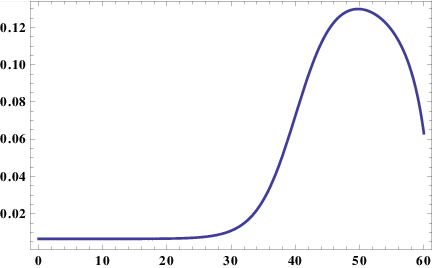


Example: axion quadratic model.—A similar phenomenon occurs in the axion–quadratic model discussed above. We plot the evolution of in Fig. . It exhibits three distinct components. The first is a negative spike, generated by the axion rolling off its hilltop. The second is a smaller positive spike produced by the axion rolling into its minimum. These two spikes come from the gauge contribution to , as clearly shown in Fig. . Fig. shows that each spike is inherited from a spike in the anisotropy factor. This is consistent with the analysis of Elliston et al. [32], in which the spikes were interpreted as due to strong deformations in the shape of the bundle. In the present interpretation, the differing signs arise because the principal curvature changes sign in the intermediate evolution.
As for the Byrnes et al. model, the intrinsic term does not respond immediately to this strong anisotropy, growing only later on approach to the adiabatic limit. The anisotropy is due to a strong shearing effect arising near the turn from dominantly -evolution to dominantly -evolution. Near the deep negative spike in , there is an enhancement in the shear oriented parallel to the principal isocurvature mode. This enhances the fluctuations in the isocurvature direction.
The third feature is the flat plateau at late times, associated with the adiabatic limit. Fig. shows that this comes from growth in the intrinsic term ; see the discussion in Refs. [65, *Kim:2011jea, 32].


VI Summary
In this paper we have developed an analogy between inflationary perturbation theory and geometrical optics. Here we summarize the main steps in the discussion.
Background.—In inflationary perturbation theory, we are interested in following the statistical properties—as measured by the correlation functions—of an ensemble of spacetime regions. This ensemble can be constructed equally well within the separate universe picture or traditional cosmological perturbation theory.
The ensemble picks out a cloud of points in phase space. In the limit , interactions between members of the ensemble are suppressed and each point moves along a phase space orbit of the unperturbed system. Therefore the ensemble traces out a narrowly-collimated “spray” or bundle of trajectories. Where slow-roll applies, the momenta are determined in terms of the fields and we can work in terms of a simplified flow on field space.
Optical quantities.—Geometrical properties of the bundle of trajectories can be used to describe its evolution and determine its statistical properties. The quantities of principal importance are obtained by decomposing the expansion tensor, yielding the dilation, shear and twist. These are well-known from the description of light rays in general relativity.
Jacobi fields and van Vleck matrix.—The dilation, shear and twist determine the evolution of Jacobi fields, which describe infinitesimal vectors connecting nearby trajectories. At any point in the flow, the van Vleck matrix aggregates the linearly independent Jacobi fields. The Jacobi fields themselves are measured from a fiducial trajectory, which can be thought of as the eikonal of geometrical optics. This analogy is exact within the slow-roll approximation.
We have argued that different implementations of the separate universe assumption—such as the Lyth–Rodríguez Taylor expansion, or the transport equations of §III—can be thought of as different methods to compute the Jacobi fields, in the form of the van Vleck matrix (16). More generally, the same is true for all approaches to perturbation theory in the limit . The most familiar implementation of the separate universe assumption, the “ formalism” or Taylor expansion approach, follows from Jacobi’s method of varying a solution with respect to its constants of integration. Conversely, the transport equations arise more naturally from Jacobi’s differential equation.
On approach to a caustic, some number of Jacobi fields decay. At an adiabatic caustic, defined in §II.4, all but one of the Jacobi fields decay. The single remaining field represents fluctuations along the caustic. In inflation this mode is the adiabatic fluctuation. The other Jacobi fields represent isocurvature fluctuations between the spacetime regions which make up the ensemble. Therefore, focusing at an adiabatic caustic can be interpreted as decay of isocurvature modes, or approach to an adiabatic limit in the sense of Elliston et al. [32].
Transport equations.—The “-tensors” encode evolution of the connecting vector fields. We have argued that these tensors can be computed using either cosmological perturbation theory or the separate universe approximation. More generally, any formalism which can reproduce the -space deviation equation (31) will reproduce the correct correlation functions, because the -tensors uniquely determine the transport equations. Therefore the -tensors may be used as an objective way to compare competing formalisms.
The transport equations obtained in this way are generalizations of the transport equations previously introduced in Ref. [17, *Mulryne:2010rp]. Because they are expressed in terms of -tensors, it follows that they can be integrated in terms of the Jacobi fields and their derivatives. Therefore the correlation functions can be expressed using the van Vleck matrix and its derivatives. (Technically it is the inverse of the van Vleck matrix which appears, in the form of the propagator matrix (15).)
In turn the van Vleck matrix can be expressed in terms of the integrated dilation, shear and twist. This makes it possible to diagnose regions where the flow may become adiabatic by tracking the behaviour of the focusing parameter , defined in Eq. (19), and the behaviour of the shear and twist.
Working within the slow-roll approximation we have argued that implies the presence of remaining isocurvature modes. To be compatible with experiment, these must almost certainly decay before the surface of last scattering. The consequent transfer of power into the adiabatic mode can change the value of .
Flow equations.—The Jacobi fields yield a formal solution for each correlation function, analogous to the “line of sight” used to simplify integration of the Boltzmann equation in CMB codes.
This formal solution demonstrates explicitly that the transport equations reproduce the Taylor expansion algorithm of Lyth & Rodríguez. In doing so we also obtain explicit expressions for the Taylor coefficients and in terms of integrals of the expansion tensor and its derivatives along the flow. Similar expressions had previously been obtained by Yokoyama et al. [14, *Yokoyama:2007dw].
These explicit expressions can be manipulated to obtain a closed set of evolution equations for the Taylor coefficients. These are Eqs. (37a) and (50). Such equations are extremely helpful in practice, because it means the Taylor coefficients can be obtained without the challenging problem of extracting a variational derivative after numerical integration: without a sufficiently accurate integration algorithm, the small variation of interest can be swamped by numerical noise.
Transport of shape coefficients.—Even after obtaining the Taylor coefficients, it is necessary to extract coefficients for each type of momentum dependence (or “shape,” in inflationary terminology) which occurs in a correlation function. An alternative is to return to the full -space transport equations and derive evolution equations for these coefficients directly. The first nontrivial case is the three-point function, whose shape coefficients are determined by Eq. (54).
Gauge transformations.—Specializing to the slow-roll approximation, where the flow can be described in field space, ray-tracing techniques can be used to obtain the gauge transformation to . In this way the gauge transformation is expressed using geometrical quantities in field space, rather than merely derivatives of the potential.
In models where a large is obtained from the gauge transformation, this gives a geometrical interpretation of its magnitude. The contributory factors are: (1) the -parameters of the adiabatic and principal isocurvature modes; (2) the principal curvatures of uniform-density hypersurfaces in field space; (3) the correlation coefficient between the adiabatic fluctuations and the fluctuations in each principal isocurvature mode; and (4) an anisotropy factor which measures distortions in the cloud of field-space points representing the ensemble.
In two cases where a large, transient contribution to has been observed, we show this principally arises from a strong enhancement in the anisotropy factor.
Comparison with other geometrical formulations.—In common with all other approaches to the evolution of correlation functions, the interpretation described in §§III–V is a reformulation of perturbation theory. All approaches carry the same physical content. Therefore, aside from practical considerations, the merit of each reformulation arises from the insight gained by emphasis on different structures.
The formulation we have given emphasizes the background phase space manifold, which encodes the structure of the theory in its geometry. This geometrical structure is mapped out by the behaviour of the trajectories flowing over it. Globally, this connection is made precise by the methods of Morse theory. Locally, it is encoded in the Jacobi fields whose role we have highlighted.
Attempts to reformulate perturbation theory in terms of geometrical objects have already attracted attention by various authors. Gordon et al. [86] and Nibbelink & van Tent [20] formulated perturbation theory for the two-point function in terms of the Frenet basis, which they called the “kinematical basis.” (See also Achúrcarro et al. [25].) Peterson & Tegmark later extended this approach to the three-point function [22, *Peterson:2010mv, *Peterson:2011yt]. A Frenet basis can be defined for each trajectory, and the Frenet–Serret equation describes how this basis is transported along the trajectory. In Refs. [86, 20, 22, *Peterson:2010mv, *Peterson:2011yt, 25] these equations are used to describe transfer between the adiabatic and isocurvature modes.
In the Frenet formulation, the isocurvature modes are identified with the normal, binormal, …, vectors. In our formulation these modes arise from the eigenvectors of the extrinsic curvature, , which we have described as the principal isocurvature modes. The tangent plane spanned by the Frenet normal, binormal, …, is the same as the subspace spanned by the eigenvalues of , so the physical content of these formulations is the same. More generally, in our formulation the properties of the isocurvature modes are expressed using the familiar mathematical apparatus used to describe hypersurfaces—normal vectors, first and second fundamental forms, and so on.
In addition, we explicitly separate a “local” contribution to each correlation function, arising from a gauge transformation and depending on the precise orientation of the Frenet basis, from the “integrated” contributions, obtained by solving the transport equations. Although it is clear that one can equally well express the integrated contributions in any suitable basis, it requires extra effort to rotate to the Frenet basis at each step in the integration. We feel it is preferable to express the evolution equations of perturbation theory in terms of the original basis on field space.
Future directions.—This formalism can be extended in several directions.
First, at some points in the discussion we specialized to the slow-roll approximation, to take advantage of certain simplifications—such as the twist-free and hypersurface-orthogonal character of flow. However, as we have presented it, the underlying formalism is independent of slow-roll. It can be used to evolve both field and momentum perturbations. This is desirable because future data from microwave background or galaxy surveys will be highly accurate, demanding commensurate accuracy in our theoretical calculations.
Second, in this paper we have interpreted the decay of isocurvature modes, and approach to an adiabatic limit, as focusing of the bundle to an “adiabatic” caustic. Our detailed discussion was restricted to field space. It should also be possible to study focusing and decay of isocurvature modes on the full phase space, providing a framework for the study of kinetically dominated scenarios, such as descent through the waterfall of hybrid inflation, where focusing may also occur.
Third, the existence of explicit expressions for the Taylor coefficients and may enable new analytic solutions to be found.
Finally, the entire formalism can be extended to higher -point functions. The case of principal interest is the four-point function. In contrast to the three-point function, this requires two shape parameters which determine and .
Acknowledgements.
DS was supported by the Science and Technology Facilities Council [grant numbers ST/F002858/1 and ST/I000976/1], and would like to thank the Harish-Chandra Research Institute, Allahabad, for their hospitality during the programme Primordial Features and Non-Gaussianities (December 2010) where an early version of this work was presented. JF was supported by the Science and Technology Facilities Council [grant number ST/1506029/1]. DJM was supported by the Science and Technology Facilities Council [grant number ST/H002855/1]. RHR was supported by Fundação para a Ciência e a Tecnologia through the grant SFRH/BD/35984/2007, and acknowledges a research studentship from the Cambridge Philosophical Society. We would like to thank Antony Lewis and Andrew Liddle for comments on a draft version of the manuscript.Appendix A Yokoyama et al. backwards formalism
In §IV.2 we presented integral formulae for the “” coefficients, Eqs. (49a)–(49b), and noted that essentially identical expressions had been presented by Yokoyama et al. [14, *Yokoyama:2007dw, *Yokoyama:2008by]. (However, Yokoyama et al. obtained their results by very different means.) Since their work is closely related to our own in content and outlook, we take this opportunity to review and extend their results.
Their aim is to develop evolution or “transport” equations (in our terminology) for objects closely related to observation, such as the derivatives —defined in section §V—and the parameter. They proceed as we do, first fixing a flat initial hypersurface. In our notation this is distinguished with lower case Roman indices. Unlike us, they also fix the final slice to be the precise time at which we wish to know the value of each observable quantity. In our notation this slice is labelled with Greek letters, and we obtain the matrices and as a function of it. Observables can be obtained after evaluating these functions at the time of interest. Instead, Yokoyama et al. consider intermediate flat slices between the initial and final slices, and express their answers as a function of the intermediate time. As we now explain, observables are to be obtained by setting this intermediate slice equal to the initial hypersurface.
For convenience we extend our index notation, and label quantities evaluated on the intermediate slice with upper case Roman indices. Yokoyama et al. introduce the quantity
| (85) |
where was defined in §V. is the derivative of the number of e-folds between an intermediate flat hypersurface and the final uniform density hypersurface, with respect to the field values on the intermediate slicing. Yokoyama et al. introduce a further quantity . Note that is not to be confused with the focusing parameter defined in the text, which is the exponential of the integrated dilation. and obey the autonomous transport equations
| (86) | |||||
| (87) |
Evaluating at the final hypersurface gives , which provides a boundary condition for the differential equation. One can then evolve backwards in time until we reach the initial slice. At this point will equal , which is the Taylor coefficient we set out to calculate. After this has been done, can be evolved forwards from the initial hypersurface with boundary condition .
We describe this as the “backwards” formalism, to be contrasted with the “forwards” formalism we have described in the text.
The introduction of these quantities is ingenious. Employing Eq. (71) together with Eq. (49b) yields
| (88) |
In turn this leads to
| (89) |
Therefore, can be evaluated with knowledge only of , and .
In performing this calculation, Yokoyama et al. traded a three-index object (either or , depending which formulation is in use) for two one-index objects, and . This involves fewer equations and therefore can be numerically advantageous.
Nevertheless, the backwards formalism has some disadvantages. First, because it computes only the Taylor coefficients, information about isocurvature modes is discarded. The evolution equations for and , or and , allow the isocurvature modes to be retained.
Second, to obtain information about the time-evolution of any observable it is necessary to recalculate and with multiple final times. Although the method yields , which is apparently related to the gauge transformation at an intermediate time, this is not quite correct. is defined for a fixed future rather than past boundary condition, and therefore gives information about a range of scales at a fixed time of observation, rather than a fixed scale at a range of final times. The past-defined objects required for the latter are automatically provided by the forwards formalism, meaning that multiple integrations are not required.
If the time of observation is known then the backwards formalism gives an efficient means to treat multiple scales at once.
To extend the backwards formalism to the trispectrum, one needs to separate the observables and . For this purpose and themselves would be required. Therefore, given the potential utility of this method, we conclude by extending it to include a backwards evolution equation for . As for the spectrum, this can be used to obtain information about and over a range of scales at a fixed time of observation. It still requires the solution for only a two-index object. The transport equation for can be shown to be
| (90) |
This is to be solved backwards from the final hypersurface where is equal to .
References
- [1] E. Komatsu et al. (WMAP Collaboration), Astrophys.J.Suppl., 192, 18 (2011), arXiv:1001.4538 [astro-ph.CO] .
- [2] “The scientific programme of Planck,” (2006), arXiv:astro-ph/0604069 [astro-ph] .
- [3] P. Ade et al. (Planck Collaboration), (2011), arXiv:1101.2022 [astro-ph.IM] .
- [4] V. Desjacques and U. Seljak, Class.Quant.Grav., 27, 124011 (2010), arXiv:1003.5020 [astro-ph.CO] .
- [5] A. A. Starobinsky, JETP Lett., 42, 152 (1985).
- [6] D. H. Lyth, Phys.Rev., D31, 1792 (1985).
- [7] M. Sasaki and E. D. Stewart, Prog.Theor.Phys., 95, 71 (1996), arXiv:astro-ph/9507001 .
- [8] D. S. Salopek and J. R. Bond, Phys. Rev., D42, 3936 (1990).
- [9] M. Sasaki and T. Tanaka, Prog.Theor.Phys., 99, 763 (1998), arXiv:gr-qc/9801017 [gr-qc] .
- [10] D. Wands, K. A. Malik, D. H. Lyth, and A. R. Liddle, Phys.Rev., D62, 043527 (2000), arXiv:astro-ph/0003278 [astro-ph] .
- [11] D. H. Lyth and Y. Rodríguez, Phys.Rev.Lett., 95, 121302 (2005), arXiv:astro-ph/0504045 .
- [12] G. I. Rigopoulos and E. P. S. Shellard, JCAP, 0510, 006 (2005), arXiv:astro-ph/0405185 .
- [13] G. I. Rigopoulos, E. P. S. Shellard, and B. J. W. van Tent, Phys.Rev., D73, 083521 (2006a), arXiv:astro-ph/0504508 .
- [14] S. Yokoyama, T. Suyama, and T. Tanaka, JCAP, 0707, 013 (2007), arXiv:0705.3178 [astro-ph] .
- [15] S. Yokoyama, T. Suyama, and T. Tanaka, Phys.Rev., D77, 083511 (2008), arXiv:0711.2920 [astro-ph] .
- [16] S. Yokoyama, T. Suyama, and T. Tanaka, JCAP, 0902, 012 (2009), arXiv:0810.3053 [astro-ph] .
- [17] D. J. Mulryne, D. Seery, and D. Wesley, JCAP, 1001, 024 (2010), arXiv:0909.2256 [astro-ph.CO] .
- [18] D. J. Mulryne, D. Seery, and D. Wesley, JCAP, 1104, 030 (2011a), arXiv:1008.3159 [astro-ph.CO] .
- [19] L. Amendola, C. Gordon, D. Wands, and M. Sasaki, Phys.Rev.Lett., 88, 211302 (2002), arXiv:astro-ph/0107089 [astro-ph] .
- [20] S. Groot Nibbelink and B. van Tent, Class.Quant.Grav., 19, 613 (2002), arXiv:hep-ph/0107272 [hep-ph] .
- [21] Z. Lalak, D. Langlois, S. Pokorski, and K. Turzyński, JCAP, 0707, 014 (2007), arXiv:0704.0212 [hep-th] .
- [22] C. M. Peterson and M. Tegmark, Phys.Rev., D83, 023522 (2011a), arXiv:1005.4056 [astro-ph.CO] .
- [23] C. M. Peterson and M. Tegmark, Phys.Rev., D84, 023520 (2011b), arXiv:1011.6675 [astro-ph.CO] .
- [24] C. M. Peterson and M. Tegmark, (2011c), arXiv:1111.0927 [astro-ph.CO] .
- [25] A. Achúcarro, J.-O. Gong, S. Hardeman, G. A. Palma, and S. P. Patil, JCAP, 1101, 030 (2011), arXiv:1010.3693 [hep-ph] .
- [26] A. Avgoustidis, S. Cremonini, A.-C. Davis, R. H. Ribeiro, K. Turzyński, et al., JCAP, 1202, 038 (2012), arXiv:1110.4081 [astro-ph.CO] .
- [27] J.-L. Lehners and S. Renaux-Petel, Phys.Rev., D80, 063503 (2009), arXiv:0906.0530 [hep-th] .
- [28] C. Ringeval, Lect.Notes Phys., 738, 243 (2008), arXiv:astro-ph/0703486 [astro-ph] .
- [29] J. Martin and C. Ringeval, JCAP, 0608, 009 (2006), arXiv:astro-ph/0605367 [astro-ph] .
- [30] I. Huston and K. A. Malik, JCAP, 0909, 019 (2009), arXiv:0907.2917 [astro-ph.CO] .
- [31] I. Huston and K. A. Malik, JCAP, 1110, 029 (2011), arXiv:1103.0912 [astro-ph.CO] .
- [32] J. Elliston, D. J. Mulryne, D. Seery, and R. Tavakol, JCAP, 1111, 005 (2011), arXiv:1106.2153 [astro-ph.CO] .
- [33] L. Boubekeur and D. Lyth, Phys.Rev., D73, 021301 (2006), arXiv:astro-ph/0504046 [astro-ph] .
- [34] D. H. Lyth, JCAP, 0606, 015 (2006), arXiv:astro-ph/0602285 [astro-ph] .
- [35] D. Seery, Class.Quant.Grav., 27, 124005 (2010), arXiv:1005.1649 [astro-ph.CO] .
- [36] D. Polarski and A. A. Starobinsky, Phys.Rev., D50, 6123 (1994), arXiv:astro-ph/9404061 [astro-ph] .
- [37] J. García-Bellido and D. Wands, Phys.Rev., D53, 5437 (1996), arXiv:astro-ph/9511029 [astro-ph] .
- [38] D. Wands and J. García Bellido, Helv.Phys.Acta, 69, 211 (1996), arXiv:astro-ph/9608042 [astro-ph] .
- [39] D. Langlois, Phys.Rev., D59, 123512 (1999), arXiv:astro-ph/9906080 [astro-ph] .
- [40] S. Hawking and G. Ellis, The Large scale structure of space-time (Cambridge University Press, 1973).
- [41] F. de Felice and C. Clarke, Relativity on curved manifolds (Cambridge University Press, 1990).
- [42] R. H. Ribeiro and D. Seery, JCAP, 1110, 027 (2011), arXiv:1108.3839 [astro-ph.CO] .
- [43] T. Battefeld and J. Grieb, JCAP, 1112, 003 (2011), arXiv:1110.1369 [astro-ph.CO] .
- [44] D. Seery and J. E. Lidsey, JCAP, 0509, 011 (2005), arXiv:astro-ph/0506056 [astro-ph] .
- [45] R. Sachs, Proc.Roy.Soc.Lond., A264, 309 (1961).
- [46] R. Penrose, in Perspectives in Geometry and Relativity, edited by B. Hoffman (Indiana University Press, Bloomington, Indiana, 1966) p. 259.
- [47] H. Fried, Green’s functions and ordered exponentials (Cambridge University Press, 2002) ISBN 9780521443906.
- [48] G. Rigopoulos, E. Shellard, and B. van Tent, Phys.Rev., D73, 083522 (2006b), arXiv:astro-ph/0506704 [astro-ph] .
- [49] G. Rigopoulos, E. Shellard, and B. van Tent, Phys.Rev., D76, 083512 (2007), arXiv:astro-ph/0511041 [astro-ph] .
- [50] F. Vernizzi and D. Wands, JCAP, 0605, 019 (2006), arXiv:astro-ph/0603799 [astro-ph] .
- [51] T. Battefeld and R. Easther, JCAP, 0703, 020 (2007), arXiv:astro-ph/0610296 [astro-ph] .
- [52] D. Seery and J. E. Lidsey, JCAP, 0701, 008 (2007), arXiv:astro-ph/0611034 [astro-ph] .
- [53] M. Visser, Phys.Rev., D47, 2395 (1993), arXiv:hep-th/9303020 [hep-th] .
- [54] C. DeWitt-Morette, Annals Phys., 97, 367 (1976).
- [55] C. DeWitt-Morette and T. Zhang, Phys.Rev., D28, 2503 (1983).
- [56] C. DeWitt-Morette, T. Zhang, and B. Nelson, Phys.Rev., D28, 2526 (1983).
- [57] D. H. Lyth, K. A. Malik, and M. Sasaki, JCAP, 0505, 004 (2005), arXiv:astro-ph/0411220 [astro-ph] .
- [58] G. Rigopoulos and E. Shellard, Phys.Rev., D68, 123518 (2003), arXiv:astro-ph/0306620 [astro-ph] .
- [59] S. Weinberg, Phys.Rev., D78, 123521 (2008), arXiv:0808.2909 [hep-th] .
- [60] S. Weinberg, Phys.Rev., D79, 043504 (2009), arXiv:0810.2831 [hep-ph] .
- [61] J. Meyers and N. Sivanandam, Phys.Rev., D83, 103517 (2011a), arXiv:1011.4934 [astro-ph.CO] .
- [62] J. Meyers and N. Sivanandam, Phys.Rev., D84, 063522 (2011b), arXiv:1104.5238 [astro-ph.CO] .
- [63] S. Dimopoulos, S. Kachru, J. McGreevy, and J. G. Wacker, JCAP, 0808, 003 (2008), arXiv:hep-th/0507205 [hep-th] .
- [64] S. A. Kim and A. R. Liddle, Phys.Rev., D74, 023513 (2006), arXiv:astro-ph/0605604 [astro-ph] .
- [65] S. A. Kim, A. R. Liddle, and D. Seery, Phys.Rev.Lett., 105, 181302 (2010), arXiv:1005.4410 [astro-ph.CO] .
- [66] S. A. Kim, A. R. Liddle, and D. Seery, Phys.Rev., D85, 023532 (2012), arXiv:1108.2944 [astro-ph.CO] .
- [67] J. L. Cardy, Scaling and renormalization in statistical physics (Cambridge University Press, 1996).
- [68] J. Silk and M. S. Turner, Phys.Rev., D35, 419 (1987).
- [69] L. Alabidi and D. H. Lyth, JCAP, 0605, 016 (2006), arXiv:astro-ph/0510441 [astro-ph] .
- [70] E. Calzetta and B.-L. Hu, Phys.Rev., D55, 3536 (1997), arXiv:hep-th/9603164 [hep-th] .
- [71] E. Calzetta and B. Hu, Phys.Rev., D61, 025012 (2000), arXiv:hep-ph/9903291 [hep-ph] .
- [72] P. R. Jarnhus and M. S. Sloth, JCAP, 0802, 013 (2008), arXiv:0709.2708 [hep-th] .
- [73] C. W. Gardiner, Handbook of stochastic methods: for physics, chemistry and the natural sciences, Springer Series in Synergetics, 13 (Springer, 2002) ISBN 3540616349.
- [74] J. Smidt, A. Amblard, C. T. Byrnes, A. Cooray, A. Heavens, et al., Phys.Rev., D81, 123007 (2010), arXiv:1004.1409 [astro-ph.CO] .
- [75] J. Fergusson, D. Regan, and E. Shellard, (2010), arXiv:1012.6039 [astro-ph.CO] .
- [76] D. H. Lyth and D. Seery, Phys.Lett., B662, 309 (2008), arXiv:astro-ph/0607647 [astro-ph] .
- [77] D. Seery, JCAP, 0711, 025 (2007), arXiv:0707.3377 [astro-ph] .
- [78] D. Seery, JCAP, 0802, 006 (2008), arXiv:0707.3378 [astro-ph] .
- [79] C. Lam, J.Math.Phys., 39, 5543 (1998), arXiv:hep-th/9804181 [hep-th] .
- [80] M. Dias and D. Seery, Phys.Rev., D85, 043519 (2012), arXiv:1111.6544 [astro-ph.CO] .
- [81] D. H. Lyth and I. Zaballa, JCAP, 0510, 005 (2005), arXiv:astro-ph/0507608 [astro-ph] .
- [82] K. A. Malik and D. Wands, Phys.Rept., 475, 1 (2009), arXiv:0809.4944 [astro-ph] .
- [83] C. T. Byrnes, K.-Y. Choi, and L. M. Hall, JCAP, 0810, 008 (2008), arXiv:0807.1101 [astro-ph] .
- [84] C. T. Byrnes, K.-Y. Choi, and L. M. Hall, JCAP, 0902, 017 (2009), arXiv:0812.0807 [astro-ph] .
- [85] D. Mulryne, S. Orani, and A. Rajantie, Phys.Rev., D84, 123527 (2011b), arXiv:1107.4739 [hep-th] .
- [86] C. Gordon, D. Wands, B. A. Bassett, and R. Maartens, Phys.Rev., D63, 023506 (2001), arXiv:astro-ph/0009131 [astro-ph] .