Creation of the CMB spectrum: precise analytic solutions for the blackbody photosphere
Abstract
The blackbody spectrum of CMB was created in the blackbody photosphere at redshifts . At these early times, the Universe was dense and hot enough that complete thermal equilibrium between baryonic matter (electrons and ions) and photons could be established on time scales much shorter than the age of the Universe. Any perturbation away from the blackbody spectrum was suppressed exponentially. New physics, for example annihilation and decay of dark matter, can add energy and photons to CMB at redshifts and result in a Bose-Einstein spectrum with a non-zero chemical potential (). Precise evolution of the CMB spectrum around the critical redshift of is required in order to calculate the -type spectral distortion and constrain the underlying new physics. Although numerical calculation of important processes involved (double Compton process, comptonization and bremsstrahlung) is not difficult with present day computers, analytic solutions are much faster and easier to calculate and provide valuable physical insights. We provide precise (better than ) analytic solutions for the decay of , created at an earlier epoch, including all three processes, double Compton, Compton scattering on thermal electrons and bremsstrahlung in the limit of small distortions. This is a significant improvement over the existing solutions with accuracy or worse. We also give a census of important sources of energy injection into CMB in standard cosmology. In particular, calculations of distortions from electron-positron annihilation and primordial nucleosynthesis illustrate in a dramatic way the strength of the equilibrium restoring processes in the early Universe. Finally, we point out the triple degeneracy in standard cosmology, i.e., the and distortions from adiabatic cooling of baryons and electrons, Silk damping and annihilation of thermally produced WIMP dark matter are of similar order of magnitude ().
Keywords
cosmic background radiation, cosmology:theory, early universe1 Introduction
There are several important events in the history of the Universe which provide the foundations for the standard cosmological model. The first event is the big bang, which created the present expanding Universe filled with matter, radiation and dark energy. One of the goals of cosmology is to reconstruct these initial conditions and learn about the high energy physics at early times. We should emphasize here that the blackbody spectrum of cosmic microwave background (CMB) is not an initial condition. The blackbody spectrum is created and maintained dynamically throughout the early history of the Universe () by standard physics processes and how this happens is the main topic of the present paper. The CMB spectrum thus provides information about the physics of the Universe after the big bang.
The other important events in standard cosmology are: the formation of light elements in primordial nucleosynthesis (1), recombination of electrons and ions to neutral atoms (2, 3), and reionization of the Universe (4) by the radiation emitted by first stars and galaxies. We should also mention electron-positron annihilation at which more than doubles the entropy of CMB and raises its temperature by . The important events in the history of the Universe are sketched in Fig. 1. Big bang nucleosynthesis (BBN) theory together with measurement of light elements abundances constrains the photon to baryon number density at (see 5, for a review) and is the earliest direct evidence and measurement of electromagnetic radiation in the early Universe. The fact that the photon energy density inferred from BBN and Cosmic microwave background (CMB) at (6) are close to each other (consistent within ) also implies that we do not have arbitrary freedom in adding energy to CMB between these two epochs. There is, however, no direct way to constrain the energy density in photons before BBN and the epoch of electron-positron annihilation.
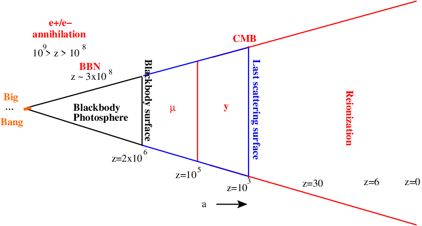
The CMB (anisotropy and polarization) is at present the most precise cosmological probe. The CMB spectrum was created at , and this critical redshift defines the blackbody surface for our Universe. Spatial fluctuations in the temperature of the CMB were imprinted much later, when the electron and protons recombined to form hydrogen atoms at . This second boundary defines the well known last scattering surface, the structure of which is encoded in the photon visibility function (7, first studied by). The anisotropies and physics at the last scattering surface have been very well studied and accurate analytic (8) and numerical solutions (9, 10) have been available for some time, motivated by the precise experiments such as WMAP (6) and Planck (11).
The blackbody spectrum, once created at high redshifts (for example before the time of electron-positron annihilation), is preserved by the adiabatic expansion of the Universe at all subsequent times. However, if there is energy release at lower redshifts , for example by particle decay and annihilation or Silk damping, it will distort the CMB spectrum away from the Planck form. In this case, Zeldovich and Sunyaev (12) first demonstrated that bremsstrahlung alone cannot recreate blackbody spectrum until very high redshifts, almost up to the time of electron-positron annihilation. The problem of evolution of the CMB spectrum through the blackbody surface, in the presence of heating, was solved analytically by (13) including the processes of comptonization and emission and absorption of photons with special emphasis on bremsstrahlung. Comptonization is the process of redistribution of photons over frequency, resulting from the Doppler and recoil effects of Compton scattering of photons on thermal electrons (14). Since the double Compton cross section (15, 16) has a dependence on frequency similar to bremsstrahlung, the solution of Sunyaev and Zeldovich (13) also allowed inclusion of double Compton emission and absorption, which is dominant over bremsstrahlung in a low baryon density Universe such as ours and was first considered by (17). Double Compton emission or absorption is just the first radiative correction to the process of Compton scattering just as bremsstrahlung is the first radiative correction to the scattering of electrons on nuclei (18, see discussion in ). The approximations used in these analytic solutions result in accuracy of at redshifts () and worse than at higher redshifts. Much better accuracy is, of course, achievable in numerical solutions (19, 20, 21, 22, 23).
The type of spectrum we get for the CMB is determined by the Compton parameter, defined in Eq. (5). Bose-Einstein spectrum can be created only at high redshifts (7), when comptonization of CMB is very efficient. Any addition of energy and photons to CMB at inevitably distorts the CMB spectrum with a -type distortion (12). The -type distortions, in contrast to -type distortions, can be created at low redshifts up to . Reionization at in particular is expected to create -type distortions of magnitude where is the optical depth due to reionization, is the average temperature during reionization, is the Boltzmann’s constant, is the speed of light and is the mass of electron. Due to uncertainties in reionization physics, it will be extremely difficult to separate these low redshift distortions from the -type distortions created before recombination. COBE FIRAS experiment (24) measured the CMB spectrum with high precision and placed a constraint on the chemical potential of Bose-Einstein spectrum for CMB of , thus confirming that the CMB has a Planck spectrum at very high accuracy.
In standard model of cosmology we can get constraints on the energy density of radiation from two distinct and very precise observables. The first is the deuterium abundance, which gives the baryon number to photon number ratio during primordial nucleosynthesis at (25, 5). The second is the measurement of CMB anisotropies, which constrains the baryon to photon ratio (6) during recombination at . The fact that these two values of baryon to photon ratio are almost identical with small error bars means that we do not have arbitrary freedom in adding energy to CMB, for example, with the introduction of new physics. In fact any addition of energy/entropy to CMB between primordial nucleosynthesis and recombination cannot be more than a small percentage () of the photon energy density during BBN.
In standard cosmology, the chemical potential of CMB is expected to have a magnitude of resulting from the heating of CMB by Silk damping. A similar magnitude but opposite sign distortion, , is expected from cooling of photons due to energy losses to baryons and electrons, which have a different adiabatic index (5/3) than radiation (4/3) and as a result cool faster than the radiation as the Universe expands (23, 26). A detection of a chemical potential of magnitude greater than will therefore mean existence of non-standard physics (or a small scale power spectrum that is bigger than what is expected from extrapolating the large scale power spectrum as measured by CMB and large scale structure) at these redshifts. Proposed experiment Pixie (27) has exactly this level of sensitivity. Constraining high energy physics using -type distortions requires precise calculation of evolution of the CMB spectrum through the blackbody surface at . Analytic solutions provide valuable physical insight in addition to being much easier to compute. Motivated by these factors we try to improve the method of (13) to achieve better than precision in analytic solutions. These solutions should prove useful in predicting the signal from models of high energy physics which can provide energy injection to CMB at these high redshifts.
In the last part of the paper we apply our analytic solution to examples from the standard model of cosmology including electron-positron annihilation and dark matter annihilation. These simple examples in particular demonstrate the efficiency of processes responsible for maintaining thermal equilibrium in the early Universe. They also demonstrate the difficulty of creating spectral distortion in CMB at high redshifts. There remains thus only a narrow window at redshifts when a Bose-Einstein spectrum can be created.
We use WMAP (6) best fit parameters for cosmology for numerical calculations.
2 Thermalization of CMB
Compton scattering is responsible for creating a Bose-Einstein spectrum of photons if the rate of comptonization (i.e. the redistribution of photons over the entire spectrum by Compton scattering) is greater than the expansion (Hubble) rate of the Universe (12). This condition is satisfied at redshifts . In the non-relativistic regime comptonization is described by Kompaneets equation (14). Compton scattering, however, conserves photon number and therefore the spectrum obtained as a result of comptonization will in general have a non-zero chemical potential. At redshifts double Compton scattering, and to a lesser extent bremsstrahlung, can emit/absorb photons at low frequencies very efficiently because the optical depth and the absorption coefficient of these two processes increase with decreasing frequency as . Compton scattering is then able to redistribute these photons over the entire spectrum. The net result is that the chemical potential is exponentially suppressed and a Planck spectrum is established.
The equilibrium electron temperature in a radiation field with occupation number , where and is the temperature of reference blackbody, is given by (28, 29)
| (1) |
The rate () at which electron/baryon plasma achieves equilibrium temperature given by Eq. (1) is shown in Fig. 2 in the topmost curve. Rates of bremsstrahlung absorption , double Compton absorption and Compton scattering are also compared with the Hubble rate in Fig. 2. is the electron number density, is the Thomson cross section, is the electron temperature, is the number density of ions, is the dimensionless frequency corresponding to frequency , is the Planck’s constant, is the energy density of photons. , and blackbody spectrum is assumed for this figure. The rate coefficients are given by:
| (2) | ||||
| (3) | ||||
| (4) |
is the fine structure constant and is the baryon number density. for a blackbody spectrum at temperature , is the baryon density parameter, is the Hubble parameter and is the primordial helium mass fraction. is the average gaunt factor for bremsstrahlung, is the number density of ion species and the charge of ion. The sum is over all ionic species, which for the primordial plasma at high redshifts consists of protons and helium nuclei. Accurate fitting formulas for have been provided by (30). is the gaunt factor for double Compton scattering and accurate fitting formula for it has been calculated recently by (23). We use these fitting formulae for numerical solution. For reference at , and and we use these values for our analytic solutions. These gaunt factors are slowly varying functions of time and frequency and can be assumed to be constant in the redshift range of interest for analytic calculations. We justify this assumption below.
The division into -type and Bose-Einstein regions depends on the Compton parameter,
| (5) |
During radiation domination () the integral can be carried out analytically, giving , where is the redshift when matter energy density equals radiation energy density and we have assumed effective species of massless neutrinos (31). We have, for WMAP cosmological parameters (6), , and . For we have a -type distortion and for a Bose-Einstein spectrum. The spectrum attained for is in between a pure -type and Bose-Einstein. We choose as an approximate division between the two types of distortions for our estimates. This division is accurate if the energy injection between is small compared to the total energy injection at . If most of the energy injection happens between , then numerical calculations must be performed to get accurate final spectrum. We note that for small distortions, we can calculate distortions arising from different physical processes separately and add them linearly.

2.1 Kinetic equation
We will follow (13) in solving the kinetic equation for photon distribution using stationarity assumption and then do an iteration to relax this assumption to arrive at a more accurate solution. The kinetic equation for the evolution of photon occupation number in the presence of Compton scattering, double Compton scattering and bremsstrahlung is given by (20, 21, see also)
| (6) |
The first term with coefficient is the Kompaneets term describing Compton scattering. The three terms in the square brackets in Kompaneets term describe photon diffusion in frequency due to the Doppler effect, electron recoil and induced recoil effects respectively. The second term represents emission and absorption of photons due to double Compton () and bremsstrahlung (). The last term in Eq. (6) arises because we are evaluating the time derivative at constant instead of constant frequency , and electron temperature changes with time11 1 This is in addition to the usual dependence due to the expansion of the Universe. The variable is invariant w.r.t. the expansion of the Universe. because the photon distribution is evolving (see Eq. (1)).
We are interested in the regime where comptonization is efficient and deviation from a Planck spectrum is small. In this regime the photon spectrum is described by a Bose-Einstein distribution with a chemical potential much smaller than unity in magnitude.
| (7) |
The total energy density and number density of photons is then given by 22 2 The chemical potential is not constant but a function of frequency at low frequencies but this dependence is important only for calculating the photon production rate. We can ignore the frequency dependence in calculating the total energy and number density in the spectrum since the contribution from low frequencies () to these quantities is small and the constant assumption introduces negligible error.
| (8) | ||||
| (9) |
where is the radiation constant, , is the Riemann zeta function with , ,, and .
In order to cancel the effect of the expansion of the Universe we will use the blackbody spectrum with temperature , is its energy density and its number density. If we have a source injecting energy density at a rate and photon number density at rate , where , , we get using Eqs. (8) and (9) and with
| (10) | ||||
| (11) |
For small distortions and we have at lowest order, and . The photon production due to double Compton and bremsstrahlung can be calculated by taking the time derivative of Eq. (9). Multiplying the kinetic equation Eq. (6) by and integrating over and using it in the the time derivative of Eq. (9), the terms involving cancel out and only the bremsstrahlung and double Compton terms contribute, giving
| (12) |
In general there may be additional sources of photons, for example, if energy is injected as an electromagnetic shower resulting from decay of a heavy particle, the resulting cascade may produce non-negligible amount of photons. However in most cases of interest and at high redshifts this is much smaller than the photon production from bremsstrahlung and double Compton.
2.2 Numerical solution
In order to calculate the precision of the analytic formulae derived below, we compare them with the numerical solution of the coupled system of Eqs. (6) and (1). The initial spectrum for the numerical solution is a type distortion of magnitude at with the chemical potential decaying exponentially with decreasing frequencies at (see Eq. (14) below). The results are not sensitive to the exact form of initial spectrum if the starting redshift is , what matters is the total energy input into an initial blackbody. We solve equation (6) iteratively in small time steps (using Compton parameter as the time variable) of . In the first iteration we use the analytic solution for the evolution of electron temperature. In the second iteration we use the solution of first iteration to calculate the electron temperature using Eq. (1). As a frequency variable we use a where is the reference temperature which evolves just by redshifting due to cosmological expansion and is equal to the electron temperature at the start of each iteration step. This gets rid of the last term in Eq. (6) and introduces factors of in the Kompaneets and bremsstrahlung/double Compton terms. We also write the total spectrum as a sum of blackbody part at reference temperature and a distortion part, keep only the terms linear in distortions and solve the linearized Eq. (6) for distortions, as the zeroth order blackbody part vanishes. Implicit backward differentiation method is used to solve the PDE. We use logarithm of as the second independent variable with the variable step size in the direction.
The main source of error is the deviation of electron temperature used in solving the PDE from the correct temperature given by Eq. (1), resulting in violation of energy conservation. In our solution, the maximum error in energy conservation as a fraction of energy in the distortion occurs at high redshifts, when there is strong evolution of , but even this is in each iterative step. The error with respect to the total energy density in photons is, therefore, , since we start with an initial distortion of , and is much smaller in the later steps as the distortion decays exponentially. An important point to note here is that since we change the reference temperature to the current electron temperature at the beginning of each iterative step, and solve and track only the distortion part, the error in in individual iterative steps does not accumulate but is in fact suppressed in the subsequent evolution of the spectrum by the visibility factor (defined below). The solution obtained can thus be considered almost exact for the purpose of the present paper.
The high frequency spectrum is forced to be Wien at with the chemical potential and temperature given by analytic solution. The low frequency boundary is at and the spectrum at is forced to be blackbody with the temperature equal to the analytic electron temperature. Since our boundaries are far away in the distant Wien/Rayleigh-Jeans tails, where there are negligible amount of photons/energy , the solution is not sensitive to the exact boundary conditions. Since our boundary conditions are approximately equal to the true solution, we are able to use large steps in the direction resulting in considerable speedup in the numerical calculation compared to a calculation with arbitrary (but reasonable) boundary conditions. The initial spectrum is evolved until recombination () although the distortion at is effectively frozen-in after . Further details on numerical issues can be found in [20, 22, 23].
3 Solution using stationarity approximation
In order to calculate the integral in Eq. (12) we need to know the occupation number . Note that we cannot use Bose-Einstein distribution as an approximation since the integral in this case diverges at small . The reason is that double Compton and bremsstrahlung rates diverge at small frequencies and establish Planck spectrum. We can get an approximate solution from the kinetic equation Eq. (6) (14) by assuming that the instantaneous spectrum is stationary. Thus, neglecting time derivatives, making chemical potential function of frequency,33 3 We note that any spectrum can be described by a frequency dependent chemical potential. , and also assuming, Eq. (6) simplifies considerably,
| (13) |
The solution of this ordinary differential equation with the boundary condition is given by (13)
| (14) |
where is normalization specified by chemical potential at large . Thus decays exponentially at small frequencies and goes to constant at large frequencies. is also the frequency at which comptonization rate is equal to photon absorption rate due to double Compton and bremsstrahlung. Similarly we can also define a frequency at which the photon absorption rate is equal to the Hubble rate (21),
| (15) |
and are plotted in Fig. 3. We note that in the redshift range of interest. This is consistent with assumptions made in the derivation. Also, since in the redshift range of interest and gaunt factors are slowly varying functions of frequency and temperature, we can assume and .
We should emphasize that the sole purpose of finding an accurate solution for the spectrum at low frequencies is to calculate precisely the photon emission/absorption due to bremsstrahlung and double Compton. In particular, only the spectrum at is frozen-in at . The low frequency spectrum continues to be affected by bremsstrahlung (at smaller redshifts, during recombination and after), which tries to bring the spectrum in equilibrium with the electrons, which are cooler than the radiation due to adiabatic expansion (23, 26). Furthermore, most of the photons are created around the critical frequency . The double Compton gaunt factor at the critical frequency deviates from the value by less than in the interesting redshift range of . The bremsstrahlung gaunt factor has a maximum deviation of from in the same redshift range, but since it is only a small correction to the dominant double Compton process, the error in the final solution for evolution is small. Thus the assumption of constant gaunt factor is an excellent one for the present problem and is further justified by a comparison of the analytic and numerical solutions.

We can now use the solution Eq. (14) to evaluate the integral Eq. (12) (ignoring the dependence of gaunt factors),
| (16) |
Equations (10) and (11) along with the above solution give the following equation for the evolution of chemical potential at ,
| (17) |
where , . are the extra photons injected from processes other than the low frequency bremsstrahlung and double Compton photons calculated above, for example, from the same source which injects energy. We assume this extra term to be negligible in the rest of the paper. The solution of Eq. (17) at is given by
| (18) |
where , is the initial/maximum energy injection redshift and we have defined the effective blackbody optical depth (which is frequency independent at )
| (19) |
where
| (20) |
is the total radiation density parameter, and is the Hubble constant today. It is interesting to note that in the absence of double Compton scattering we would have . The presence of double Compton increases the critical frequency from its bremsstrahlung only value, and thus reducing the bremsstrahlung emission. It is also straightforward to calculate, if needed, the chemical potential at any intermediate redshift using Eq. (18) by replacing (and similarly for ) with and also replacing the lower limit in the integral with ,
| (21) |
The solution given in Eq. (14) corresponds to Eq. (15) in (13) but including the double Compton process. Similarly, the solution in Eq. (19) generalizes Eq. (20) of (13). The dominant term ()in Eq. (19) is due to the double Compton process with the bremsstrahlung term () providing a small but important correction.
4 Improved solution by approximating non-stationarity using previous solution
We will see below that the solution arrived at in the previous section underestimates the photon production. It turns out that the stationary solution, which is normalized at high frequencies, underestimates the chemical potential at small frequencies where most of the photons are being produced/absorbed. We find below the correction for the normalization of chemical potential, which enables us to improve the formula for blackbody optical depth Eq. (19) in the solution Eq. (18). The result of the computations, using the new analytic formula Eq. (26) for the blackbody optical depth, deviates from numerical solution by less than .
A very simple correction to the normalization can be arrived at as follows. An immediate improvement over the solution of (13) is possible by approximating the non-stationarity in Eq. (13) using the solution Eq. (17) (ignoring the energy injection term)44 4 The energy injection term will add a inhomogeneous term to the homogeneous equation for . The effect of this term is to change the overall normalization without significantly affecting the shape of the spectrum. This term can therefore be neglected for the purpose of calculating the photon creation/absorption.
| (22) |
Note that the time derivative of temperature in Eq. (6) can be neglected at small frequencies as its effect is suppressed by a factor of with respect to the term with the time derivative of . Equation (13) with the above approximation for the non-stationary term gives Bessel’s equation
| (23) |
The solution is given in terms of modified Bessel function of second kind ,
| (24) |
This result provides a more precise dependence of on frequency compared to Eq. (14). Choosing normalization to give at gives , where this fit is accurate for . This fit thus covers all the interesting range for critical frequency (see Fig. 3). This choice of normalization frequency () provides a good fit to the numerical solution.
The normalization frequency is chosen so that (i) it is , since this is the assumption made in deriving the analytic solution and (ii) it is also large enough so that . Since we only want to use this solution to calculate the total photon emission, it need only be accurate at . The only requirement at is that its contribution to the photon emission/absorption should be negligible at and that it should be approximately constant around , as expected from a correct solution. We should also point out that decreases with increasing at for the solution in Eq. (24) and . Thus our solution satisfies the requirements outlined above. Obviously it cannot be normalized at , as was done with the original solution Eq. (14). The normalization must be done by comparison with the numerical solution, taking into account the assumptions made in arriving at this solution, resulting in our choice of .55 5 Since is approximately constant around (variation in the analytic solution is less than for ), the exact value of normalization frequency is not important, and we get similar precision if we choose to normalize at a slightly different frequency around , for example at . We should also mention that the numerical solution also shows a tiny decrease ( from to ) in the chemical potential at because of the increasing efficiency of the recoil effect at high frequencies. We show a snapshot of the numerical solution (chosen at random) at , original solution Eq. (14) and improved solution Eq. (24) in Fig 4. The critical frequency at this redshift is . Needless to say that the shape of the spectrum is well described by our solution at all redshifts and we have chosen a random snapshot in Fig. 4 for illustration. The final justification for all our assumptions and approximations is of course given by a comparison of the final numerical and analytic solutions for the evolution of the chemical potential with redshift as described below.

We can now use our improved solution to calculate the photon production rate
| (25) |
Proceeding as before we get improved formula for blackbody optical depth,
| (26) |
where we have defined
The improved solution for evolution of is still given by the original equation (18) on substituting the improved optical depth given by Eq. (26).
The improved solution has a broad region of validity and covers the entire redshift range of interest. The physics used to derive Eq. (26) is applicable for redshifts . Thus we can use the blackbody optical depth, Eq. (26), for redshift interval , the upper limit is well behind blackbody surface at . At the number density of positrons becomes comparable to the number density of electrons/baryons due to pair production. At higher redshifts, the number density of electrons and positrons, and thus the rates of Compton scattering, double Compton and electron-electron and electron-positron bremsstrahlung, increase exponentially with increasing redshift. Thus the blackbody optical depth, also starts increasing exponentially instead of a power law as in our solution and Eq. (26) is no longer applicable. However, we already have at , and creation of a distortion in photon spectrum is thus impossible at higher redshifts.
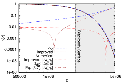
We plot the optical depth for the numerical solution, the total improved solution as well as the individual terms in Eq. (26) in Fig. 5. At high redshifts, double Compton terms dominate with the new double Compton term also contributing. Bremsstrahlung term becomes important at low redshifts. At high redshifts, our improved solution is indistinguishable from the numerical solution. As blackbody optical depth becomes small the quasi-static assumptions made in arriving at the analytic solution also breakdown and the error grows. The new solution is however an excellent approximation to the numerical result, and definitely better than the double Compton only result, over the entire redshift range of interest, where the optical depth is greater than a few . The deviations from the numerical result for the double Compton only formula and our new result are plotted in Fig. 6. The analytic solution overestimates the photon production at low redshifts. The reason becomes clear by looking at in Fig. 3. Photon production at would be suppressed since the photon production rate is smaller than the expansion rate. At high redshifts, and the error introduced by including is negligible since photon production is negligible at these frequencies anyway. At low redshifts, becomes less than unity and starts approaching and Eqs. (16) and (25) overestimate photon production. We show the blackbody visibility factors66 6 This is really the visibility of distortions. When the visibility is small, the distortions are not visible, and when the visibility is unity, distortions survive and are visible today. in Figs. 7 and 8 for analytic solution Eq. (26), for the double Compton only term and the numerical result. The accuracy of blackbody visibility is better than with the new solution Eq. (26).


5 Examples from standard cosmology
5.1 Upper limit to energy release after BBN and before recombination
In standard model of cosmology, we can get constraints on energy density in radiation from two distinct and very precise observables. The first is the deuterium abundance, which gives the baryon number to photon number ratio during primordial nucleosynthesis at (25, 5). The second is the measurement of CMB anisotropies, which constrains the baryon to photon ratio (6) during recombination at . The fact that these two values of baryon to photon ratio are almost identical, with small error bars means that we do not have arbitrary freedom in adding energy to CMB, for example, with the introduction of new physics. In fact any addition of energy/entropy to CMB between primordial nucleosynthesis and recombination cannot be more than a small percentage ( for CMB and BBN to be consistent within ) of the already existing radiation energy density. COBE limit (24) of implies that a energy can be added only at redshifts . These limits also justify our assumption of small distortions in the analytic calculations. Any energy injection into photons from non-standard processes before electron-positron annihilation, however, is unconstrained.
5.2 Electron-positron annihilation
It is, of course, possible to add of order unity energy to radiation before primordial nucleosynthesis. This happens in standard cosmology during electron-positron annihilation (32, 33, 34), which more than doubles the energy density of photons and increases their temperature by . In the early stages of electron-positron annihilation, the electrons/positrons far outnumber the photons. In this era, therefore, electron-positron annihilation and electron-electron/electron-positron bremsstrahlung dominate the thermalization process. In the very late stages, when most of the electron-positrons have annihilated, Compton and double Compton scattering are dominant, electron number is conserved and their density evolves according to the non-relativistic adiabatic law, and our analytic formulae become applicable. We, of course, do not expect any observable distortion from electron positron annihilation (13). It is still interesting to calculate the magnitude of the distortion to demonstrate the effectiveness of double Compton scattering and comptonization in restoring the equilibrium between matter and radiation.
At redshifts , most of the positrons have annihilated and their number density falls below that of electrons. The number density of electrons is high enough (as a result of asymmetry in matter anti-matter) to maintain the annihilation rate much faster than the expansion rate. We can, thus, use Saha equation to follow the positron number density during the last stages of positron annihilation. Using the fact that the positron number density is much smaller than the electron number density and that the electron number density is unaffected by annihilation, we get for the positron number density ,
| (28) |
where the equilibrium (zero chemical potential) number density of electrons/positrons is
| (29) |
The rate of energy injection is given by,
| (30) |
We have plotted the resulting injection rate multiplied by redshift, in Fig. 9. Visibility function suppresses the high redshift contribution, while the exponentially decreasing positron number density suppresses the low redshift contribution, giving the peak at . The chemical potential from electron-positron annihilation is suppressed by an astronomical factor of ! Thus it is impossible to create a deviation from blackbody spectrum at high redshifts.

5.3 Primordial nucleosynthesis
Big bang nucleosynthesis (BBN) at results in binding of almost all neutrons into helium () along with the production of small amount of deuterium (), helium-3 , tritium , beryllium-7/lithium-7 (), lithium-6 () and trace amounts of heavier elements (see 35, for a recent calculation). We can get a rough estimate of the energy released during this main part of nucleosynthesis by calculating the total binding energy of helium-4 produced.77 7 We ignore the fact that some of the energy will be lost to neutrinos. Thus we have an energy release of . The blackbody optical depth at is and we have the final . However, tritium and beryllium-7 survive for a long time before decaying into helium-3 and lithium-7 respectively. Although, the energy released in the decay of beryllium-7 and lithium-7 is much smaller than that released during helium production in BBN, the distortions are much larger because these decays happen in front of the blackbody surface, when the blackbody visibility is almost unity. Also, the energy density released is proportional to the number density of beryllium-7 and lithium-7, which has decreased as compared to the decrease of the radiation energy density, thus giving a larger than if the decay had happened at the same time as the main BBN. Tritium has a half life of years. It, therefore, decays at to helium-3 releasing an electron with average energy KeV. Most of this energy release happens at and causes a -distortion with .
Neutral beryllium atom decays by electron capture with a half life of 53.2 days. Fully ionized beryllium in the low density plasma in the early Universe is however stable. It has to wait for years until when it recombines to hydrogen like beryllium. The recombined beryllium can now capture the orbital electron and decay to lithium-7 with a half-life of 106.4 days, which is twice the half-life of a fully recombined beryllium (36). of the decays go to the ground state of lithium-7 and most of the energy released is carried away by neutrinos, which would appear today as a narrow line in the cosmic neutrino spectrum. of beryllium decays into an excited state of lithium. About half of the total decay energy in this case also is lost to neutrinos forming a second lower energy line in the cosmic neutrino spectrum. The excited lithium nucleus then de-excites, almost immediately, to the ground state, emitting a KeV photon, which delivers most of its energy to plasma by Compton scattering on electrons (recoil effect). The Compton parameter at is , which lies intermediate between pure and type eras. The heating, therefore, results in a distortion intermediate between the and the type distortions of magnitude (using formula for -type distortion) .
5.4 Dark matter annihilation
A natural and favored candidate for dark matter is a weakly interacting massive particle (WIMP) with several candidates in high energy theories beyond the standard model (37). A very attractive feature of WIMP is that if they have weak scale interactions then the correct amount of dark matter (which is close to the critical density) observed today can be thermally produced in the early Universe. This is remarkable since a priori there is no reason to suspect any relation between the weak scale interactions and the present critical density of the Universe and this coincidence is sometimes referred to as the WIMP miracle. For the thermally produced WIMPs, the dark matter density is related to the velocity averaged cross section as
| (31) |
where is the Hubble parameter and is the dark matter density as a fraction of critical density today. The above values for annihilation cross sections are of similar order of magnitude as the current upper limits from Fermi-LAT experiment probing dark matter annihilation in the local Universe (38, 39, 40). The actual annihilation cross section can, of course, be much smaller than the Fermi upper limits. Energy released from dark matter annihilation also changes recombination history (41) and it can thus be constrained through its effect on the CMB power spectrum (42, 43) and recombination spectrum (44). Effect of dark matter annihilation also changes the abundance of elements produced during BBN (45, 46); these constraints are complementary but less stringent compared to the current CMB constraints.
Initially, dark matter is in thermal equilibrium with other constituents of the Universe, and is being continuously created and annihilated. As the Universe cools and expands, these interactions freeze out and thereafter the dark matter number is conserved. However, a small number of residual annihilations keep happening throughout the history of the Universe. The rate of energy released into CMB from these residual annihilations88 8 We assume self annihilating Majorana particles. For Dirac particles the energy release would be smaller by a factor of 2. is given by,
| (32) |
where is the mass of the dark matter particle and is the fraction of energy that goes into particles with electromagnetic interactions, and is deposited in the plasma.
We plot the rate of energy release into the CMB
| (33) |
in Fig. 10 for the fraction of energy going into the plasma99 9 In general we expect some energy to be lost to neutrinos and other dark particles and therefore would be less than unity. . Hubble rate is proportional to during radiation domination, which gives us the flat portion of the curve. Energy release rate decreases faster than the expansion rate during matter domination, giving the low redshift declining tail in the plot. The total distortion (using energy release from ) is . The - type distortion from energy release is , these distortions were also calculated by (23). These numbers are of similar order of magnitude as the distortions from Silk damping and Bose-Einstein condensation of CMB discussed in the next two sections. COBE constraint of (24) constrains WIMP mass to be while PIXIE (27) would be able to constrain up to .

5.5 Silk damping
Sound waves are excited in the primordial baryon-electron-photon plasma by primordial perturbations. They decay on small scales because of shear viscosity, with thermal conduction also becoming important near the time of recombination. This damping of primordial perturbations was first calculated by Silk (47) including only thermal conduction. The full calculation, including both shear viscosity and thermal conduction and also including the effects of photon polarization was done by Kaiser (48). Silk damping transfers energy from sound waves to the average CMB spectrum, resulting in effective energy injection into CMB (49, 50, 51, 23, 52). Microscopically, shear viscosity and thermal conduction arise due to the diffusion of photons which are repeatedly scattered by the electrons. This diffusion of photon results in mixing of blackbodies from different phases of the sound waves on diffusion scales. of the dissipated energy in sound waves just increases the average temperature of CMB while results in the spectral distortions of and type. Depending on the primordial perturbation power spectrum at these very small scales of comoving wavenumbers , the distortion can be in the range (52) for the parameter space allowed in the standard cosmological model (6). We refer to (52) for a detailed discussion, including fitting formulae for spectral distortions from adiabatic initial conditions, and constraints from the future experiments on initial power spectrum spectral index and its running.
5.6 Bose-Einstein condensation of CMB
After the epoch of electron-positron annihilation, electrons and baryons are non-relativistic and cool adiabatically (with adiabatic index ) as a result of the expansion of the Universe, . Radiation (photons) has adiabatic index and cools slower than baryons, (2). Comptonization however is very efficient before recombination and efficiently transfer energy from photons to electrons/baryons, keeping them at same temperature as photons. This cooling of CMB (23), along with thermalization from comptonization, results in Bose-Einstein condensation of CMB (26). The photons thus move from high to low frequencies where they are efficiently destroyed by bremsstrahlung (and at high redshifts also by double Compton scattering). Since the amount of cooling is small, linear theory for small distortions applies. The resulting distortions have the same shape as that caused by heating of CMB in previous examples, but with opposite sign. Thus we have negative and negative distortions which partially cancel the distortions due to dark matter annihilation and Silk damping. Surprisingly, the (and ) distortions have a magnitude which is similar to those from dark matter annihilation and Silk damping. A comparison of distortions from Bose-Einstein condensation as well as all previous examples is presented in Table 1. We also show comparison of -type distortions in Table 2. -type distortions are dominated by the low redshift contributions, during and after reionization, from the intergalactic medium and clusters. Early universe physics is therefore difficult to constrain using the -type distortions.
| Process | |
|---|---|
| electron-positron annihilation | |
| BBN tritium decay | |
| BBN decay | |
| WIMP dark matter annihilation | |
| Silk damping | |
| Adiabatic cooling of matter and | |
| Bose-Einstein condensation |
| Process | |
|---|---|
| WIMP dark matter annihilation | |
| Silk damping | |
| Adiabatic cooling of matter and | |
| Bose-Einstein condensation | |
| Reionization | |
| Mixing of blackbodies: CMB multipoles |
5.7 Energy released from recombination of plasma
We should also mention that recombination lines also create a distortion of amplitude (see 54, for a detailed calculation). The distorted spectrum would heat the electrons, adding a -distortion at the time of HeIIIHeII recombination of . Additionally, the Ly- and 2s-1s (2-photon decay) photons from recombination with energy eV, , escape as they redshift out of resonance, (Compton) scatter on electrons and heat the plasma through recoil effect. The heating can be estimated using the analytic solution of Kompaneets equation with only the recoil effect (55, 56). In the limit of small Compton- parameter (), the fraction of energy lost by photons at frequency is , giving an additional -type distortion of . The distortions from HeI and HI recombination are much smaller since they happen later, when is much smaller, although the energy released is comparable to HeII recombination.
6 Conclusions
Future experiments, such as PIXIE (27), would be able to constrain/measure spectral distortions in the CMB at high accuracy. There are several sources of spectral distortions possible from standard and new physics. Using the results of experiments like PIXIE to constrain new physics would require precision calculations of evolution of the CMB spectrum, especially around the blackbody surface at . So far, precise calculations have only been possible numerically, although analytic solutions with precision around the blackbody surface have been available for a long time. We have presented new analytic solutions, which take into account both double Compton scattering (important at high redshifts) and bremsstrahlung (important at low redshifts). We also take into account the non-stationarity of the problem which is important to achieve high precision. The new solutions are presented in Eq. (19) (ignoring non-stationarity) and in Eq. (26) (including the non-stationarity of the problem). Equation (26) gives accuracy of better than in blackbody visibility at all redshifts. We also present examples from the standard model of cosmology, which do not require new physics, illustrating the structure of blackbody surface. In particular, electron-positron annihilation and BBN demonstrate the effectiveness of Compton and double Compton scattering in maintaining equilibrium at high redshifts. We also point out the coincidence/degeneracy among the three significant sources of distortions in standard cosmology, Bose-Einstein condensation of CMB, Silk damping and dark matter annihilation. All of these create distortions which have roughly the same order of magnitude, especially for low dark matter particle masses. This is remarkable considering that the three sources of distortions have completely different physical origins. Bose-Einstein condensation is fixed by standard cosmological parameters, which are now known with high precision. However, the degeneracy between Silk damping and dark matter annihilation must be taken into account when using spectral distortions to constrain the primordial power spectrum or dark matter parameters.
References
- (1) R. V. Wagoner, W. A. Fowler, and F. Hoyle, On the Synthesis of Elements at Very High Temperatures, ApJ 148 (Apr., 1967) 3.
- (2) Y. B. Zeldovich, V. G. Kurt, and R. A. Sunyaev, Recombination of Hydrogen in the Hot Model of the Universe, Zh. Eksp. Teor. Fiz. 55 (July, 1968) 278.
- (3) P. J. E. Peebles, Recombination of the Primeval Plasma, ApJ 153 (July, 1968) 1.
- (4) J. E. Gunn and B. A. Peterson, On the Density of Neutral Hydrogen in Intergalactic Space., ApJ 142 (Nov., 1965) 1633–1641.
- (5) F. Iocco, G. Mangano, G. Miele, O. Pisanti, and P. D. Serpico, Primordial nucleosynthesis: From precision cosmology to fundamental physics, Physics Reports 472 (Mar., 2009) 1–76, [arXiv:0809.0631].
- (6) WMAP Collaboration Collaboration, E. Komatsu et al., Seven-Year Wilkinson Microwave Anisotropy Probe (WMAP) Observations: Cosmological Interpretation, Astrophys.J.Suppl. 192 (2011) 18, [arXiv:1001.4538].
- (7) R. A. Sunyaev and Y. B. Zeldovich, Small-Scale Fluctuations of Relic Radiation, ApSS 7 (Apr., 1970) 3–19.
- (8) W. Hu and N. Sugiyama, Anisotropies in the cosmic microwave background: an analytic approach, ApJ 444 (May, 1995) 489–506, [astro-ph/9407093].
- (9) C.-P. Ma and E. Bertschinger, Cosmological Perturbation Theory in the Synchronous and Conformal Newtonian Gauges, ApJ 455 (Dec., 1995) 7, [astro-ph/9506072].
- (10) U. Seljak and M. Zaldarriaga, A Line-of-Sight Integration Approach to Cosmic Microwave Background Anisotropies, ApJ 469 (Oct., 1996) 437, [astro-ph/9603033].
- (11) Planck Science Team, Planck blue book, 2005.
- (12) Y. B. Zeldovich and R. A. Sunyaev, The Interaction of Matter and Radiation in a Hot-Model Universe, Ap&SS 4 (July, 1969) 301–316.
- (13) R. A. Sunyaev and Y. B. Zeldovich, The interaction of matter and radiation in the hot model of the Universe, II, Ap&SS 7 (Apr., 1970) 20–30.
- (14) A. S. Kompaneets, The establishment of thermal equilibrium between quanta and electrons, Zh. Eksp. Teor. Fiz. 31 (1956) 876–875.
- (15) A. P. Lightman, Double Compton emission in radiation dominated thermal plasmas, ApJ 244 (Mar., 1981) 392–405.
- (16) K. S. Thorne, Relativistic radiative transfer - Moment formalisms, MNRAS 194 (Feb., 1981) 439–473.
- (17) L. Danese and G. de Zotti, Double Compton process and the spectrum of the microwave background, A&A 107 (Mar., 1982) 39–42.
- (18) L. A. Pozdnyakov, I. M. Sobol, and R. A. Sunyaev, Comptonization and the shaping of X-ray source spectra - Monte Carlo calculations, Astrophysics and Space Physics Reviews 2 (1983) 189–331.
- (19) A. F. Illarionov and R. A. Sunyaev, Comptonization, the background-radiation spectrum, and the thermal history of the universe, Soviet Ast. 18 (June, 1975) 691–699.
- (20) C. Burigana, L. Danese, and G. de Zotti, Formation and evolution of early distortions of the microwave background spectrum - A numerical study, A&A 246 (June, 1991) 49–58.
- (21) W. Hu and J. Silk, Thermalization and spectral distortions of the cosmic background radiation, Phys. Rev. D 48 (July, 1993) 485–502.
- (22) P. Procopio and C. Burigana, A numerical code for the solution of the Kompaneets equation in cosmological context, A&A 507 (Dec., 2009) 1243–1256, [arXiv:0905.2886].
- (23) J. Chluba and R. A. Sunyaev, The evolution of CMB spectral distortions in the early Universe, MNRAS 419 (Jan., 2012) 1294–1314, [arXiv:1109.6552].
- (24) D. J. Fixsen, E. S. Cheng, J. M. Gales, J. C. Mather, R. A. Shafer, and E. L. Wright, The Cosmic Microwave Background Spectrum from the Full COBE FIRAS Data Set, ApJ 473 (Dec., 1996) 576.
- (25) R. H. Cyburt, B. D. Fields, and K. A. Olive, The NACRE thermonuclear reaction compilation and big bang nucleosynthesis, New Astronomy 6 (June, 2001) 215–238, [astro-ph/0102179].
- (26) R. Khatri, R. A. Sunyaev, and J. Chluba, Does Bose-Einstein condensation of CMB photons cancel mu distortions created by dissipation of sound waves in the early Universe?, arXiv:1110.0475 (Oct., 2011).
- (27) A. Kogut, D. J. Fixsen, D. T. Chuss, J. Dotson, E. Dwek, M. Halpern, G. F. Hinshaw, S. M. Meyer, S. H. Moseley, M. D. Seiffert, D. N. Spergel, and E. J. Wollack, The Primordial Inflation Explorer (PIXIE): A Nulling Polarimeter for Cosmic Microwave Background Observations, arXiv:1105.2044 (May, 2011).
- (28) Y. B. Zeldovich and E. V. Levich, Stationary state of electrons in a non-equilibrium radiation field., Soviet Journal of Experimental and Theoretical Physics Letters 11 (1970) 35–38.
- (29) E. V. Levich and R. A. Sunyaev, Heating of Gas near Quasars, Seyfert-Galaxy Nuclei, and Pulsars by Low-Frequency Radiation., Soviet Ast. 15 (Dec., 1971) 363.
- (30) N. Itoh, T. Sakamoto, S. Kusano, S. Nozawa, and Y. Kohyama, Relativistic Thermal Bremsstrahlung Gaunt Factor for the Intracluster Plasma. II. Analytic Fitting Formulae, ApJS 128 (May, 2000) 125–138, [astro-ph/9906342].
- (31) G. Mangano, G. Miele, S. Pastor, T. Pinto, O. Pisanti, and P. D. Serpico, Relic neutrino decoupling including flavour oscillations, Nuclear Physics B 729 (Nov., 2005) 221–234, [hep-ph/0506164].
- (32) R. A. Alpher, J. W. Follin, and R. C. Herman, Physical Conditions in the Initial Stages of the Expanding Universe, Physical Review 92 (Dec., 1953) 1347–1361.
- (33) P. J. E. Peebles, Primordial Helium Abundance and the Primordial Fireball. II, ApJ 146 (Nov., 1966) 542.
- (34) Y. B. Zel’dovich, Physics of Our Days: the ”hot” Model of the Universe, Soviet Physics Uspekhi 9 (Apr., 1967) 602–617.
- (35) P. D. Serpico, S. Esposito, F. Iocco, G. Mangano, G. Miele, and O. Pisanti, Nuclear reaction network for primordial nucleosynthesis: a detailed analysis of rates, uncertainties and light nuclei yields, JCAP 12 (Dec., 2004) 10, [astro-ph/0408076].
- (36) R. Khatri and R. A. Sunyaev, Time of primordial 7Be conversion into 7Li, energy release and doublet of narrow cosmological neutrino lines, Astronomy Letters 37 (June, 2011) 367–373, [arXiv:1009.3932].
- (37) G. Jungman, M. Kamionkowski, and K. Griest, Supersymmetric dark matter, Physics Reports 267 (Mar., 1996) 195–373, [hep-ph/9506380].
- (38) Fermi-LAT Collaboration Collaboration, A. Abdo et al., Constraints on Cosmological Dark Matter Annihilation from the Fermi-LAT Isotropic Diffuse Gamma-Ray Measurement, JCAP 1004 (2010) 014, [arXiv:1002.4415].
- (39) A. Abdo, M. Ackermann, M. Ajello, W. Atwood, L. Baldini, et al., Observations of Milky Way Dwarf Spheroidal galaxies with the Fermi-LAT detector and constraints on Dark Matter models, Astrophys.J. 712 (2010) 147–158, [arXiv:1001.4531]. 25 pages, 4 figures, accepted to ApJ, Corresponding authors: J. Cohen-Tanugi, C. Farnier, T.E. Jeltema, E. Nuss, and S. Profumo.
- (40) G. Hütsi, A. Hektor, and M. Raidal, Implications of the Fermi-LAT diffuse gamma-ray measurements on annihilating or decaying dark matter, JCAP 7 (July, 2010) 8, [arXiv:1004.2036].
- (41) J. M. Shull and M. E. van Steenberg, X-ray secondary heating and ionization in quasar emission-line clouds, ApJ 298 (Nov., 1985) 268–274.
- (42) X. Chen and M. Kamionkowski, Particle decays during the cosmic dark ages, Phys.Rev.D 70 (Aug., 2004) 043502, [astro-ph/0310473].
- (43) N. Padmanabhan and D. P. Finkbeiner, Detecting dark matter annihilation with CMB polarization: Signatures and experimental prospects, Phys.Rev.D 72 (July, 2005) 023508, [astro-ph/0503486].
- (44) J. Chluba, Could the cosmological recombination spectrum help us understand annihilating dark matter?, MNRAS 402 (Feb., 2010) 1195–1207, [arXiv:0910.3663].
- (45) K. Jedamzik, Neutralinos, big bang nucleosynthesis, and 6Liin low-metallicity stars, Phys.Rev.D 70 (Oct., 2004) 083510, [astro-ph/0405583].
- (46) J. Ellis, B. D. Fields, F. Luo, K. A. Olive, and V. C. Spanos, Enhanced cosmological Li6 abundance as a potential signature of residual dark matter annihilations, Phys.Rev.D 84 (Dec., 2011) 123502, [arXiv:1109.0549].
- (47) J. Silk, Cosmic Black-Body Radiation and Galaxy Formation, ApJ 151 (Feb., 1968) 459.
- (48) N. Kaiser, Small-angle anisotropy of the microwave background radiation in the adiabatic theory, MNRAS 202 (Mar., 1983) 1169–1180.
- (49) R. A. Sunyaev and Y. B. Zeldovich, Small scale entropy and adiabatic density perturbations Antimatter in the Universe, Ap&SS 9 (Dec., 1970) 368–382.
- (50) R. A. Daly, Spectral distortions of the microwave background radiation resulting from the damping of pressure waves, ApJ 371 (Apr., 1991) 14–28.
- (51) W. Hu, D. Scott, and J. Silk, Power spectrum constraints from spectral distortions in the cosmic microwave background, ApJl 430 (July, 1994) L5–L8, [astro-ph/9402045].
- (52) J. Chluba, R. Khatri, and R. A. Sunyaev, CMB at 2x2 order: The dissipation of primordial acoustic waves and the observable part of the associated energy release, arXiv:1202.0057 (Jan., 2012) [arXiv:1202.0057].
- (53) J. Chluba and R. A. Sunyaev, Superposition of blackbodies and the dipole anisotropy: A possibility to calibrate CMB experiments, A&A 424 (Sept., 2004) 389–408, [astro-ph/0404067].
- (54) J. A. Rubiño-Martín, J. Chluba, and R. A. Sunyaev, Lines in the cosmic microwave background spectrum from the epoch of cosmological helium recombination, A&A 485 (July, 2008) 377–393, [arXiv:0711.0594].
- (55) J. Arons, Radiative Transfer of Isotropic X-Rays and Gamma Rays. I. General Theory and Solutions for a Uniform Medium, ApJ 164 (Mar., 1971) 437.
- (56) A. F. Illarionov and R. A. Sunyaev, Compton Scattering by Thermal Electrons in X-Ray Sources., Soviet Ast. 16 (Aug., 1972) 45.