Quantum annealing with antiferromagnetic fluctuations

We first calculate the partition function of the system of Eq. (5) at finite temperatures. The partition function can be written in the following form using the Suzuki-Trotter formula [17]:

where $\sum_{\{\sigma_{i}^{z}\}}$ denotes the summation over all spin configurations in the $z$ basis, and $|\{\sigma_{i}^{z}\}\rangle\equiv\bigotimes_{i=1}^{N}|\sigma_{i}^{z}\rangle$. The state $|\sigma_{i}^{z}\rangle$ is the eigenstate of $\hat{\sigma}_{i}^{z}$, having the eigenvalue $\sigma_{i}^{z}$ $(=\pm 1)$. Similar notations will be used for the $x$ basis.

We then introduce the following $M$ closure relations:

where $\alpha=1,\dotsc,M$. Inserting $\hat{1}(\alpha)$ just before the $\alpha$th exponential operator involving $\hat{\sigma}_{i}^{x}$ in Eq. (6), we have

with periodic boundary conditions such that $\sigma_{i}^{z}(1)=\sigma_{i}^{z}(M+1)$ for $i=1,\dotsc,N$.

To simplify the spin product terms $(\sum_{i=1}^{N}\sigma_{i}^{z}(\alpha)/N)^{p}$ and $(\sum_{i=1}^{N}\sigma_{i}^{x}(\alpha)/N)^{2}$, we introduce the following integral representation of the delta function:

Here, $m$ denotes the magnetization (order parameter), and its conjugate variable is $\tilde{m}$. Using Eq. (9), we can rewrite $Z_{M}$ as

We have neglected a few irrelevant constants. Since the spin product terms have disappeared, we can perform the summation over all spin configurations independently at each site. Then, we obtain

where the trace means the summation over the spin variables $\sigma^{z}(\alpha),\sigma^{x}(\alpha)$ $(\alpha=1,\dotsc,M)$.

Note that the exponent in Eq. (11) is proportional to $N$. Thus, the integrals over the variables are evaluated by the saddle point method, which is to take the maximum value of the integrand as the result of integral (see, e.g., Appendix A.1 of [18]). The saddle point conditions for $m^{z}(\alpha)$ and $m^{x}(\alpha)$ lead to

We now use the static approximation, which removes all the $\alpha$ dependence of the parameters. We will check the validity of this approximation in Sec. IV. After this approximation, we can easily take trace in Eq. (11) by the converse operation of the Trotter decomposition. Then, using Eqs. (12) and (13), we finally obtain

where $f(\beta,s,\lambda;m^{z},m^{x})$ is the pseudo free energy defined as follows:

The saddle point equations are thus

We next derive self-consistent equations in the low temperature limit to examine quantum phase transitions. Since the start of the QA process belongs to the paramagnetic phase and the goal is the ferromagnetic phase, a quantum phase transition inevitably occurs in the course of time evolution.

It is useful to consider two possibilities separately depending on whether the argument of the square root in Eqs. (16) and (17) vanishes or not. We start our discussion from the latter case.

When the square root in Eqs. (16) and (17) assumes a finite value, the hyperbolic tangent tends to unity in the $\beta\to\infty$ limit. Then, we have

The pseudo free energy (15) becomes

Equations (18) and (19) have a ferromagnetic (F) solution with $m^{z}>0$ and a quantum paramagnetic (QP) solution satisfying $m^{z}=0$ and $m^{x}\neq 0$. Substitution of $m^{z}=0$ into Eq. (19) yields

i.e., $m^{x}$ can be $\pm 1$. However, $m^{x}=-1$ is not a proper solution since, with $m^{x}=-1$, $1-s-2s(1-\lambda)m^{x}=1-s+2s(1-\lambda)\geq 0$ for $0\leq s\leq 1$, $0\leq\lambda\leq 1$, which leads to $m^{x}=1$ according to Eq. (21). The other possibility $m^{x}=1$ satisfies Eq. (21) when $s<1/(3-2\lambda)$. Therefore the QP phase can exist in the region $0\leq s<1/(3-2\lambda)$, and its free energy is

which is independent of $p$.

The free energy of the F phase cannot be obtained analytically for general $p$. However, we can evaluate it in the $p\to\infty$ limit as follows: In this limit, Eq. (18) reads $m^{z}=0$ or $m^{z}=1$. The latter solution corresponds to the F phase. The magnetization in the $x$ direction is zero since Eqs. (18) and (19) satisfy $(m^{z})^{2}+(m^{x})^{2}=1$. Substituting the values of magnetization into Eq. (20) and taking the limit $p\to\infty$, we find

Let us next consider the case, where the argument of square root in Eqs. (16) and (17) vanishes. We then assume that $m^{z}$ and $m^{x}$ tend to the following values as $\beta\to\infty$:

such that the argument of hyperbolic tangent approaches a finite constant:

In order to find a non-trivial solution, it is also necessary to assume the following relation:

Under these assumptions, Eqs. (16) and (17) read $m^{z}=0$ and $m^{x}=\tanh c$. These equations satisfy the condition (24) if we choose $c$ such that $\tanh c=(1-s)/2s(1-\lambda)$.

Unless $s=1$, the magnetizations (24) satisfy the condition of QP solution. we then call this phase QP2 in order to distinguish from the QP phase described before. The free energy of QP2 phase is obtained in the limit (24) and $\beta\to\infty$ under the assumption (25):

The domain of applicability of the free energy (27) is restricted by $1/(3-2\lambda)\leq s<1$ since $\left|(1-s)/2s(1-\lambda)\right|=\left|\tanh c\right|\leq 1$ and $s\neq 1$. This region of $s$ will be called the QP2 domain hereafter.

Although we cannot solve explicitly the self-consistent equations for general values of the parameters, it is possible to solve them in the case of $\lambda=0$. In the following discussion, we show that a second-order phase transition occurs at the point $(s,\lambda)=(1/3,0)$ for any value of $p$. This result is independent of the target Hamiltonian.

We start from the analysis of the phase diagram on this line. In this case, Eq. (18) reduces to $m^{z}=0$. It thus suffices to consider the QP and QP2 phases. These phases do not have a common domain of definition: The QP and QP2 phases are defined on the region $0\leq s<1/3$ and $1/3\leq s<1$, respectively. Thus, the former (latter) range is the QP (QP2) phase, and a phase transition exists at $s=1/3$.

The magnetization in the $x$ direction of the QP2 phase (24) is identical to that of the QP phase at the transition point. This means that the transition is of second order. The free energy $f_{\text{QP}}(s,0)$, of course, smoothly connects to $f_{\text{QP2}}(s,0)$ at the point [19].

Though the existence of a second-order transition does not hamper the efficiency of QA [20], paths of QA must not follow this line because quantum fluctuations completely disappear on this line: The total Hamiltonian $\hat{H}(s,0)$ is diagonalized in the $x$ basis. Quantum state transitions do not occur, and the system does not perform quantum annealing processes.

In the following section, we will show that paths exist to avoid first-order transition in the region $\lambda>0$ at least for $5\leq p\leq 21$, and possibly for any large but finite $p$.

Let us next analyze numerically the phase diagram on the $s$-$\lambda$ plane for finite values of $p$. We construct the phase diagram as follows. We first solve numerically the self-consistent equations (18) and (19) for a given value of $p$ and at a point $(s,\lambda)$ in the phase diagram and then evaluate the corresponding free energy. By comparing all possible solutions and their free energies including $f_{\text{QP2}}$, we identify the stable solution having the smallest value of the free energy.

It is useful to show the dependence of the free energy on $s$ for some values of $p$ and $\lambda$ as in Fig. 1. We have confirmed numerically that the free energy lies below $f_{\text{QP2}}$ in the QP2 domain, and the QP2 phase is completely suppressed by the other phases. This system thus undergoes a quantum phase transition from the QP phase for small $s$ to the F phase for large $s$.

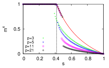
To determine whether the transition is first order or second order, we show the behavior of the magnetization $m^{x}$ in Fig. 2. The parameters of the figure correspond to those in Fig. 1. When $\lambda=0.1$, the magnetization $m^{x}$ for $p=3$ has a small jump at $s=0.3544(1)$, and $m^{x}$ for $p\geq 5$ decreases continuously from unity to our numerical precision. This means that $m^{z}$ for $p\geq 5$ increases continuously from zero to a finite value. Therefore a second-order transition occurs for $p\geq 5$ at $\lambda=0.1$. The same is true for $\lambda=0.3$ in the sense that there exists a second-order transition at the boundary of the QP2 phase for $p\geq 5$.

A remarkable fact is that the magnetization for some parameters (e.g., $\lambda=0.3$, $p=11$) in Fig. 2 jumps within the F phase. This discontinuity results in an exponential decrease of the energy gap as $N$ increases. There exists a first-order transition within the F phase. However, this unusual behavior disappears for smaller values of $\lambda$ for any finite $p$, excluding $p=3$, that we checked. Thus for smaller $\lambda$, only a second-order transition takes place as we increase $s$ from zero to a value close to unity.

The resulting phase diagrams are shown in Fig. 3 for $p=3,5$, and $11$. We see that a boundary of second-order transition exists for small $\lambda$ and $p\geq 5$. It is observed that one can reach the F phase from the QP phase by choosing a path that avoids a first-order transition as long as the first-order F-F boundary does not reach the $\lambda=0$ axis, which happens probably only in the limit $p\to\infty$ as we shall see below.

We next study the behavior of the energy gap across the phase transitions found in the previous section.

To calculate the energy gap for large $N$, we adopt the method used in [11]. The Hamiltonian under consideration is expressed by the components of total spin operator $\hat{S}^{x,z}$, thus commuting with the total spin $\hat{\bm{S}}$. Since the total angular momentum is conserved during the time evolution, we have to pay attention only to the subspace that has the maximum angular momentum $S=N/2$. The dimension of this subspace is $N+1$, which greatly enhances the possible system size to $N\sim 100$.

It is useful to first verify the validity of the static approximation. Figure 4 shows a representative energy gap with a second-order phase transition: As one sees in the enlarged view shown in the bottom panel, the gap shows wiggly behavior for a finite range. The wiggly behavior starts at $s\simeq 0.4184$ for $\lambda=0.3$, which corresponds to the left end of the QP2 domain and also to the second-order transition point between the QP and F phases. The same behavior terminates at $s\simeq 0.4676$ for $\lambda=0.3$, corresponding to the first-order F-F boundary. These two transition points evaluated analytically using the static approximation, Eqs. (18) and (19), are shown in dashed vertical lines in Fig. 4 and agree fairly satisfactorily with the numerical results, as $N$ increases, for the interval where the gap is very small.

The rightmost local minimum of the energy gap in Fig. 4 behaves differently from other local minima and decays exponentially as $N$ increases as shown in Fig. 5. This is expected from the jump in the magnetization shown in Fig. 2 because a jump implies a first-order transition though the system is ferromagnetic in both sides of the transition point. Although this is not the global minimum, it will affect the efficiency of QA for much larger systems where the rightmost one will become the global minimum since the other local minima decay only polynomially as shown below.

Figure 6 shows the size dependence of local minima of the energy gap for $p=5$ and $\lambda=0.1$. All minima shown here decay polynomially. In Fig. 7 the global minimum of energy gap for selected $p$ is depicted as a function of $N$ at $\lambda=0.1$. For any value of $p$, the gap closes polynomially at least up to the system size we studied, $N=160$.

The above results suggest that first-order transitions will be able to be avoided if we choose a path around $\lambda=0.1$ when we reach the F phase from the QP phase by increasing $s$ as long as $p$ is not too small and not too large, $5\leq p\leq 21$. It is then interesting to see what happens in the limit of large $p$.

References

- [1] M. R. Garey and D. S. Johnson, Computers and Intractability: A Guide to the Theory of NP-Completeness (Freeman, New York, 1979).
- [2] A. K. Hartmann and M. Weigt, Phase Transitions in Combinatorial Optimization Problems: Basics, Algorithms and Statistical Mechanics (Wiley-VCH, Weinheim, 2005).
- [3] J. J. Hopfield and D. W. Tank, Science 233, 625 (1986).
- [4] Y. Fu and P. W. Anderson, J. Phys. A 19, 1605 (1986).
- [5] T. Kadowaki and H. Nishimori, Phys. Rev. E 58, 5355 (1998).
- [6] A. B. Finnila, M. A. Gomez, C. Sebenik, C. Stenson, and J. D. Doll, Chem. Phys. Lett. 219, 343 (1994).
- [7] A. Das and B. K. Chakrabarti, Rev. Mod. Phys. 80, 1061 (2008).
- [8] E. Farhi, J. Goldstone, S. Gutmann, J. Lapan, A. Lundgren, and D. Preda, Science 292, 472 (2001).
- [9] S. Kirkpatrick, C. D. Gelatt, Jr., and M. P. Vecchi, Science 220, 671 (1983).
- [10] S. Morita and H. Nishimori, J. Math. Phys. 49, 125210 (2008).
- [11] T. Jörg, F. Krzakala, J. Kurchan, A. C. Maggs, and J. Pujos, EPL 89, 40004 (2010).
- [12] L. K. Grover, Phys. Rev. Lett. 79, 325 (1997).
- [13] T. Jörg, F. Krzakala, J. Kurchan, and A. C. Maggs, Phys. Rev. Lett. 101, 147204 (2008).
- [14] A. P. Young, S. Knysh, and V. N. Smelyanskiy, Phys. Rev. Lett. 104, 020502 (2010).
- [15] T. Jörg, F. Krzakala, G. Semerjian, and F. Zamponi, Phys. Rev. Lett. 104, 207206 (2010), arXiv:0911.3438v2.
- [16] E. Farhi, J. Goldstone, and S. Gutmann, arXiv:quant-ph/0208135.
- [17] M. Suzuki, Prog. Theor. Phys. 56, 1454 (1976).
- [18] H. Nishimori and G. Ortiz, Elements of Phase Transitions and Critical Phenomena (Oxford Univ. Press, Oxford, 2011).
- [19] There is no order parameter to characterize this phase transition in the sense the order parameter is finite in one phase and zero in the other. We nevertheless call it a phase transition because the energy (free energy) is singular at , . A similar phenomenon is observed within the ferromagnetic phase, a phase transition from a ferromagnetic phase to another ferromagnetic phase, as will be shown in Sec. IV.
- [20] R. Schützhold and G. Schaller, Phys. Rev. A 74, 060304 (2006).
- [21] It is to be noted that the special point has a highly degenerate ground state [24], among which only the state with the maximum total spin is relevant to our purpose: Quantum annealing starts from with and preserves the total spin following the Schrödinger equation (2) with .
- [22] E. Farhi, J. Goldstone, S. Gutmann, and M. Sipser, arXiv:quant-ph/0001106.
- [23] J. Roland and N. J. Cerf, Phys. Rev. A 65, 042308 (2002).
- [24] A. K. Chandra, J. Inoue, and B. K. Chakrabarti, Phys. Rev. E 81, 021101 (2010).