Minimum Cost Multicast with Decentralized SourcesThanks: N. Milosavljevic, S. Pawar, M. Gastpar and K. Ramchandran are with the Department of Electrical Engineering and Computer Science, University of California, Berkeley, Berkeley, CA 94720 USA (e-mail:{nebojsa,spawar, gastpar, kannanr}@eecs.berkeley.edu).Thanks: S. El Rouayheb is with the Department of Electrical Engineering, Princeton University, Princeton, NJ 08544 USA (e-mail: salim@princeton.edu).Thanks: M. Gastpar is also with the School of Computer and Communication Sciences, EPFL, Lausanne, Switzerland (e-mail: michael.gastpar@epfl.ch).Thanks: This research was funded by the NSF grants (CCF-0964018, CCF-0830788), a DTRA grant (HDTRA1-09-1-0032), and in part by an AFOSR grant (FA9550-09-1-0120).

We consider a multi-source multicast problem, over a given network topology with capacity constrained links. There are two types of nodes in the network; clients that are interested in recovering the whole content, and source nodes that may posses possibly correlated side-information. To further illustrate the problem set-up consider the following example.

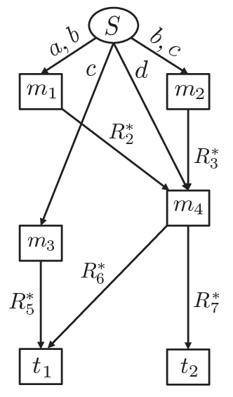
A file consists of four equally sized packets $a$, $b$, $c$ and $d$ belonging to some finite field $\mathbb{F}_{q^{n}}$. Also, suppose that the data packets are distributed across the nodes, $m_{1}$ through $m_{4}$, that are connected as shown in Figure 1. The clients denoted by $t_{1}$ and $t_{2}$ are interested in recovering the entire file. The edges in the graph are denoted by $e_{1},\ldots,e_{7}$ as shown in Figure 1. The objective is to minimize some function of the communication cost such that the clients $t_{1}$ and $t_{2}$ can recover the entire file. For instance, it can be shown that the following coding scheme minimizes the total number of bits communicated: node $m_{1}$ transmits $a$ on link $e_{2}$, node $m_{2}$ transmits $b,c$ on link $e_{3}$, node $m_{3}$ transmits $c$ on link $e_{5}$, node $m_{4}$ transmits $a,b,d$ on link $e_{6}$ and $a,b,c,d$ on link $e_{7}$.

Note that the example above considers a simple form of the side-information, where different nodes observe partial uncoded or “raw” data packets of the original file. Another important special case of side-information is when nodes observe linear combinations of the data packets of the original file. In a more general setting the side-information can be of more complex form i.e., arbitrary correlations.

The multisource multicast problem was originally studied by Ho, et al. [1], where for the linearly coded packets the authors showed under what conditions it is possible to recover the file at all destinations. For the case of uncoded packets, it is easy to show that one can add a super source as in [2] to the network and then using results from [3], find an optimal solution that minimizes the communication cost. In [4, 5] the authors considered a related problem over an undirected graph where all the nodes are interested in recovering the complete file. In [4] it was shown that the problem is NP-hard, while an approximate solution is provided in [5]. In [6], Haeupler et al. analyzed gossip based protocols in networks where each node observes correlated data.

In this paper, we make the following contributions.

• •

  In the case of most general scenario of arbitrarily correlated side information, we provide conditions as well as a polynomial time algorithm to determine when a multisource multicast problem over a given directed acyclic graph (DAG) is feasible.

• •

  Using submodular flow techniques, we provide a deterministic polynomial time algorithm to find number of bits each node should transmit in order to recover the file at all the clients and be optimal w.r.t. any linear cost function¹¹ 1 Linear cost function is defined w.r.t. the number of bits transmitted on each link..

• •

  For the special case of linearly correlated side information we provide an optimal communication scheme based on the algebraic network coding framework.

In this work we represent the network by a directed acyclic graph $G=(\mathcal{V},\mathcal{E})$, where $\mathcal{V}$ is the set of nodes, and $\mathcal{E}$ is the set of links that have capacity constraints. We define the capacity function $c:\mathcal{E}\rightarrow\mathbb{R}$ to denote the maximum number of bits that can be transmitted over a given link. We distinguish between two types of nodes: 1) source nodes $\mathcal{M}=\{m_{1},m_{2},\ldots,m_{l}\}$ that have partial information about the file, and 2) clients $\mathcal{T}=\{t_{1},t_{2},\ldots,t_{k}\}$ which are interested in recovering the file, and are sinks in the graph $G$. Let $X_{m_{1}},X_{m_{2}},\ldots,X_{m_{l}}$, denote the components of a discrete memoryless multiple source (DMMS) with a given joint probability mass function. Each source node $m_{i}\in\mathcal{M}$ observes $n$ i.i.d. realizations of the corresponding random variable $X_{m_{i}}$, denoted by $X_{m_{i}}^{n}$. We note that the results of this paper can be applied in a straightforward manner when the clients have side information as well. For the sake brevity, we focus on the case when clients have no side information.

The goal is for each client in $\mathcal{T}$ to gain access to all source nodes’ observations, i.e., to download the file. In order to achieve this goal, each node $m_{i}\in\mathcal{M}$ is allowed to send information across the graph $G$ at rate which is limited by the capacity of the outgoing links of that node. Transmission of each source node is a function of its own initial observation and all information it receives from its neighbors. Let us denote transmission on the link $e=(m_{i},m_{j})\in\mathcal{E}$ by

where $f_{e}(\cdot)$ is a mapping of the observations $X^{n}_{m_{i}}$ and transmissions received from the neighbors of $m_{i}$, $\{m_{r}:(m_{r},m_{i})\in\mathcal{E}\}$ to an outgoing message on the link $e$.

We denote by $\mathcal{M}_{t_{i}}\subseteq\mathcal{M}$ the set of source nodes which are connected to the client $t_{i}\in\mathcal{T}$. In other words, there exists a path in graph $G$ from every node in $\mathcal{M}_{t_{i}}$ to the client $t_{i}\in\mathcal{T}$. Consequently, we define the graph $G_{t_{i}}=(\mathcal{V}_{t_{i}},\mathcal{E}_{t_{i}})$ to be a subgraph of $G$, where $\mathcal{V}_{t_{i}}=\{\mathcal{M}_{t_{i}},t_{i}\}$, and $\mathcal{E}_{t_{i}}\subseteq\mathcal{E}$ is a set of links that connects all nodes in $\mathcal{M}_{t_{i}}$ among themselves and with client $t_{i}$. Furthermore, we assume that

where $X_{\mathcal{M}_{t_{i}}}\triangleq\left(X_{m_{j}}:m_{j}\in\mathcal{M}_{t_{i}}\right)$, and $X_{\mathcal{M}}\triangleq\left(X_{m_{1}},\ldots,X_{m_{l}}\right)$. Equality (2) ensures that every client in the network can potentially gain access to the entire process $X_{\mathcal{M}}$.

For each client $t_{i}\in\mathcal{T}$ to learn the file, transmissions $Fe$, $\forall e\in\mathcal{E}$, must satisfy,

In this work, we design a polynomial time algorithm for the multisource multicast problem that minimizes the linear cost function $\sum_{e\in\mathcal{E}}\alpha_{e}R_{e}$, where $\underline{\alpha}\triangleq(\alpha_{e}:e\in\mathcal{E}),~0<\alpha_{e}<\infty$, $\forall e\in\mathcal{E}$, is a vector of non-negative finite weights. We allow $\alpha_{e}$’s to be arbitrary non-negative constants, to account for the case when communication across some group of links in $G$ is more expensive compared to the others. Thus, the problem can be formulated as:

In order to solve the optimization problem in (5) we first establish a region called a “rate-flow region” that contains all possible optimal rate allocations. To identify this rate-flow region for our example of Figure 1, in the case of arbitrarily correlated side-information at the source nodes, we start by considering a single client $t_{1}$. Next, we isolate the subgraph $G_{t_{1}}=(\mathcal{V}_{t_{1}},\mathcal{E}_{t_{1}})$ corresponding to $t_{1}$ and modify its link capacities to infinity as shown in Figure 2.

Suppose the optimal solution w.r.t. problem (5) is achieved by $\mathbf{R}^{*}=(R^{*}_{1},\ldots,R^{*}_{6})$. Then, it follows that transmissions of node $m_{2}$ have to satisfy

Let us now consider node $m_{4}$. Its transmission includes information received from nodes $m_{1}$ and $m_{2}$ combined with its own side information. Since the goal is to minimize the total communication cost, it follows that for the optimal MM-rate vector $\mathbf{R}^{*}$, transmission of nodes $m_{1}$ and $m_{2}$ cannot be further compressed at node $m_{4}$. Therefore, the transmission of node $m_{4}$ consists of 2 components: 1) routed information from nodes $m_{1}$ and $m_{2}$, and 2)Innovative side-information at node $m_{4}$ w.r.t. all other source nodes in the network. Hence, $\mathbf{R}^{*}$ must satisfy

In order for client $t_{1}$ to recover the file, i.e., to gain access to $X_{\mathcal{M}_{t_{1}}}$, the incoming links to $t_{1}$ necessarily have to carry entire information about the process. In other words

where the equality sign comes from the fact that the goal is to minimize the overall communication cost, and thus, it is wasteful for client $t_{1}$ to receive at rate larger than the joint entropy of the process.

Considering all possible subsets of the source node set $\mathcal{M}_{t_{1}}$, we have that an optimal MM-rate vector $\mathbf{R}^{*}$ must belong to the following rate-flow region

where

and $\Delta^{+}\mathcal{S}\subseteq\mathcal{E}_{t_{1}},~(\Delta^{-}\mathcal{S}\subseteq\mathcal{E}_{t_{1}})$ denotes the set of links leaving (entering) $\mathcal{S}$. For instance, if $\mathcal{S}=\{m_{3},m_{4}\}$, then the optimal rate vector $\mathbf{R}^{*}$ satisfies

It can be verified that any rate vector that belongs to the rate-flow region $\partial\mathcal{R}_{t_{1}}$ can be achieved using multi-terminal Slepian-Wolf random-binning scheme [9]. Thus, the rate-flow region $\partial\mathcal{R}_{t_{1}}$ contains all optimal MM-rate vectors w.r.t. the optimization problem (5).

Extension of this result to a multiple client case is straightforward: an optimal MM-rate vector has to simultaneously belong to all rate-flow regions $\partial\mathcal{R}_{t_{i}}$ which correspond to the graph $G_{t_{i}}$, $\forall t_{i}\in\mathcal{T}$. Hence, the optimization problem (5) can be written as

Before we address the question of efficiently solving the problem (14), first we need to answer whether or not the problem is feasible.

As in Section III, first, we consider a single client case, i.e., when $\mathcal{T}=\{t_{1}\}$. Then, the obtained result naturally extends to the setting with arbitrary number of clients. Before we go any further, let us introduce some concepts from the combinatorial optimization theory which will turn out to be useful in proving our results. The set function $f:2^{\mathcal{M}_{t_{1}}}$ is supermodular if

If the inequality sign in (15) is reversed, then the function $f$ is called submodular. Let us define the polyhedron $P(f)$ and the base polyhedron $B(f)$ of a supermodular function $f$ as follows.

where $Z(\mathcal{S})=\sum_{i\in\mathcal{S}}Z_{i}$. Analogously, we define the polyhedron and the base polyhedron of a submodular function (the inequality signs in (16) and (17) are reversed).

It is easy to show that function

is supermodular. Hence, the rate-flow region $\partial\mathcal{R}_{t_{1}}$ defined in (11) represents the base polyhedron of the function $g_{t_{1}}$.

To verify whether there exists an achievable MM-rate vector it is necessary to check whether all $2^{|\mathcal{M}_{t_{1}}|}$ inequalities in (19) are satisfied. Verifying this is, in general, exponentially hard (in number of nodes). However, due to the supermodularity of the function $g_{t_{1}}$, the existence of a common base, and thus the feasibility of the multisource multicast problem, can be verified in polynomial time²² 2 Complexity of the common base algorithm proposed in [12] is $\mathcal{O}(|\mathcal{E}_{t_{1}}|^{3})$ (see [12] and [10], Chapter 4). This algorithm also provides an achievable MM-rate vector (given that it exists) that belongs to the rate-flow region $\partial\mathcal{R}_{t_{1}}$.

Extensions of the result of Lemma 1 to the case with arbitrary number of clients is straightforward. We just need to check if the inequalities (19) are satisfied for all clients in $\mathcal{T}$.

From [12], the common base problem, and hence the feasibility of the multisource multicast problem can be verified in $\mathcal{O}(k\cdot|\mathcal{E}|^{3})$ time.

In this section we propose a polynomial time deterministic algorithm that solves optimization problem (14). As in Section IV, we begin by considering a single client case, i.e., when $\mathcal{T}=\{t_{1}\}$. Then, by using a similar methodology as in [3], we extend our solution to the arbitrary number of clients.

In this work we study the linear cost multisource multicast problem, where each node in the network observes i.i.d. copies of the DMMS process. Assuming that nodes can communicate over the capacity constrained links of the directed acyclic graph, the goal is for each client (sink of the graph), to learn the file, while minimizing a linear communication cost. First, we show that the underlying optimization problem can be posed as a linear program with exponentially many rate-flow constraints. Then, we provide the “capacity flow” conditions under which the multisource multicast problem is feasible. Applying the common base algorithm one can construct a test that verifies feasibility in polynomial time. We show that the linear cost multisource multicast problem with single client and many nodes can be solved in polynomial time by applying algorithms for the minimum cost submodular flow problem. Further, using the single client solution as a building block we show how one can solve a more general problem with arbitrary number of clients in polynomial time. For the special case of the finite linear source model, we propose a polynomial time algorithm that computes an explicit transmission scheme.

References

- [1] T. Ho, R. Koetter, M. Médard, M. Effros, J. Shi, and D. Karger, “A random linear network coding approach to multicast,” IEEE Transactions on Information Theory, vol. 52, no. 10, pp. 4413–4430, October 2006.
- [2] S. Tajbakhsh, P. Sadeghi, and R. Shams, “A generalized model for cost and fairness analysis in coded cooperative data exchange,” in Network Coding (NetCod), 2011 International Symposium on. IEEE, 2011, pp. 1–6.
- [3] D. Lun, N. Ratnakar, M. Médard, R. Koetter, D. Karger, T. Ho, E. Ahmed, and F. Zhao, “Minimum-cost multicast over coded packet networks,” Information Theory, IEEE Transactions on, vol. 52, no. 6, pp. 2608–2623, 2006.
- [4] T. Courtade, B. Xie, and R. Wesel, “Optimal Exchange of Packets for Universal Recovery in Broadcast Networks,” in Proceedings of Military Communications Conference, 2010.
- [5] M. Gonen and M. Langberg, “Coded cooperative data exchange problem for general topologies,” Arxiv preprint arXiv:1202.2088, 2012.
- [6] B. Haeupler, A. Cohen, C. Avin, and M. Médard, “Network coded gossip with correlated data,” Arxiv preprint arXiv:1202.1801, 2012.
- [7] C. Chan, “Generating Secret in a Network,” Ph.D. dissertation, Massachusetts Institute of Technology, 2010.
- [8] R. Koetter and M. Medard, “An Algebraic Approach to Network Coding,” IEEE/ACM Transactions on Networking, vol. 11, no. 5, pp. 782 – 795, 2003.
- [9] T. Cover and J. Thomas, “Elements of information theory 2nd edition,” 2006.
- [10] S. Fujishige, Submodular functions and optimization. Elsevier Science, 2005.
- [11] A. Hoffman, “Some recent applications of the theory of linear inequalities to extremal combinatorial analysis,” New York, NY, pp. 113–117, 1958.
- [12] E. Lawler and C. Martel, “Computing maximal polymatroidal network flows,” Mathematics of Operations Research, vol. 7, no. 3, pp. 334–347, 1982.
- [13] S. Fujishige and S. Iwata, “Algorithms for submodular flows,” IEICE Transactions on Information and Systems, vol. 83, pp. 322–329, 2000.
- [14] H. Sherali and G. Choi, “Recovery of primal solutions when using subgradient optimization methods to solve lagrangian duals of linear programs,” Operations Research Letters, vol. 19, no. 3, pp. 105–113, 1996.
- [15] N. Harvey, D. Karger, and K. Murota, “Deterministic network coding by matrix completion,” in Proceedings of the sixteenth annual ACM-SIAM symposium on Discrete algorithms, 2005, pp. 489–498.