Substructure and Boundary Modeling for Continuous Action Recognition
Abstract
This paper introduces a probabilistic graphical model for continuous action recognition with two novel components: substructure transition model and discriminative boundary model. The first component encodes the sparse and global temporal transition prior between action primitives in state-space model to handle the large spatial-temporal variations within an action class. The second component enforces the action duration constraint in a discriminative way to locate the transition boundaries between actions more accurately. The two components are integrated into a unified graphical structure to enable effective training and inference. Our comprehensive experimental results on both public and in-house datasets show that, with the capability to incorporate additional information that had not been explicitly or efficiently modeled by previous methods, our proposed algorithm achieved significantly improved performance for continuous action recognition.
1 Introduction
Understanding continuous human activities from videos, i.e. simultaneous segmentation and classification of actions, is a fundamental yet challenging problem in computer vision. Many existing works approach the problem using bottom-up methods [32], where segmentation is performed as preprocessing to partition videos into coherent constituent parts, and action recognition is then applied as an isolated classification step. Although a rich literature exists for segmentation of time series, such as change point detection [12], periodicity of cyclic events modeling [7] and frame clustering [40], the methods tend to detect local boundaries and lack the ability to incorporate global dynamics of temporal events, which leads to under or over segmentation that severely affects the recognition performance, especially for complex actions with diversified local motion statistics [13].


The limitation of the bottom-up approaches has been addressed by performing concurrent top-down recognition using variants of Dynamic Bayesian Network (DBN), where the dynamics of temporal events are modeled as transitions in a latent [25, 18] or partially observed state space [14, 28]. The technique has been successfully used in speech recognition and natural language processing, while the performance of existing DBN based approaches for action recognition [28, 10, 33, 34, 17, 27] tends to be relatively lower [13], mostly due to the difficulty in interpreting the physical meaning of latent states. Thus, it becomes difficult to impose additional prior knowledge with clear physical meaning into an existing graphical structure to further improve its performance.
To tackle the problem, in this paper, we show how two additional sources of information with clear physical interpretations can be considered in a general graphical structure for state-space model (SSM) in Figure 1. Compared to a standard Switching Linear Dynamic System (SLDS) [28] model in Figure 1.(a), where , and are respectively the hidden state, observation and label, the proposed model in Figure 1.(b) is augmented with two additional nodes, and , to describe the substructure transition and duration statistics of actions:
Substructure transition Rather than a uniform motion type, a real-world human action is usually characterized by a set of inhomogeneous units with some instinct structure, which we call substructure. Action substructure arises from two factors: (1) the hierarchical nature of human activity, where one action can be temporally decomposed into a series of primitives with spatial-temporal constraints; (2) the large variance of action dynamics due to differences in kinematical property of subjects, feedback from environment, or interaction with objects. For the first factor, Hoai et al. [13] used multi-class Support Vector Machine (SVM) with Dynamic Programming to recognize coherent motion constituent parts in an action; Liu et al. [23] applied latent-SVM for temporal evolving of “attributes” in actions; Sung et al. [34] introduced a two-layer Maximum Entropy Markov Models to recognize the correspondence between sub-activities and human skeletal features. For the second factor, considerations have been paid to the substructure variance caused by subject-object interaction using Connected Hierarchic Conditional Random Field (CRF) [17], and the substructure variance caused by pose using Latent Pose CRF [27].
In more general cases, Morency et al. presented the Latent Dynamic CRF (LDCRF) algorithm by adding a “latent-dynamic” layer into CRF for hidden substructure transition [26]. The limitation of CRF as a discriminative method is that, one single pseudo-likelihood score is estimated for an entire sequence which is incapable to interpret the probability of each individual frame. To solve the problem, we instead design a generative model as in Figure.1.(b), with extra hidden node gating the transition amongst a set of dynamic systems, and the posterior for every action can be inferred strictly under Bayesian framework for each frame. The dimension of state space increases geometrically with an extra hidden node, so we introduce effective transition prior constraints in Section 2 to avoid over-fitting on a limited amount of training data.
Duration model The duration statistics of actions is important in determining the boundary where one action transits to another in continuous recognition tasks. Duration model has been widely adopted in Hidden Markov Model (HMM) based methods, such as the explicit duration HMM [9] or more generally the Hidden Semi Markov Model (HSMM) [39]. Incorporating duration model into SSM is more challenging than HMM because SSM has continuous state space, and exact inference in SSM is usually intractable [20]. Some works reported in this line include Cemgil et al. [5] for music transcription and Chib and Dueker [6] for economics. Oh et al. [29] imposed the duration constraint at the top level of SLDS and achieved improved performance for honeybee behavior analysis [28]. In general, naive integration of duration model into SSM is not effective, because duration patterns vary significantly across visual data and limited training samples may bias the model with incorrect duration patterns.
To address this problem, in Figure 1.(b) we correlate duration node with the continuous hidden state node and the substructure transition node via logistic regression as explained in Section 3. In this way, the proposed duration model becomes more discriminative than conventional generative models, and the data-driven boundary locating process can accommodate more variation in duration length.
In summary, the major contribution of the paper is to incorporate two additional models into a general SSM, namely the Substructure Transition Model (STM) and the Discriminative Boundary Model (DBM). We also design a Rao-Blackwellised particle filter for efficient inference of proposed model in Section 4. Experiments in Section 5 demonstrate the superior performance of our proposed system over several existing state-of-the-arts in continuous action recognition. Conclusion is drawn in Section 6.
2 Substructure Transition Model
Linear Dynamic Systems (LDS) is the most commonly used SSM to describe visual features of human motions. LDS is modeled by linear Gaussian distributions:
| (1) |
| (2) |
where is the observation at time , is a latent state, is multivariate normal distribution of with mean and covariance . To consider multiple actions, SLDS [28] is formulated as a mixture of LDS’s with the switching among them controlled by action class . However, each LDS can only model an action with homogenous motion, ignoring the complex substructure within the action. We introduce a discrete hidden variable to explicitly represent such information, and the substructured SSM can be stated as:
| (3) |
| (4) |
where , , , and are the LDS parameters for the action primitive in the substructure of action class. is modeled as a Markov chain and the transition probability is specified by multinomial distribution:
| (5) |
In the following, the term STM may refer to either the transition matrix in Eq. (5) or the overall substructured SSM depending on its context. Some examples of STM are given in Fig. 2, which are to be explained in detail in the remainder of this section.


2.1 Sparsity Constrained STM
We use simplified notation for the STM within a single action. In general, can be any matrix as long as each row of it is a probability vector, which allows the substructure of action primitives to be organized arbitrarily. For most real-world human actions, however, there is a strong temporal ordering associated with the primitive units. Such order relationship can be vital to accurate action recognition, since a different temporal ordering can define a totally different action even if the composing primitive units are the same. Moreover, if prior information of substructure is incorporated in model estimation, the learning process can become more robust to noise and outliers.
There have been some attempts to characterize the order relationship of primitive units by restricting the structure of transition matrix . For example, left-to-right HMM [2] is proposed to model sequential or cyclic ordering of primitive units, and the corresponding has non-zero values only on or directly above diagonal, as illustrated in Fig. 2 (a). Sequential ordering is a very strong assumption; to describe actions with more flexible temporal patterns, people have resorted to switching HMM [14] or factorial HMM [11], which model action variations with multiple sequential orderings. All the works above assume the order relationship between action units are given a priori; i.e. , the number of non-zero entries in is small and their locations are all known. In many cases, however, it is difficult to specify such information exactly, and making a wrong assumption can bias the estimation of action model. A more practical approach is to impose a sparse transition constraint while leaving the discovery of exact order relationship to training phase. Along this direction, negative Dirichlet distribution has been proposed in [4] as a prior for each row in :
| (6) |
where is a pseudo count penalty. The MAP estimation of parameter is
| (7) |
where is the sufficient statistics of . When the number of transitions from to in training data is less than , the probability is set to zero. The sparsity enforced in this way often leads to local transition patterns which might be actually caused by noise or incomplete data, as shown in Fig. 2 (b). Also, the penalty term introduces bias to the proportion of non-zero transition probabilities, i.e. . This bias can be severe especially when is small.
2.2 Block-wise Sparse STM
As we have seen, the sequential order assumption about the transition between action units is too strong, while the sparse prior on transition probability is biased and cannot globally regularize the STM. Here we propose a block-wise sparse STM which can achieve tradeoff between model sparsity and flexibility. The idea is to divide an action into several stages and each stage comprises of a subset of action primitives. The transition between stages is encouraged to be sequential but sparse, such that the global action structure can be modeled. At the same time, the action primitives within each stage can propagate freely from one to another so that variation in action styles and parameters is also preserved. Our stage-wise transition model is also favorable in regard of continuous action segmentation, since the starting and terminating stages can be explicitly modeled to enhance discrimination on action boundaries.
Formally, define discrete variable as the current stage index of action, and assume a surjective mapping is given which assigns each action primitive to its corresponding stage :
| (8) |
The choice of depends on the nature of action. Intuitively, we can assign more action primitives to a stage with diversified motion patterns and less action primitives to a stage with restricted pattern. The joint dynamic transition distribution of and is defined as:
| (9) |
The second term of Eq. (9) specifies the transition between action primitives, which we want to keep as flexible as possible to model diversified local action patterns. The first term captures the global structure between different action stages, and therefore we impose an ordered negative Dirichlet distribution as its hyper-prior:
| (10) |
where is the stage transition probability matrix, , and is a constant for pseudo count penalty. The ordered negative Dirichlet prior encodes both sequential order information and sparsity constraint. It promotes statistically a global transition path which can be learned from training data rather than heuristically defined as in left-to-right HMM [2]. An example of the resulting STM is shown in Fig. 2 (c). Note that no in-coming/out-going transition is encouraged for /, which stands for starting/terminating stage. The identification of these two special stages is helpful for segmenting continuous actions, as will be discussed in Sec. 3.2.
2.3 Learning STM
The MAP model estimation requires maximizing the product of likelihood (9) and prior (10) under the constraint of (8). There are two interdependent nodes, and , involved in the optimization, which make the problem complicated. Fortunately, as shown in Appendix A, Eq. (9) can be replaced with the transition distribution of single variable and a constraint exists for the relationship between and . Therefore, the node (and the associated parameter ) serves only for conceptual purpose and can be eliminated in our model construction. The MAP estimation can be converted to the following constrained optimization problem:
| (11) | |||||
where is the sufficient statistics of , , and are just auxiliary variables. The KKT (Karush-Kuhn-Tucker) conditions for optimal solution are:
where , , and are constant multipliers; is equal to if or , and otherwise. Solving the equation set as in Appendix B gives the MAP parameter estimation:
| (12) | |||||
As we can see, the resultant transition matrix is a block-wise sparse matrix, which can characterize both the global structure and local detail of action dynamics. Also, within each block (stage), there is no bias in .
3 Discriminative Boundary Model
3.1 Logistic Duration Model
It is straightforward to use a Markov chain to model the transition of action where . The duration information of the action is naively incorporated into its self-transition probability , which leads to an action duration model with exponential distribution:
Unfortunately, only a limited number of real-life events have an exponentially diminishing duration. Inaccurate duration modeling can severely affect our ability to segment consecutive actions and identify their boundaries.
Non-exponential duration distribution can be implemented with duration-dependent transition matrix, such as the one used in HSMM [39]. Fitting a transition matrix for each epoch within the maximum length of duration is often impossible given a limited number of training sequences, even when parameter hyperprior such as hierarchical Dirichlet distribution [36] is used to restrict model freedom. Parametric duration distributions such as gamma [21] and Gaussian [38] provide a more compact way to represent duration and show good performance in signal synthesis. However, they are less useful in inference because the corresponding transition probability is not easy to evaluate.
Here a new logistic duration model is proposed to address the above limitations. We introduce a variable to represent the length of time current action has been lasting. is a counting process starting from , and the beginning of a new action is triggered whenever it is reset to :
| (13) |
where is the probability of transiting from previous action to new action . Notice that the same type of action can be repeated if we have .
Instead of modeling action duration distribution directly, we model the transition distribution of as a logistic function of its previous value:
| (14) |
| (15) |
where and are positive logistic regression weights. Eq. (14) immediately leads to the duration distribution for action class :
| (16) |
Fig. 3 (a) shows how the resetting probability of changes as a function of with different parameter sets, and the corresponding duration distributions are plotted in (b). The increasing probability of transiting to a new action leads to a peaked duration distribution, with center and width controlled by and , respectively. Our logistic duration model can be easily extended to represent multiple-mode durations if double logistic function [22] is used.


3.2 Discriminative Boundary Model
The logistic duration model can be integrated with STM by stacking the two layers of nodes (- and --) together. The resultant generative model, however, is unable to utilize contextual information for accurate action boundary segmentation. Discriminative graphic models, such as MEMM [25] and CRF [18], are generally more powerful in such classification problem except that they ignore data likelihood or suffer from label bias problem.
To integrate discriminating power into our action boundary model and at the same time keep the generative nature of the action model itself, we construct DBM by further augmenting the duration distribution (which triggers action boundary) with the contextual information from latent states and :
| (17) |
where , have the same meaning as in Eq. (14), and are the additional logistic regression coefficients. When , no information can be learned from and , and the DBM reduces to a generative one as Eq. (14). A similar logistic function has been employed in augmented SLDS [3], where the main motivation is to distinguish between transitions to different states based on latent variable. Our DBM is specifically designed for locating the boundary between contiguous actions. It relies on both real valued and categorical inputs.
As constrained by the STM in Subsection 2.2, each action is only likely to terminate in stage . Therefore, can be reset to only when the current action in this terminating stage, and we can modify Eq. (17) as:
| (18) |
In this way, the number of parameters is greatly reduced and the label unbalance problem is also ameliorated. Now, the construction of our action model for continuous recognition has been completed, with the overall structure shown in Figure 1 (b).
3.3 Learning DBM
To learn the parameters , and , we use coordinate descent method to iterate between and . For and , given a set of training sequences with class labels , we can easily obtain the values for all duration nodes according to Eq. (13)-(15). Then fitting the parameters and is equivalent to performing logistic regression with input-output pairs . The action transition probability can be obtained trivially.
To estimate , let be our training set, where each data sample is a realization of all the nodes involved in Eq. (17) at a particular time instance and . Since and are hidden variables, their posterior and are first inferred from single action STM, where the posterior of is approximated by a Gaussian. The estimation of is obtained by maximizing the expected log likelihood:
| (19) | ||||
where
| (20) |
and , . The integral in Eq. (19) cannot be solved analytically. Instead, we use unscented transform [15] to approximate the integral with the average over a set of sigma points of :
where is the dimension of , is the column of the matrix square root of . Therefore, Eq. (19) converts to a weighted logistic regression problem with features , labels and weights .
4 Inference with Rao-Blackwellised Particle Filter
In testing, given an observation sequence , we want to find the MAP action labels and the boundaries defined by ; we are also interested in the style of actions which can be revealed from . To obtain these MAP estimates, we are required to find the posterior , which is a non-trivial job given the complicated hierarchy and nonlinearity of our model. We propose to use particle filtering [1] for online inference due to its capability in non-linear scenario. Moreover, the latent variable can be marginalized by Rao-Blackwellisation [8]. In this way, the computation of particle filtering is significantly reduced since Monte Carlo sampling is only conducted in the joint space of , which has a much lower dimension and a highly compact support (note the sparse transition probability between these variables).
Formally, we decompose the posterior distribution of all the hidden nodes at time as
| (21) |
where the second term can be evaluated analytically because depends on other variables through linear and Gaussian relations. In Rao-Blackwellised particle filter [16], a set of samples and the associated weights are used to approximate the intractable first term, while the second term is represented by , which are analytical distributions of conditioned on corresponding samples:
| (22) |
In our model, is a Gaussian distribution. Thus, the posterior can be represented as
| (23) |
where the approximation error approaches to zero as increases to infinite.
Given the samples and weights at time , the posterior of at time is:
where
| (24) |
The detailed derivation is shown in Appendix C. It is hard to draw sample from Eq. (24). Instead, we draw new samples from a proposal density defined as:
| (25) |
The new sample weights are then updated as follows:
| (26) |
is essentially the integral of a Gaussian function with a logistic function. Although not solvable analytically, it can be well approximated by a re-parameterized logistic function according to [24]. Details on how to evaluate can be found in Appendix D.
Once we get and , is simply updated by Kalman filter. Re-sampling and normalization procedures are applied after all the samples are updated as in [8].
5 Experimental Results
Our model is tested on four datasets for continuous action recognition. In all the experiments, we have used parameters , , . First STM is trained independently for each action using the segmented sequences in training set; then DBM is learned from the inferred terminal stage of each sequence. The overall learning procedure follows EM paradigm where the beginning and terminating stages are initially set as the first and last of each sequence, and the initial action primitives are obtained from K-means clustering. In testing, after the online inference using particle filter, we further adjust each action boundary using an off-line inference within a local neighborhood of length centered at the initial boundary; in this way, the locally “full” posterior in Sec. 4 is considered. We evaluate the recognition performance by per-frame accuracy. Contribution from each model component (STM and DBM) is analyzed separately.
5.1 Public Dataset
The first public dataset used is the IXMAS dataset [37]. The dataset contains 11 actions, each performed 3 times by 10 actors. The videos are acquired using 5 synchronized cameras from different angles, and the actors freely changed their orientation in acquisition. We calculate dense optical flow in the silhouette area of each subject, from which Locality-constrained Linear Coding features (LLC)11 1 implementation from author’s website [35] are extracted as the observation in each frame. We have used 32 codewords and , and spatial pyramid [19]. Table 1 reports the continuous action recognition results, in comparison with SLDS22 2 implementation based on BNT from http://code.google.com/p/bnt/ [28], CRF11footnotemark: 1 [18] and LDCRF11footnotemark: 1 [26]. Our proposed model (and each of its components) achieves a recognition accuracy higher than all the other methods by more than .
| SLDS | CRF | LDCRF | STM | DBM | STM+DBM |
|---|---|---|---|---|---|
| 53.6% | 60.6% | 57.8% | 70.2% | 74.5% | 76.5% |
The second public dataset used is the CMU MoCap dataset 33 3 http://mocap.cs.cmu.edu/. For comparison purpose, we report the results from the complete subset of subject 86. The subset has 14 sequences with 122 actions in 8 category. Quaternion feature is derived from the raw MoCap data as our observation for inference. Table 2 lists the continuous action recognition results, in comparison with the same set of benchmark techniques as in the first experiment, as well as [30, 31]. Similarly, results from this experiment demonstrated the superior performance of our method. It is interesting to note that, in Table 2, the frame-level accuracy by using DBM alone is a little higher than its combination with STM. This is because there’s only one subject in this experiment and no significant variation in substructure is presented in each action type, so temporal duration plays a more important role in recognition. Nevertheless, the result attained by STM+DBM is superior than all benchmark methods.
5.2 In-house dataset
| SLDS | CRF | LDCRF | [30] | [31] | STM | DBM | STM+DBM |
|---|---|---|---|---|---|---|---|
| 80.0% | 77.2% | 82.5% | 72.3% | 90.9% | 81.0% | 93.3% | 92.1% |
In addition to the above two public datasets, two in-house datasets were also captured. The actions in these two sets feature stronger hierarchical substructure. The first dataset contains videos of stacking/unstacking three colored boxes, which involves actions of ‘‘move-arm’’, ‘‘pick-up’’ and ‘‘put-down’’. 13 sequences with 567 actions were recorded in both RGB and depth videos with one Microsoft Kinect sensor 44 4 http://www.xbox.com/kinect (Fig. 4). Then object tracking and 3-D reconstruction were performed to obtain the 3D trajectories of two hands and three boxes. In this way an observation sequence in is generated. In the experiments, leave-one-out cross-validation was performed on the 13 sequences. The continuous recognition results are listed in Table 3. It is noticed that, among the four benchmark techniques, the performance of SLDS and CRF are comparable, while LDCRF achieved the best performance. This is reasonable because during the stacking process, each box can be moved/stacked at any place on the desk, which leads to large spatial variations that cannot be well modeled by a Bayesian Network of only two layers. LDCRF applied a third layer to capture such “latent dynamics”, and hence achieved best accuracy. For our proposed models, the STM alone brings LDS to a comparable accuracy to LDCRF because it also models the substructure transition pattern. By further incorporating duration information, our model outperforms all other existing approaches.
The second in-house dataset is more complicated than the first one. It involves five actions, “move-arm”, “pick-up”, “put-down”, “plug-in” and “plug-out”, in a printer part assembling task (Fig. 5). The 3D trajectories of two hands and two printer parts were extracted using the same Kinect sensor system. 8 sequences were recorded and tested with leave-one-out cross-validation. As can be seen from Table 4, our proposed model with both STM and DBM outperforms other benchmark approaches by a large margin.
 |
| (a) Set I: Stacking |
 |
| (b) Set II: Assembling |
| SLDS | CRF | LDCRF | STM | DBM | STM+DBM |
|---|---|---|---|---|---|
| 64.4% | 79.6% | 90.3% | 88.5% | 81.3% | 94.4% |
| SLDS | CRF | LDCRF | STM | DBM | STM+DBM |
|---|---|---|---|---|---|
| 68.2% | 77.7% | 88.5% | 88.7% | 69.0% | 92.9% |
5.3 Discussion
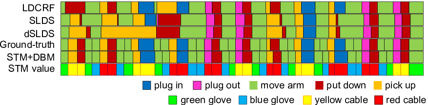
To provide more insightful comparison between the proposed algorithm and other benchmark algorithms, we show two examples of continuous action recognition results from the in-house datasets in Fig. 6. The result given by SLDS contains short and frequent switchings between incorrect action types. This is caused by the false matching of motion patterns to an incorrect action model. dSLDS [29] and LDCRF eliminate the short transitions by considering additional context information; however, their performances degrade severely around noisy or ambiguous action periods (e.g. the beginning of the sequence in Fig. 6.(b)) due to false duration prior or overdependence on discriminative classifier. Our proposed STM+DBM approach does not suffer from any of these problems, because STM helps to identify all action classes disregarding their variations, and DBM further helps to improve the precision of boundaries with both generative and discriminative duration knowledge. Another interesting finding shown in the last rows of (a) and (b) is that the substructure node can be interpreted by concrete physical meanings. For all the actions in these experiments, we find different object involved in an action corresponds to a different value of , which dominates the infer values in that action. Therefore, in addition to estimating action class, we can also find the object associated with the action by majority voting based on . In our experiments, all the inferred object associations agree with ground truth.
6 Conclusion and Future Work
In this paper, we introduce an improved SSM with two added layers modeling the substructure transition dynamics and duration distribution for human action. The first layer encodes the sparse and global temporal transition structure of action primitives and also maintains action variations. The second layer injects discriminative information into a logistic duration model and discovers action boundaries more adaptively. We design a Rao-Blackwellised particle filter for efficient inference. Our comprehensive experimental results validate the effectiveness of both two layers of our model in continuous action recognition. As future work we plan to apply our model to actions in less constrained scenarios and use more advanced low-level descriptors to deal with unreliable observations.
Appendix A Derivation of Eq.(11)
Appendix B Derivation of Eq.(12)
Appendix C Derivation of Eq.(4) and (24)
Appendix D Evaluation of Eq.(24)
The above two Gaussian distributions, i.e. the first two terms in the integral of Eq.(24), can be combined as a single Gaussian of . Omit all the subscriptions, and the product of exponential terms is:
where
Therefore, the product of two Gaussian is:
where
The third term in the integral of Eq.(24), defined in Eq.(17), can be re-written as:
where , , and is logistic (or Fermi) function. The probability for can be obtained accordingly.
To convert the integral in Eq.(24) into a single variable integral, we further introduce a linear transformation:
where is orthonormal, and . For Gaussian variable, we have:
Therefore,
References
- [1] M. Arulampalam, S. Maskell, N. Gordon, and T. Clapp. A tutorial on particle filters for on-line nonlinear/non-Gaussian Bayesian tracking. IEEE Trans. on Signal Processing, 50(2):174–188, 2002.
- [2] R. Bakis. Continuous speech word recognition via centisecond acoustic states. unpublished paper presented at the meeting of the Acoustics Society of America, 1976.
- [3] D. Barber. Expectation correction for smoothed inference in switching linear dynamical systems. Journal of Machine Learning Research, pages 2515–2540, 2006.
- [4] M. Bicego, M. Cristani, and V. Murino. Sparseness achievement in hidden Markov models. Proc.of ICIAP’07, pages 67–72, 2007.
- [5] A. Cemgil, H. Kappen, and D. Barber. A generative model for music transcription. In IEEE Transactions on Audio, Speech, and Language Processing, pages 679–694, 2006.
- [6] S. Chib and M. J. Dueker. Non-Markovian regime switching with endogenous states and time-varying state strengths. Econometric Society 2004 North American Summer Meetings 600, Econometric Society, 2004.
- [7] R. Cutler and L. Davis. Robust real-time periodic motion detection, analysis, and applications. IEEE Trans. on Pattern Analysis and Machine Intelligence, 22(8):781–796, 2000.
- [8] A. Doucet, N. d. Freitas, K. P. Murphy, and S. J. Russell. Rao-Blackwellised particle filtering for dynamic Bayesian networks. In Proceedings of the 16th Conference on Uncertainty in Artificial Intelligence, pages 176–183, 2000.
- [9] J. Ferguson. Variable duration models for speech. Symp. Application of Hidden Markov Models to Text and Speech, Institute for Defense Analyses, Princeton, NJ, pages 143–179, 1980.
- [10] E. Fox, E. Sudderth, M. Jordan, and A. Willsky. Nonparametric Bayesian learning of switching linear dynamical systems. Proc. of NIPS’09, 2009.
- [11] Z. Ghahramani and M. Jordan. Factorial hidden Markov models. Proc.of NIPS, 1996.
- [12] Z. Harchaoui, F. Bach, and E. Moulines. Kernel changepoint analysis. Proc. of NIPS’09, 2009.
- [13] M. Hoai, Z. Lan, and F. Torre. Joint segmentation and classification of human action in video. Proc. of CVPR’11, 2011.
- [14] M. Hoffken, D. Oberhoff, and M. Kolesnik. Switching hidden Markov models for learning of motion patterns in videos. Proc. of ICANN’09, pages 757–766, 2009.
- [15] S. Julier and J. Uhlmann. A new extension of the Kalman filter to nonlinear systems. Proc of AeroSense: The 11th International Symposium on Aerospace/Defence Sensing, Simulation and Control, pages 182–193, 1997.
- [16] Z. Khan, T. Balch, and F. Dellaert. A Rao-Blackwellized particle filter for EigenTracking. In Proceedings of the IEEE computer society conference on Computer vision and pattern recognition, pages 980–987, 2004.
- [17] H. Kjellstrom, J. Romero, D. Martinez, and D. Kragic. Simultaneous visual recognition of manipulation actions and manipulated objects. Proc. of ECCV’08, 2008.
- [18] J. Lafferty, A. McCallum, and F. Pereira. Conditional random fields: probabilistic models for segmenting and labeling sequence data. Proc. of ICML’01, 2001.
- [19] S. Lazebnik, C. Schmid, and J. Ponce. Beyond bags of features: spatial pyramid matching for recognizing natural scene categories. Proc. of CVPR’06, 2006.
- [20] U. Lerner and R. Parr. Inference in hybrid networks: theoretical limits and practical algorithms. In In UAI, pages 310–318, 2001.
- [21] S. Levinson. Continuously variable duration hidden Markov models for automatic speech recognition. Comput. Speech Lang., pages 29–45, 1986.
- [22] S. Lipovetsky. Double logistic curve in regression modeling. Journal of Applied Statistics, pages 1785–793, 2010.
- [23] J. Liu, B. Kuipers, and S. Savarese. Recognizing human actions by attributes. Proc. of CVPR’11, 2011.
- [24] P. Maragakis, F. Ritort, C. Bustamante, M. Karplus, and G. E. Crooks. Bayesian estimates of free energies from nonequilibrium work data in the presence of instrument noise. Journal of Chemical Physics, 129, 2008.
- [25] A. McCallum, D. Freitag, and F. Pereira. Maximum entropy Markov models for information extraction and segmentation. Proc. of ICML’00, pages 591–598, 2000.
- [26] L. Morency, A. Quattoni, and T. Darrell. Latent-dynamic discriminative models for continuous gesture recognition. Proc. of CVPR’07, 2007.
- [27] H. Ning, W. Xu, Y. Gong, and T. Huan. Latent pose estimator for continuous action recognition. Proc. of ECCV’08, 2008.
- [28] S. Oh, J. Rehg, T. Balch, and F. Dellaert. Learning and inference in parametric switching linear dynamic systems. Proc. of ICCV’05, 2005.
- [29] S. M. Oh, J. M. Rehg, and F. Dellaert. Parameterized duration modeling for switching linear dynamic systems. Proc. of CVPR’06, pages 1–8, 2006.
- [30] N. Ozay, M. Sznaier, and C. O. Sequential sparsificarion for change detection. Proc. of CVPR’08, 2008.
- [31] M. Raptis, K. Wnuk, and S. Soatto. Spike train driven dynamical models for human actions. Proc. of CVPR’10, pages 2077–2084, 2010.
- [32] S. Satkin and M. Hebert. Modeling the temporal extent of actions. Proc. of ECCV’10, 2010.
- [33] C. Sminchisescu, A. Kanaujia, Z. Li, and D. Metaxas. Conditional models for contextual human motion recognition. Proc. of ICCV’05, 2005.
- [34] J. Sung, C. Ponce, B. Selman, and A. Saxena. Human activity detection from RGBD images. Proc. of AAAI’11, 2011.
- [35] J. Wang, J. Yang, F. Lv, and K. Yu. Locality-constrained linear coding for image classification. Proc. of CVPR’10, 2010.
- [36] Z. Wang, E. Kuruoglu, X. Yang, Y. Xu, and S. Yu. Event recognition with time varying hidden Markov model. Proc.of ICASSP’09, pages 1761–1764, 2009.
- [37] D. Weinland, R. Ronfard, and E. Boyer. Free viewpoint action recognition using motion history volumes. Computer Vision and Image Understanding, 2006.
- [38] T. Yoshimura, K. Tokuda, T. Masuko, T. Kobayashi, and T. Kitamura. Duration modeling for HMM-based speech synthesis. Proc. of ICSLP’98, 1998.
- [39] S.-Z. Yu. Hidden semi-Markov models. Artificial Intelligence, pages 215–243, 2010.
- [40] F. Zhou, F. Torre, and J. K. Hodgins. Aligned cluster analysis for temporal segmentation of human motion. Proc. of IEEE Conference on Automatic Face and Gestures Recognition, 2008.