Stability of freely falling granular streams
Abstract
A freely falling stream of weakly cohesive granular particles is modeled and analysed with help of event driven simulations and continuum hydrodynamics. The former show a breakup of the stream into droplets, whose size is measured as a function of cohesive energy. Extensional flow is an exact solution of the one-dimensional Navier- Stokes equation, corresponding to a strain rate, decaying like from its initial value, . Expanding around this basic state, we show that the flow is stable for short times, , whereas for long times, , perturbations of all wavelength grow. The growthrate of a given wavelength depends on the instant of time when the fluctuation occurs, so that the observable patterns can vary considerably.
pacs
83.50.Jf, 47.20.-k, 45.70.-nRecent experiments on granular streams have revealed many features which are familiar from molecular liquids. Somewhat surprising was the observation of clustering [1, 2, 3] in freely falling dry granular streams which are reminiscent of the droplet patterns observed in liquids due to surface tension. Even though tiny attrative forces could be measured and are attributed to van der Waals interactions or capillary bridges, the observed size of the clusters did not agree with the predictions of Rayleigh-Plateau. In another set of experiments [4, 5] capillary waves and their dispersion were measured, allowing to deduce a (tiny) surface tension. Exciting perturbations of a given frequency and observing their initial growth was consistent with the Rayleigh-Plateau analysis.
In this paper, we model a freely expanding stream of weakly cohesive, inelastically colliding grains and simulate it for the parameters deduced from experiment. We confirm the observed clustering and determine growth rates and drop sizes in dependence on cohesive energy. The initial instability is analysed within a continuum description, based on the Navier-Stokes equations. Given an exact solution of the nonlinear equtions for extensional flow, linear stability analysis can be performed and predicts nonmonotoneous behaviour as a function of time: For short times a finite strainrate stabilises the stream, wheras for long times it becomes completely unstable.
Cohesive forces — We model [6] the grains as hard spheres of diameter . When two particles approach they do not interact until they are in contact whereupon they are inelastically reflected with a coefficient of restitution . Moving apart, the particles feel an attractive potential of range . Such an attractive force can be due to capillary bridges or van der Waal forces, if the particles are deformed in collisions. As the spheres withdraw beyond the distance , a constant amount of energy is lost provided the normal relative velocity of the impacting particles is sufficient to overcome the potential barrier, (where is the reduced mass), otherwise the particles form a bounded state, oscillating back and forth.
Strainrate — We assume that the particles fall out of the container into a vacuum [7] with an intial velocity . For simplicity, consider a column of particles leaving the hopper sequentially, with a time intervall , and ignore collisions for now. We notice that the particle will be accelerated according to . Hence there is an initial velocity gradient, which can be computed from
| (1) |
In the comoving frame the stream expands freely: the particles move with constant velocity, however their distance increases. Hence we expect the strain rate to decrease as a function of time according to
| (2) |
This will turn out to be important for the stability analysis: stretching is known [8] to stabilise the flow and hence prevent clustering. As we will see below, this is precisely what happens for short times, wheras for long times we recover the clustering instability, when the strain rate has become sufficiently small.
Simulation — This simple model can be simulated with an event driven code [6], allowing us to consider large systems with up to particles. We simulate the freely falling stream in the rest frame of the stream, imposing a homogeneous velocity gradient together with a small random velocity in the initial state. Given the instantaneous interactions in our simple model, the strain rate and the cohesive energy are not independent parameters: If, e.g., is increased by a factor of two and by a factor of , the particles follow exactly the same trajectories, just twice as fast. Hence, we only vary the cohesive energy, , which is convenienly measured relative to the typical experimental value of ref. [2], i.e. . The cohesive energy, relates to the surface tension , used later, through [9, 2]. The remaining parameters are chosen, unless specified otherwise, to match the typical experimental values, namely the coefficient of restitution , stream’s initial volume fraction , and initial stream radius .
Simulation results — Fig. 1 shows snapshots of the same system at five different times, demonstrating, how the initially straight stream profile develops inhomogeneities which grow in time and finally lead to separate clusters.

In the inset of Fig. 2 we plot the mean droplet size as a function of time for two values of . After a sharp initial decrease due separation of the stream into clusters, reaches a steady state. Its value is shown in the main plot for a range of cohesive energies. Scaling arguments in [3] suggest that the typical length of a droplet, rescaled back to its length on the unstretched stream, , should scale like the square root of the cohesive energy. Hence, we expect . The solid line is a fit to the data points with an exponent , confirming the simple scaling arguments.

The actual shape of the droplet is more difficult to capture systematically than its mass, since it continues to change slightly even after the droplets have separated. Royer et al. [2] characterize droplets by their length and width , right before they hit the bottom of the experimental setup. They find that droplets’ aspect ratios always fall in between 1 and 3. Even though the droplet formation appears to be surface tension driven, these findings preclude the expected Rayleigh-Plateau instability as a predominant mechanism (which only allows aspect ratios ). In Fig. 3 we show the simulation results for the droplet lengths and width for various . The most striking feature in this plot is the huge scatter in droplet length for a given value of . This result is at variance with a well defined critical wavelength, corresponding to the fastest growing mode.
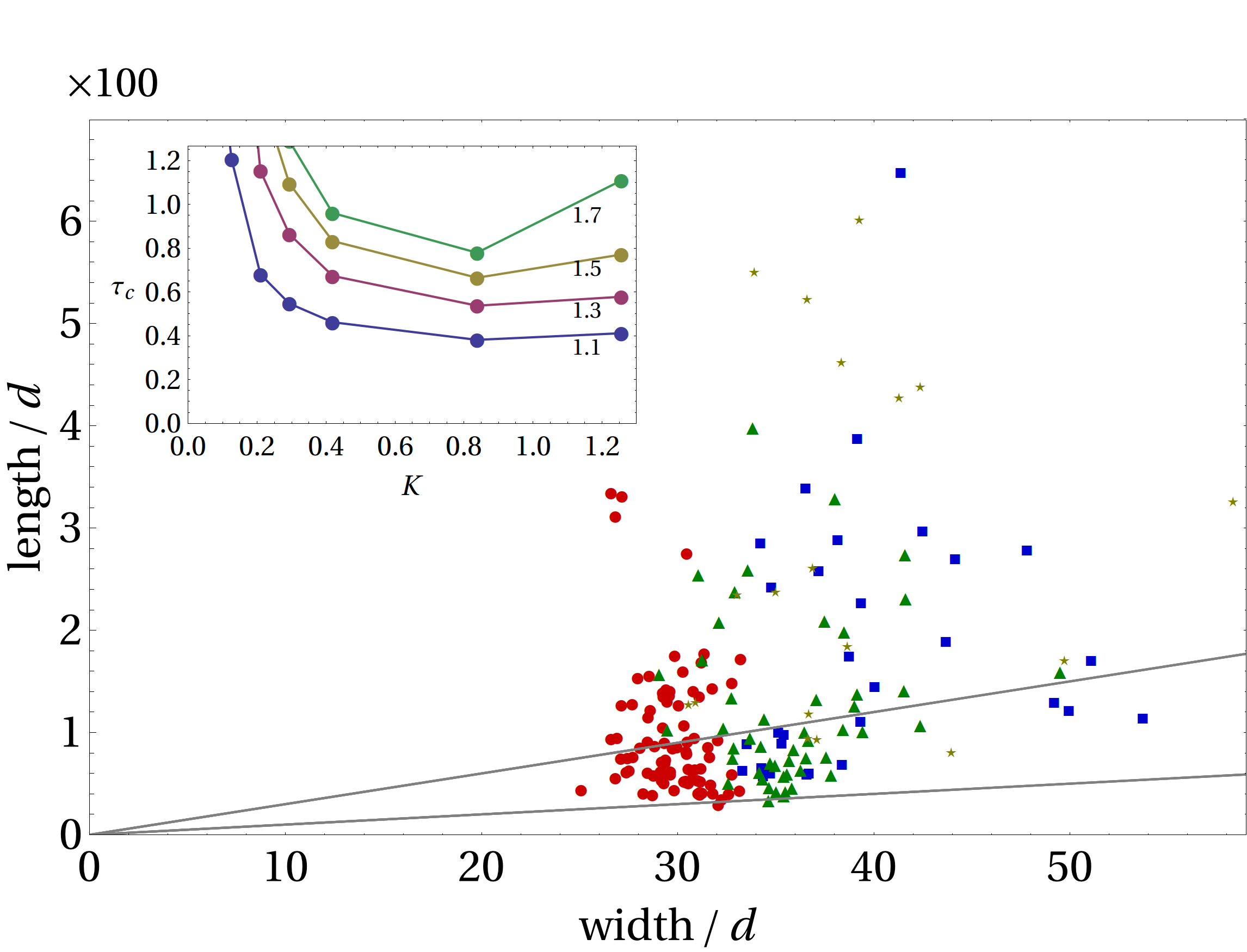
Previous findings suggest that droplet formation is due to an instability, causing small fluctuations at certain wavelengths to grow, while other wavelengths are stable. To shed light on this instability, we impose a small undulation in the initial state, follow the time evolution of the respective Fourier mode and determine the time , it takes the amplitude to grow beyond a certain value , i.e. . This result is shown in the inset of Fig. 3. A fastest growing mode can be identified and hardly depends on the choice of . In the following section, we study this instability in terms of a continuum theory and compare the predictions to simulation and experiment.
Continuum theory — To analyse the stability of the initially homogeneous stream we use continuum theory [8, 11]. Our starting point are the Navier-Stokes equations for the velocity field, , in cylindrical coordinates assuming axial symmetry
| (3) |
together with the equation of motion for the interface ,
| (4) |
Here denotes the pressure, the density and the shear viscosity. These equations have to be solved, subject to the boundary conditions, requiring the balance of normal and tangential forces at the interface: at . Here is the curvature of the interface, is the surface tension divided by the density and denotes the stress tensor.
To obtain approximate solutions to the above equations, we follow Eggers [8] and assume that variations in the radial direction take place on scales small compared to variations along the stream. Under these assumtions a one dimensional Navier Stokes equation for has been derived [8] for an incompressible fluid:
| (5) | |||||
| (6) |
These equations have been studied in various circumstances for molecular fluids [8, 11]. The best known one is the Rayleigh Plateau instability, where one expands around a state with constant radius and velocity which does not apply in the presence of gravity. Jet flow dominated by viscous effects [12, 13] has also been analysed within the above one-dimensional model. Here we consider instead a freely falling stream [14] in the comoving frame. This state is characterized by a time dependent velocity gradient, that is constant in space: . Incompressibilty requires . These fields solve the above equations exactly, allowing us to do a linear stability analysis by expanding around the above solution.
We introduce a dimensionless position variable such that remains fixed, if moves along with the stream. The -dependence can then be taken care of by plane waves: . To further simplify the notation, we introduce dimensionless time and wavenumber . We obtain two linear equations for and :
| (7) |
For clarity of presentation we have set and hence are left with one dimensionless parameter . The generalisation to finite viscosity is straighforward and given in the supplementary material [15].
The above eqs. are two ordinary differential equations with time-dependent coefficients. This makes the stability analysis complex, because a given wavenumber, which is stable at , can override an initially unstable mode in the course of time. Of course the equations can easily be integrated numerically. Before discussing the generalised eigenvalue problem, we try to extract the qualitative behaviour by inspecting the equations for small and large times. For we expect the initial strainrate to have a stabilising effect, in particular for long wavelength perturbations. For long times, , on the other hand, the strainrate decays. With the ansatz ansatz one finds for
that all wavenumbers are unstable for sufficiently large , because the dominant term is the one involving the surface tension ().
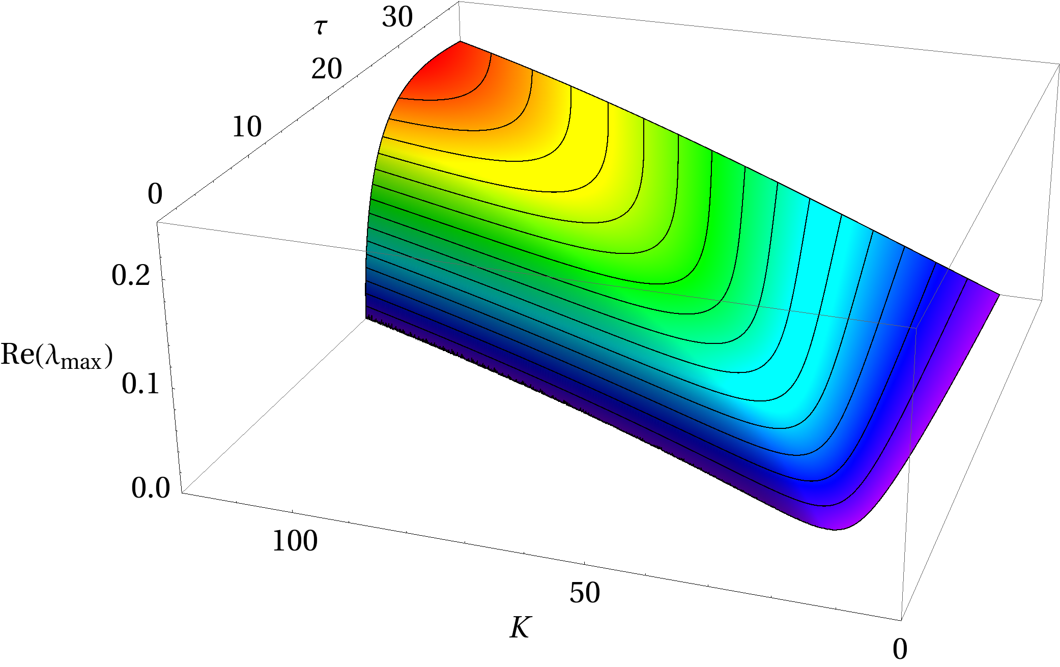
To discuss the general case, we compute the eigenvalues for all and , by diagonalising the time-dependent matrix of coefficients. The larger eigenvalue, , – responsible for the instability – is shown in Fig. 4 as a function of and in the range of values, where . The parameters for the initial strain rate, , and the surface tension, , are taken from experiment and the viscosity is set to zero. We observe that initially all wavelength are stable for , the first instability sets in at and . This wavenumber is the initially imposed one and has to be scaled down by the stretching factor , when the stream has been stretched up to time . Furthermore, wavenumbers are measured in units of the initial radius of the stream, which decreases according to . Hence to obtain the ratio of wavelength to radius at time , when the instability occurs, we have to scale wavenumbers according to . If one plots the eigenvalue versus , one observes a ridge at approximately , implying that at each instant of time – while the stream is stretching – unstable modes with roughly the wavelength of Rayleigh Plateau are growing.

However, we stress that our system is not in a stationary state, but expanding. As a consequence the eigenvalues are time dependent, and whether a perturbation increases or decreases depends on the time of its occurence. In Fig. 5 we show an example of the integrated Eqs. with 3 modes excited initially ( for ). As expected from the eigenvalue analysis, initially all modes are stable, then the smallest starts to grow, but is - at later times - overridden by the larger wavenumbers. This is meant to illustrate that the observed pattern will depend on the instant, when a fluctuation with a particular wavenumber occurs.
Variation of the parameters — If the viscosity is increased, the results remain qualitatively the same, but the instabilities occur at later times, because viscosity tends to stabilise the flow. If the initial strain rate is put to zero, we recover the Rayleigh-Plateau instability. Interesting effects are observed by varying the cohesive energy. Decreasing the cohesive energy, , the initial range of unstable wavenumbers shifts to larger , i.e. smaller wavelength in agreement with simulations (see Fig. 2). We determine the time which it takes an unstable mode of wavenumber to grow by 50% from its initial value for several values of cohesive energy. In that way we can deduce the critical wavenumber and the time for the stability to occur as a function of . These are shown in the inset of Fig. 5. We clearly observe an increase in critical wavelength with in agreement with simulation and experiment. Furthermore for increased the instability occurs earlier.
Conclusions — We have shown that a stream of granular particles
falling under gravity is generically unstable due to surface tension
– even though the Rayleigh-Plateau argument does not apply. In the
comoving frame the stream is freely expanding, implying that the
initially straight profile is subject to a time-dependent strain rate.
Linearising the Navier-Stokes equation around this nonstationary
state, we have shown that the strain rate stabilises the straight flow
profile at short times, whereas for long times all wavenumbers are
unstable. Since we expand around a nonstationary state, the growth
rate of a given wavelength depends on the time, when the corresponding
fluctuation occurs spontaneosuly or is introduced into the flow.
Thus a variety of patterns may be observed including behaviour
reminiscent of the Rayleigh-Plateau instability [5].
Acknowledgments – We are grateful to Heinrich Jaeger for suggesting to apply a model
of cohesive particles to freely falling streams. Furthermore we
acknowledge interesting discussions with him and Scott Waitukaitis
as well as financial support by the Deutsche Forschungsgemeinschaft
(DFG) through Grant Zi 209/8-01.
References
- [1] M. E. Möbius, Phys. Rev. E 74, 051304 (2006).
- [2] J. R. Royer, D. J. Evans, L. Oyarte, E. Kapit, M. Möbius, S. R. Waitukatis, and H. M. Jaeger, Nature 459, 1110 (2009).
- [3] S. R. Waitukaitis, H. F. Grütjen, J. R. Royer, and H. M. Jaeger, Phys. Rev. E 83, 051302 (2011).
- [4] Y. Amarouchene, J.-F. Boudet, and H. Kellay, Phys. Rev. Lett. 100, 218001 (2008).
- [5] G. Prado, Y. Amarouchene, and H. Kellay, Phys. Rev. Lett. 106, 198001 (2011).
- [6] S. Ulrich, T. Aspelmeier, K. Roeller, A. Fingerle, S. Herminghaus, and A. Zippelius, Phys. Rev. Lett. 102, 148002 (2009); Phys. Rev. E 80, 031306 (2009).
- [7] This is in contrast to [A. Alvarez, E. Clement and R. Soto, Phys. Fluids 18, 083301 (2006)], who inject the particles into a suspension.
- [8] J. Eggers, Rev. Mod. Phys. 69, 865 (1997).
- [9] J. S. Rowlinson, and B. Widom, Molecular Theory of Capillarity (Clarendon Press, 1982)
- [10] See supplementary material at [URL will be inserted by AIP] for a movie showing the stream’s evolution and droplet formation.
- [11] J. Eggers, and E. Villermeaux, Rep. Prog. Phys. 71, 036601 (2008).
- [12] U. S. Sauter, and H. W. Buggisch, J. Fluid Mech. 533, 237 (2005).
- [13] S. Senchenko, T. Bohr, Phys. Rev. E 71, 056301 (2005).
- [14] I. Frankel, and D. Weihs, J. Fluid Mech. 155, 289 (1985).
- [15] See supplementary material at [URL will be inserted by AIP] for the generalisation of (7).