One vertex spin-foams with the Dipole Cosmology boundary

In this subsection we recall the definition of OSN diagrams we introduced in [20]. In the analogy to spin-foams, which are colored 2-complexes, OSN-diagrams are colored graph diagrams. We first recall the definition of graph diagrams and then we recall the definition of coloring which turns a graph diagram into an OSN-diagram.

One may think of graph diagrams as a way of building 2-complexes from building blocks which are (suitable) neighborhoods of vertices of the corresponding foam [1, 18]. Such a neighborhood is a 2-complexes obtained as an image of a homotopy of a graph. When glued together, they form a 2-complex. The way one glues them together is encoded in certain relations.

Strictly speaking a graph diagram $(\mathcal{G},\mathcal{R})$ consists of a set ${\mathcal{G}}$ of oriented, connected, closed graphs $\{\Gamma_{1},...,\Gamma_{N}\}$ and a family $\mathcal{R}$ of relations defined as follows (see figure 1):

• •

  $\mathcal{R}_{\rm node}$: a symmetric relation in the set of nodes of the graphs which we call the node relation, such that each node $n$ is either in relation with precisely one $n^{\prime}\not=n$ or is unrelated (in the later case, it is called a boundary node).

• •

  $\mathcal{R}_{\rm link}$: a family of symmetric relations in the set of links of the graphs which we call collectively the link relation. If a node $n$ is in relation with a node $n^{\prime}$, then we define a bijective map between incoming/outgoing links at $n$, with outgoing/incoming links at $n^{\prime}$; no link is left free neither at the node $n$ nor at $n^{\prime}$; two links identified with each other by the bijection are called to be in the relation $\mathcal{R}^{(n,n^{\prime})}_{\rm link}$ at the pair of nodes $n,n^{\prime}$; a link which intersects $n$/$n^{\prime}$ twice, emerges in the relation twice: once as an incoming and once as an outgoing link.

In order to be related, two nodes have to satisfy the consistency condition: the number of the incoming/outgoing links at each of them has to coincide with the number of the outgoing/incoming links at the other one (with possible closed links counted twice). Note that two graphs can be treated as one disconnected graph. Thus to reduce that ambiguity we assume that all the graphs defining the diagram are connected.

An operator spin-network diagram $({\cal G}=\{\Gamma_{1},...,\Gamma_{N}\},\mathcal{R},\rho,P,A)$ is defined by using a compact group $G$ and coloring a graph diagram $({\cal G},\mathcal{R})$ as follows (see figure 1):

• •

  The coloring $\rho$ assigns to each link $\ell$ of each graph $\Gamma_{I}$, $I=1,...,N$ an irreducible representation of the group $G$:

  $$\ell\mapsto\rho_{\ell}.$$

  (1)

  It is assumed that whenever two links $\ell$ and $\ell^{\prime}$ are mapped to each other by the link relation $\mathcal{R}_{\rm link}^{nn^{\prime}}$ at some nodes $n$ and $n^{\prime}$, then

  $$\rho_{\ell}=\rho_{\ell^{\prime}}.$$

  (2)

• •

  The coloring $P$ assigns to each node $n$ an operator:

  $$n\mapsto P_{n}\in\mathcal{H}_{n}\otimes\mathcal{H}_{n}^{*},$$

  (3)

  where $\mathcal{H}_{n}$ is a Hilbert space defined at each node in the following way:

  $$\mathcal{H}_{n}\ =\ \mathrm{Inv}\left(\bigotimes_{i}\mathcal{H}_{\rho_{i}}^{*}\otimes\bigotimes_{j}\mathcal{H}_{\rho_{j}}\right)\;\subset\;\left(\bigotimes_{i}\mathcal{H}_{\rho_{i}}^{*}\otimes\bigotimes_{j}\mathcal{H}_{\rho_{j}}\right)$$

  (4)

  where $i$/$j$ labels the links incoming/outgoing at $n$.

  Whenever two nodes $n$ and $n^{\prime}$ are related by $\mathcal{R}_{\rm node}$, then (from (2) and (4)) it follows that $\mathcal{H}_{n}=\mathcal{H}_{n^{\prime}}^{*}$ and it is assumed about $P$ that

  $$P_{n}=P_{n^{\prime}}^{*}$$

  (5)

• •

  The coloring $A$ assigns to each graph $\Gamma_{I}$ a tensor, which we call contractor:

  $$\Gamma_{I}\mapsto A_{\Gamma}\in\ \left(\bigotimes_{n}{\cal H}_{n}\right)^{*}$$

  (6)

  where $n$ runs through the nodes of $\Gamma_{I}$.

Each graph $\Gamma_{I}$ itself defines a contractor, in the sense that there is a natural contraction defined by the graph $\Gamma_{I}$ and by the natural trace operation in $\bigotimes_{\ell}{\cal H}_{\ell}\otimes{\cal H}_{\ell}^{*}$ which contains $\bigotimes_{n}{\cal H}_{n}$, where $n$ / $\ell$ ranges the set of nodes/links of $\Gamma_{I}$. We denote this natural contractor by $A^{\rm Tr}_{\Gamma_{I}}$. However, that natural contraction is often preceded by some additional operations, like the EPRL embedding which gives rise to the EPRL operator spin-network diagrams.

An important element of our characterization of graph diagrams is an oriented squid set. Given a graph (oriented and closed), its oriented squid set is obtained by removing from each link of the graph a point of its entry and shaking the whole thing so that the disconnected parts of each link go apart (figure 2).

Two different graphs may define a single squid set. Therefore, it makes sense to introduce and consider the notion of a squid set on its own. An oriented squid consist of $1$ point called head, $k^{+}$ legs beginning at the head, and $k^{-}$ legs ending at the head. In other words it may be considered as the topological space obtained by glueing $k^{+}+k^{-}$ oriented intervals with the head in the suitable way (figure 3a).

An oriented squid set ${\cal S}$ is a disjoint finite union of squids (figure 3b).

A graph $\Gamma$ consists of a squid set ${\cal S}_{\Gamma}$ and information about glueing the legs of the squids. Conversely, given a squid set ${\cal S}$, a graph may be obtained by glueing the end of each outgoing leg with the beginning of arbitrarily chosen incoming leg of either the same or a different squid. However this procedure neither is unique, nor there is a guarantee it can be completed. Therefore, a single squid set can be the squid set of either more then one graph, or of an exactly one graph, or of no graph at all (figure 4).

A graph diagram $(\Gamma,{\cal R})$ can also be obtained from a squid set ${\cal S}_{\Gamma}$ by endowing it with additional structure. The part of the structure has been already described above, it allows to reconstruct the graph $\Gamma$. The second element of the structure, the node relation ${\cal R}^{\rm node}$, is given by indicating a set of pairs $\{\{\lambda_{1},\lambda^{\prime}_{1}\},...,\{\lambda_{N},\lambda^{\prime}_{N}\}\}$ of squids $\lambda_{i},\lambda^{\prime}_{i}\in{\cal S}$, whose heads are in the node relation ${\cal R}^{\rm node}$. The last element of the graph diagram structure, a link relation, is defined for each pair $\{\lambda_{i},\lambda^{\prime}_{i}\}$ as a bijection between the incoming/outgoing legs of the squid $\lambda_{i}$ with the outgoing/incoming legs of the squid $\lambda^{\prime}_{i}$ (figure 5).

This characterization of an arbitrary graph diagram leads to the following algorithm for construction of all the graph diagrams:

1. 1.

   Squids: fix a squid set ${\cal S}$ (figure 6)

   

2. 2.

   Node relation: choose $N$ pairs $\lambda_{i},\lambda^{\prime}_{i}$, $i=1,...,N$ of consistent squids (the numbers of incoming/outgoing legs of unprimed squid in each pair coincides with the numbers of the outgoing/incoming legs in the primed squid); an element $\lambda\in{\cal S}$ can emerge only once in this set of pairs or not at all (figure 7). The relation ${\cal R}_{\rm node}$ is such that the heads of the chosen squids $\lambda_{i}$ and $\lambda^{\prime}_{i}$, for $i=1,...,N$ are related to each other, and to nothing else.

   

3. 3.

   Link relation: for each pair $\lambda_{i},\lambda^{\prime}_{i}$ of the squids, $i=1,...,N$, define a bijective map carrying the incoming/outgoing legs on one squid into the outgoing/incoming legs of the other squid.

4. 4.

   Glueing: glue the end of each outgoing leg with the beginning of exactly one incoming leg of either the same or a different squid (figure 8).

   

5. 5.

   Given the data $(i)-(iii)$ perform all possible options of the glueing $(iv)$ - see figure 9.

A graph diagram ${\cal D}$ resulting from $(i)-(iv)$ consist of a graph

the disjoint union of connected graphs $\Gamma_{I}$, $I=1,..,N$ obtained by the glueing $(iv)$, a node relation given by $(ii)$ and a link relation provided by $(iii)$. We denote it shortly by ${\cal D}=(\{\Gamma_{1},...,\Gamma_{N}\},{\cal R})$. It is turned into an operator spin-network diagram by coloring the links, the nodes and the connected components of $\Gamma$ according to Section 1.1.

In [20] (see Sec. 6.2), for every graph $\Gamma$ we introduced the graph diagram corresponding to the static spin-foam, that is the spin-foam describing the trivial evolution of the graph. Let us denote this diagram by ${\cal D}_{\Gamma}$ and refer to it as the static graph diagram of $\Gamma$. The boundary of ${\cal D}_{\Gamma}$ is the disjoint union $\Gamma\cup\bar{\Gamma}$ where $\bar{\Gamma}$ is a graph obtained by switching the orientation of each of the links of $\Gamma$ (figure 10).

Given a coloring of the links of the graph $\Gamma$ by representations, we endow the static graph diagram ${\cal D}_{\Gamma}$ with the natural colorings (see [20], Sec. 6.2): $(i)$ the coloring $\rho$ of the links of the graphs in ${\cal D}_{\Gamma}$ is the one induced by the coloring of the links of $\Gamma$; $(ii)$ the operator coloring $P$ colors with the identity operators; $(iii)$ finally, all the contractor coloring $A$ assigns to each $n$-theta graph of ${\cal D}_{\Gamma}$ the natural trace contractor $A^{\rm Tr}$. The result is the static OSN-diagram. The corresponding operator is the identity in the Hilbert space given by the coloring of the links of $\Gamma$. The technical definition of static diagram will be recalled in the next subsection.

The diagrams we will construct with the improved algorithm introduced below, contain the boundary $\Gamma$ together with its static diagram ${\cal D}_{\Gamma}$ as a subdiagram. Given $\Gamma$, our construction will provide all the diagrams of this type, that is all the diagrams, modulo the static sub-diagram. In terms of the spin-foam formalism, we will construct all the spin-foams bounded by an arbitrarily fixed graph $\Gamma$. In each of the spin-foams, the neighborhood of $\Gamma$ is homeomorphic to the cylinder $\Gamma\times$ $[0,1]$.

The key trick behind our construction is the following observation: given a graph $\Gamma$ of the squid set ${\cal S}_{\Gamma}$, and an arbitrary graph diagram ${\cal D}_{\rm int}$ called interaction diagram, whose boundary graph $\partial{\cal D}_{\rm int}$ has the same squid set:

we can combine the diagram ${\cal D}_{\rm int}$ with the static diagram ${\cal D}_{\Gamma}$ into the new graph diagram ${\cal D}_{\Gamma}\#{\cal D}_{\rm int}$ such that the graph $\Gamma$ becomes its boundary. We achieve that by defining the graph of ${\cal D}_{\Gamma}\#{\cal D}_{\rm int}$ to be the disjoint union of the graph of ${\cal D}_{\Gamma}$ with the graph of ${\cal D}_{\rm int}$ and extending the node and link relations of the component diagrams such that each squid of the boundary ${\partial\cal D}_{\rm int}$ is related to the corresponding squid of $\bar{\Gamma}$ (a part of the boundary of ${\cal D}_{\Gamma}$) - see figure 11.

The identification of the squid sets ${\cal S}_{\Gamma}$ and $\partial{\cal D}$ is defined modulo symmetries of ${\cal S}_{\Gamma}$ (exchanging identical squids). In the consequence, the graphs $\bar{\Gamma}$ and $\partial{\cal D}_{\rm int}$ may admit more than one way of relating their squid. In the algorithm below, the identification (a bijection) between the squid sets will be given, and the freedom will be in the glueing of the legs.

Below we implement this idea in detail, beginning with recalling the exact definition of the static diagrams.

First, we recall the definition of the static diagram of a graph $\Gamma$. We use the squid set ${\cal S}_{\Gamma}$. For each squid $\lambda\in{\cal S}_{\Gamma}$ we introduce a theta-like graph $\tilde{\theta}_{\lambda}$ as follows (figure 12):

• •

  $\bar{\lambda}$: we introduce a new squid $\bar{\lambda}$ obtained by flipping the orientation of each of the legs of $\lambda$.

• •

  $\theta_{\lambda}$: glue each outgoing/incoming leg $\ell_{\lambda,i}$ of $\lambda$ with the corresponding incoming/outgoing leg ${\ell}_{\bar{\lambda},i}$ of $\bar{\lambda}$ to obtain a link ${\ell}_{\bar{\lambda},i}\circ\ell_{\lambda,i}$ / $\ell_{\lambda,i}\circ{\ell_{\bar{\lambda},i}}$ connecting the head $n_{\lambda}$ of the squid $\lambda$ with the head ${n}_{\bar{\lambda}}$ of the squid $\bar{\lambda}$; the result is a closed graph $\theta_{\lambda}$.

• •

  $\tilde{\theta}_{\lambda}$: on each link $\bar{\ell}_{\lambda,i}\circ\ell_{\lambda,i}$ / $\ell_{\lambda,i}\circ\bar{\ell}_{\lambda,i}$ we introduce an extra node $n_{\lambda,i}$; the resulting graph is denoted $\tilde{\theta}_{\lambda}$

The links of the graph $\tilde{\theta}_{\lambda}$ are just the legs $\ell_{\lambda,i}$, $\bar{\ell}_{\lambda,i}$, $i=1,2,...$ of the squids $\lambda$ and $\bar{\lambda}$ respectively.

The result of this procedure is a family of the graphs $\tilde{\theta}_{\lambda}$, one per each squid $\lambda\in{\cal S}_{\Gamma}$. The disjoint union $\coprod_{\lambda}\tilde{\theta}_{\lambda}$ is the graph of the static graph diagram ${\cal D}_{\Gamma}$. The node and the link relations in $\coprod_{\lambda}\tilde{\theta}_{\lambda}$ are induced by the the structure of the graph $\Gamma$ - see figure 13.

To define the node relation, notice that the set of the nodes of the graph $\coprod_{\lambda}\tilde{\theta}_{\lambda}$ consists of the nodes of two types:

• •

  The first type is the heads of the squids $\lambda\in{\cal S}_{\Gamma}$ (denoted by $n_{\lambda}$) and the heads of the conjugate squids $\bar{\lambda}$ (denoted by $n_{\bar{\lambda}},...$) - those nodes are left unrelated by the node relation, that is they become the boundary nodes.

• •

  The ends of the legs of the squids $\lambda\in{\cal S}_{\Gamma}$ (glued with the legs of the conjugate squids $\bar{\lambda}$) denoted by $n_{\ell_{\lambda,i}}$. Whenever $\ell_{\lambda,i}\circ\ell^{\prime}_{\lambda^{\prime},i^{\prime}}$ is a link of $\Gamma$, then the nodes $n_{\ell_{\lambda,i}}$ and $n_{\ell^{\prime}_{\lambda^{\prime},i^{\prime}}}$ are in the node relation.

The link relation is defined as follows:

• •

  For every pair of the nodes $n_{\ell_{\lambda,i}}$ and $n_{\ell^{\prime}_{\lambda^{\prime},i^{\prime}}}$ related above by the node relation, each node is two-valent. The link relation is defined to pair the links $\ell_{\lambda,i}$ and $\ell^{\prime}_{\lambda^{\prime},i^{\prime}}$, as well as the links $\ell_{\bar{\lambda},i}$ and $\ell^{\prime}_{\bar{\lambda}^{\prime},i^{\prime}}$ (see the previous item).

Given a static graph diagram ${\cal D}_{\Gamma}$ the natural coloring consists of: irreducible representations freely assigned to the links, the operators $P_{n_{\lambda}}={\rm id}:{\cal H}_{n_{\lambda}}\rightarrow{\cal H}_{n_{\lambda}}$ for every head $n_{\lambda}$ and every squid $\lambda$, and $P_{n_{\ell_{\lambda,i}}n_{\ell^{\prime}_{\lambda^{\prime},i^{\prime}}}}$ equal to the natural isomorphisms ${\rm id}:{\cal H}_{n_{\ell_{\lambda,i}}}\rightarrow{\cal H}_{n_{\ell^{\prime}_{\lambda^{\prime},i^{\prime}}}}$. Finally, the contractor assigned to each component graph $\tilde{\theta}_{\lambda}$ is the natural $A^{\rm Tr}_{\tilde{\theta}}$.

We present now our algorithm for the construction of the operator spin-network diagrams whose unoriented boundary is an arbitrarily fixed unoriented graph $|\Gamma|$.

1. 1.

   $\Gamma$: choose an orientation of each link of $|\Gamma|$, the result is an oriented graph $\Gamma$ (figure 14).

   

2. 2.

   ${\cal S}_{\rm int}$: to the squid set ${\cal S}_{\Gamma}$ of the graph $\Gamma$ add $N$ pairs of squids $\lambda_{1},\lambda^{\prime}_{1},...,\lambda_{N},\lambda^{\prime}_{N}$, such that for each pair the number of incoming/outgoing legs of one squid equals the number of outgoing/incoming legs of the other one (figure 15). Denote the resulting squid set ${\cal S}_{\rm int}$. Introduce a node relation by relating the head of $\lambda_{i}$ with the head of $\lambda^{\prime}_{i}$, $i=1,...,N$.

   

   

3. 3.

   ${\cal D}_{\rm int}$: To the squid set ${\cal S}_{\rm int}$ with the chosen set of pairs of the squids $\lambda_{1},\lambda^{\prime}_{1},...,\lambda_{N},\lambda^{\prime}_{N}$ and the node relation apply the steps $(iii)$ and $(iv)$ of the algorithm of section 2.2. Denote the resulting graph diagram ${\cal D}_{\rm int}$ (figure 16).

   

   

4. 4.

   ${\cal D}_{\Gamma}\#{\cal D}_{\rm int}$: Use the static graph diagram ${\cal D}_{\Gamma}$ of the graph $\Gamma$ and construct the union of the diagrams as it was explained above (figure 17).

   

   

5. 5.

   Coloring: Define arbitrary coloring of the diagram ${\cal D}_{\Gamma}\#{\cal D}_{\rm int}$ which turns it into operator an spin-network diagram (figure 18).

   

   

6. 6.

   Consider all possible: orientations of $|\Gamma|$, $N$-tuples of pairs of squids added to ${\cal S}_{\Gamma}$, ways of connecting the legs of ${\cal S}_{\rm int}$, link relations for each $\lambda_{i},\lambda^{\prime}_{i}$, colorings in $(v)$.

Notice, that it would be insufficient to fix one orientation of the boundary. A priori all the orientations have to be taken into account. On the other hand, in general, the algorithm will possibly give OSN-diagrams related by the reorientation (see the previous section). In specific cases, that redundancy should be reduced. The presented construction allows to control the level of complexity of resulting diagram by the level of complexity of the diagram ${\cal D}_{\rm int}$. The complexity can be measured by the number of pairs of the nodes related by the node relation, that is the number of internal edges. The simplest case is zero internal edges, that is the squid set

In that case all the graph used to define graph diagram ${\cal D}_{\rm int}$ becomes the boundary graph $\partial{\cal D}_{\rm int}$.

A general example of the interaction graph diagram ${\cal D}_{\rm int}$ is given by a graph $\tilde{\Gamma}_{\rm int}$ and a node relation ${\cal R}_{\rm int}^{\rm node}$ consisting of exactly $N$ pairs of nodes. Increasing the number $N$ we increase the complexity of the diagram ${\cal D}_{\Gamma}\#{\cal D}_{\rm int}$.

In the previous subsection we have recalled the structure of colorings that turn graph diagrams into operator spin-network diagrams. In the case of the graph diagrams constructed in this subsection, without lack of generality, it is sufficient to consider colorings of the diagrams ${\cal D}_{\Gamma}\#{\cal D}_{\rm int}$ provided by our algorithm, which reduced to the static graph diagram ${\cal D}_{\Gamma}$ provides the static operator spin-network diagram defined above. A way to control the freedom in the colorings by representations is to fix a coloring of the links of the boundary graph $\Gamma$.

In the next section we apply the algorithm to construct all the operator spin-network diagrams of the Rovelli-Vidotto dipole cosmology.

We apply now the algorithm of the previous section to construct all the operator spin-network diagrams whose boundary is fixed (modulo an orientation) to be the graph $|\Gamma|$ which consists of two disjoint $4$-valent theta graphs $|\Gamma_{4\theta}|$ (figure 19),

and which correspond to 1-vertex spin-foams.

In terms of the improved algorithm of the previous section this assumption means that the the interaction diagram ${\cal D}_{\rm int}$ consists of one graph $\Gamma_{\rm int}$ whereas the node and link relations are trivial. That is its squid set equals the squid set of the boundary (the initial plus the final) graph. Specifically, for this Dipole Cosmology example and with the 1-vertex assumption the improved algorithm from section 3.3 reads:

1. 1.

   $\Gamma$: choose an orientation of each link of each of the two graphs $|\Gamma_{4\theta}|$ (figure 20a).

   (a)

   (b)

   (c)

2. 2.

   ${\cal S}_{\rm int}={\cal S}_{\Gamma}$: for the interaction squid set take the squid set ${\cal S}_{\Gamma}$ of the graph $\Gamma$; this means that in point $(ii)$ of the general algorithm presented in section 3.3 we set $N=0$ – in other words, we consider the first order of the vertex and edge expansion; the interaction squid set consists of four $4$-valent squids; two of them are oriented freely - their orientation determines the orientation of the remaining two squids and defines the orientation of $\Gamma$ (figure 20b).

3. 3.

   $\Gamma_{\rm int}$: glue each incoming/outgoing leg of each squid of ${\cal S}_{\rm int}$ with an outgoing/incoming leg of another (or the same) squid of ${\cal S}_{\rm int}$. In the next subsection we construct and list all the possible (unoriented) interaction graphs (they are depicted later, on figure 27). $\Gamma_{\rm int}$ is obtained by assigning orientation to each link of one such graph (figure 20c). Together with the trivial node and link relations, $\Gamma_{\rm int}$ defines an interaction graph ${\cal D}_{\rm int}$.

4. 4.

   ${\cal D}_{\Gamma}\#{\cal D}_{\rm int}$: Use the static graph diagram ${\cal D}_{\Gamma}$ of the graph $\Gamma$ (figure 21a) and construct the union of the diagrams as it was explained above (figure 21b).

   (a)

   (b)

5. 5.

   Coloring: Define arbitrary coloring of the diagram ${\cal D}_{\Gamma}\#{\cal D}_{\rm int}$ which turns it into an operator spin-network diagram.

6. 6.

   Consider all the possible: orientations of the two independent squids of ${\cal S}_{\Gamma}$, ways of connecting the legs of the four squids, all possible node relations between the nodes of the interaction graph and corresponding nodes of static diagram, all possible link relations between the links of the interaction graph and the corresponding links of the static diagram.

In this subsection we construct all the possible interaction graphs $\Gamma_{\rm int}$. We obtain each interaction graph $\Gamma_{\rm int}$ by assigning an orientation to each link of an (unoriented) graph $|\Gamma_{\rm int}|$ defined by the following two properties:

• •

  each graph $|\Gamma_{\rm int}|$ has exactly 4 nodes,

• •

  each node of $|\Gamma_{\rm int}|$ is precisely four-valent.

We find below all possible graphs $|\Gamma_{\rm int}|$. We depicted the resulting graphs on figure 27. In order to obtain an interaction graph $\Gamma_{\rm int}$, we assign to each link of a graph $|\Gamma_{\rm int}|$ an orientation consistent with the orientation of the boundary (and the squid set). Given a graph $|\Gamma_{\rm int}|$ and (oriented) boundary graph $\Gamma$, such a choice of compatible orientation may be impossible. For example, take graph 1 from figure 27 as a graph $|\Gamma_{\rm int}|$. It is not possible to choose an orientation of links of this graph compatible with orientation of the boundary graph from figure 20a. This is because the boundary graph figure 20a has a node with three outgoing and one incoming link and such a structure of a node is not possible for graph 1 from figure 27 (since each link of this graph forms a loop, the number of incoming links and outgoing links needs to be equal at every node). Note, that there is a distinguished graph $|\Gamma_{\rm int}|$ – the graph 20 from figure 27 used in [21]. This graph may be oriented in a way compatible with any boundary graph $\Gamma$. The natural question which arises is whether for every graph from figure 27 there is a boundary graph such that orientation of $|\Gamma_{\rm int}|$ may be chosen to be compatible with this boundary graph. The answer is affirmative. It may be shown that orientation of links of each graph $|\Gamma_{\rm int}|$ may be chosen to be compatible with a boundary graph oriented such that at every node a number of incoming links equals to a number of outgoing links.

We now present in details the construction of unoriented graphs possessing exactly 4 nodes, all of which are four-valent, i.e. all possible graphs $|\Gamma_{\rm int}|$. It is well known that each unoriented graph may be encoded in adjacency matrix. It is a symmetric matrix $A\in{\rm Sym}(n)$ with the number of columns/rows $n$ equal to the number of the vertices of this graph. The entries $A_{ij}$ are equal to the numbers of links connecting node $i$ with node $j$, with a specification that links forming closed loops (corresponding to diagonal entries) are counted twice. An example of such matrix and the corresponding graph is given on figure 22.

However, given a graph there are many corresponding matrices, because for each permutation $\sigma\in{\rm S}_{n}$ the matrices

and $A_{ij}$ define the same graph. There is a natural bijective correspondence between graphs with $n$ vertices and orbits, elements of ${\rm Sym}(n)/S_{n}$.

In our case graphs have four nodes. We are therefore interested in $4\times 4$ matrices. The condition that each node is 4-valent corresponds to an assumption that the sum of numbers in each row/column is equal 4:

The set of the possible interaction graphs $\mathcal{G}_{\rm int}$ is therefore characterised by the moduli space:

First we introduce a parametrisation of the space of symmetric matrices satisfying (13) and then we find the moduli space using Wolfram‘s Mathematica 8.0.

To define our parametrisation in a transparent way, we introduce a triple $({\rm K}_{4},d,m)$ (see figure 23):

• •

  the complete graph ${\rm K}_{4}$ on four nodes – the skeleton of a 4-simplex (we denote by ${\rm K}_{4}^{(0)}$ the set of its nodes and by ${\rm K}_{4}^{(1)}$ the set of its links);

• •

  labeling of its nodes

  $$d:{\rm K}_{4}^{(0)}\ni n\mapsto d_{n}\in\{0,2,4\}$$

  (15)

  such that for all four nodes $n_{1},\,n_{2},\,n_{3},\,n_{4}$ of the graph ${\rm K}_{4}$ the numbers $d_{n_{1}},\,d_{n_{2}},\,d_{n_{3}},\,d_{n_{4}}$ satisfy the generalized triangle inequalities:

  $$\forall_{i}\ d_{n_{i}}\leq\sum_{i\not=j}d_{n_{j}}.$$

  (16)

• •

  labeling of its links

  $$m:{\rm K}_{4}^{(1)}\ni\ell\mapsto m_{\ell}\in\{0,1,2,3,4\}$$

  (17)

  such that

  $$\forall_{n\in{\rm K}_{4}^{(0)}}\ \sum_{\{\ell\in{\rm K}_{4}^{(1)}:\ell\cap n\not=\emptyset\}}m_{\ell}=d_{n}$$

  (18)

The condition that $d_{n},\ n\in{\rm K}_{4}^{(0)}$ satisfy the generalized triangle inequalities (16) ensures the existence of at least one labeling $m$¹¹ 1 This well known fact is used for example in the representation theory of SU(2) to construct of the invariants of the tensor product $\mathcal{H}_{{d_{n_{1}}}/{2}}\otimes\mathcal{H}_{{d_{n_{2}}}/{2}}\otimes\mathcal{H}_{{d_{n_{3}}}/{2}}\otimes\mathcal{H}_{{d_{n_{4}}}/{2}}$, where dim$\,\mathcal{H}_{j}=2j+1$, and $d_{n_{1}}+...+d_{n_{4}}\in 2\mathbb{N}$ by the construction.

To each triple $({\rm K}_{4},d,m)$ corresponds a (multi)graph $\Gamma_{({\rm K}_{4},d,m)}$, defined in the following way (see also an example at figure 24):

• •

  it has the same set of nodes $\Gamma_{({\rm K}_{4},d,m)}^{(0)}={\rm K}_{4}^{(0)};$

• •

  for each pair $(n,n^{\prime})$ of different nodes there are exactly $m_{\ell}$ links of $\Gamma_{({\rm K}_{4},d,m)}$ connecting the nodes $n$ and $n^{\prime}$, where $\ell$ is the link of $K_{4}$ connecting $n$ with $n^{\prime}$ .

• •

  at each node $n$ there are precisely $(4-d_{n})/2$ links each of which makes a loop connecting $n$ with itself (figure 25);

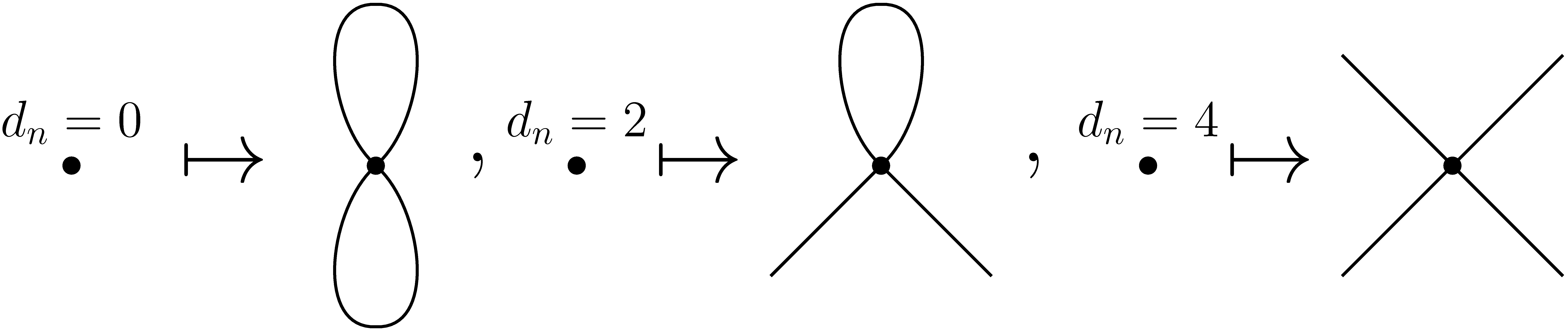
Alternatively one may read from $({\rm K}_{4},d,m)$ the corresponding adjacency matrix.

Simply choose some ordering of nodes (in our case it is a labelling of nodes with numbers $\{1,2,3,4\}$) and let $\ell_{ij}=\ell_{ji},\ i\not=j$ be the link in K₄ connecting nodes $n_{i}$ and $n_{j}$. Now

• •

  terms $4-d_{n_{i}}$ correspond to diagonal entries of the adjacency matrix,i.e. $A_{\underline{i}\underline{i}}:=4-d_{n_{i}}$,

• •

  terms $m_{\ell_{ij}}$ correspond to off-diagonal entries, i.e. $A_{ij}:=m_{\ell_{ij}}$ for $i\not=j$.

This correspondence is depicted on figure 26. Note that, having known the numbers $d_{n}$, the total number of links going from nodes $n_{1},\,n_{2}$ to nodes $n_{3},\,n_{4}$ (we denote it by $k$) and the number $m_{\ell_{23}}$, we can reconstruct the remaining coloring of $({\rm K}_{4},d,m)$. As a result those numbers give the parametrisation of adjacency matrix, we are using. Explicitly, we parametrize the solutions to equations (13) with

• •

  four numbers $d_{1},\,d_{2},\,d_{3},\,d_{4}\in\{0,2,4\}$ satisfying triangle inequalities (16),

• •

  a natural number $k\in\left[|d_{1}-d_{2}|,d_{1}+d_{2}\right]\cap\left[|d_{3}-d_{4}|,d_{3}+d_{4}\right]$, such that $k+d_{1}+d_{2}\in 2\mathbb{N}$,

• •

  an even natural number $m\in\left[d_{3}-d_{4}+d_{2}-d_{1},{\rm min}\{d_{3}-d_{4}+k,d_{2}-d_{1}+k\}\right]$.

The corresponding parametrisation is:

We next find orbits of action of permutation group $S_{4}$ on the set of those solutions. To this end we used Mathematica 8.0. The resulting graphs are depicted on figure 27.

Note that one could further restrict the number of matrices considered by requiring that the sequence $(d_{1},\,d_{2},\,d_{3},\,d_{4})$ is monotonous and considering only orbits under action of $S_{4}/H$, where $H$ is the subgroup, which does not change the sequence $(d_{1},\,d_{2},\,d_{3},\,d_{4})$. This remark enables one to do the calculation without using computer. On the other hand, one could write a program which does not use the parametrisation we introduced – e.g. one could generate matrices with entries taking values in the set $\{0,1,2,3,4\}$ (with even numbers on diagonal) and choose only those which satisfy equation (13) (a direct method). We have chosen the method we present here, because it gives better understanding of the structure of the graphs considered, it is less laborious than calculation by hand and the version we used is easier to implement than the direct method. It has the additional advantage that it is easily applicable to a more general case where the four nodes are not necessarily four-valent. When $d_{1},\,d_{2},\,d_{3},\,d_{4}$ are becoming larger, this method becomes considerably faster than the direct method.

As we explained in the previous subsection, there are exactly 20 interaction graphs. However, the number of the graph diagrams resulting from the procedure described above is different. In this subsection we discuss in more details the diversity of the resulting graph diagrams.

Given an oriented interaction graph ${\cal D}_{\rm int}$ and a static diagram ${\cal D}_{\Gamma}$, there may be more than one graph diagrams ${\cal D}_{\Gamma}\#{\cal D}_{\rm int}$. The ambiguity is in the choice of the node relation and the link relations.

• •

  The ambiguity in node relation. It exists if an oriented interaction graph $\Gamma_{\rm int}$ has two nodes, say $n_{1}$ and $n_{2}$, such that the number of the incoming/outgoing links at $n_{1}$ is equal to the number of the incoming/outgoing links at $n_{2}$. Then, for every node relation between the nodes of the interaction graph and the corresponding nodes of the static diagram, there is another, different node relation obtained by switching the nodes $n_{1}$ and $n_{2}$ – see figure 28.

  

  

• •

  The ambiguity in link relations. Having settled down the node relation, there are still many possible link relations. The only condition, that each link relation needs to satisfy, is that incoming/outgoing link at each node in interaction graph is in relation with outgoing/incoming link at corresponding node in the static diagram (see figure 29).

  

  

Furthermore, some colorings of the boundary links may be incompatible with some interaction graphs – it may happen that the amplitude is zero for every coloring of a given interaction graph. In order to see how this limits the number of possible interaction graphs, consider the coloring of boundary graph depicted on figure 30a and OSN diagram on figure 30b (node relations and the corresponding coloring with operators is omitted for clarity). It is straightforward to see that the amplitude is non-zero only if the representations $\rho_{2}$ and $\rho_{3}$ and, respectively, the representations $\rho_{1}$ and $\rho_{5}$ are equal ($\rho_{2}=\rho_{3}$, $\rho_{1}=\rho_{5}$). Importantly, note that, because there are links forming closed loops in the interaction graph, the amplitude is non-zero only if among representations $\rho_{1},\,\rho_{2},\,\rho_{3},\,\rho_{4}$ or among representations $\rho_{5},\,\rho_{6},\,\rho_{7},\,\rho_{8}$ there is a pair of equal representations. In addition, since the interaction graph is connected the amplitude is non-zero only if there is a pair of equal representations $\rho_{i}=\rho_{j}$, such that $i\in\{1,2,3,4\},\,j\in\{5,6,7,8\}$. Those two conditions do not depend on the choice of node and link relations but on the structure of interaction graph only. This example shows that there are colorings of boundary graph which are not compatible with the given interaction graph.

A similar analysis may be performed for other interaction graphs. It leads to an interesting conclusion. There is a distinguished interaction graph, which is not limited by the coloring in the way described above – it is the graph 20 from figure 27 used in [21]. The corresponding amplitude is non-zero even if all eight links of the boundary graph are labeled with pairwise different representations. In this generic case, all other interaction graphs give identically zero amplitude. We expect therefore that for a generic boundary state (which is a linear combination of spin-network states of all possible spins), the graph diagram with this interaction graph gives major contribution. This conclusion needs however further justification.

References

- [1]
Reisenberger MP (1994) World sheet formulations of gauge theories and gravity, (Preprint arXiv:gr-qc/9412035)
Reisenberger MP, Rovelli C (1997) ’’Sum over Surfaces‘‘ form of Loop Quantum Gravity, Phys.Rev.D56,3490-3508 (Preprint arXiv:gr-qc/9612035v) - [2] Baez J (2000) An introduction to Spinfoam Models of BF Theory and Quantum Gravity, Lect.Notes Phys.543,25-94 (Preprint arXiv:gr-qc/9905087v1)
- [3] Perez A (2003) Spinfoam models for Quantum Gravity, Class.Quant.Grav.20,R43 (Preprint arXiv:gr-qc/0301113v2)
- [4] Rovelli C (2004) Quantum Gravity, (Cambridge: Cambridge University Press)
- [5] Bahr B, Hellmann F, Kamiński W, Kisielowski M, Lewandowski J (2010) Operator Spin Foam Models, Class.Quant.Grav.28,105003,2011 (Preprint arXiv:1010.4787v1)
- [6] Ashtekar A, Lewandowski J (2004) Background independent quantum gravity: A status report, Class.Quant.Grav.21,R53 (Preprint arXiv:gr-qc/0404018)
- [7] Muxin Han, Weiming Huang, Yongge Ma (2007) Fundamental Structure of Loop Quantum Gravity, Int.J.Mod.Phys.D16,1397-1474 (Preprint arXiv:gr-qc/0509064)
- [8] Ashtekar A (1991) Lectures on Non-perturbative Canonical Gravity, (Notes prepared in collaboration with R.S. Tate), (World Scientific Singapore)
- [9] Thiemann T (2007) Introduction to Modern Canonical Quantum General Relativity, (Cambridge: Cambridge University Press)
- [10]
Rovelli C, Smolin C (1995) Discreteness of area and volume in quantum gravity, Nucl.Phys.B442,593 [(1995) Erratum-ibid. B456 753] (Preprint arXiv:gr-qc/9411005)
Ashtekar A, Lewandowski J (1995) Differential Geometry on the Space of Connections via Graphs and Projective Limits, J.Geom.Phys.17,191-230 (Preprint arXiv:hep-th/9412073)
Ashtekar A, Lewandowski J (1997) Quantum theory of geometry. I: Area operators, Class.Quant.Grav.14,A55 (Preprint arXiv:gr-qc/9602046)
Ashtekar A, Lewandowski J (1998) Quantum theory of geometry. II: Volume operators, Adv.Theor.Math.Phys.1,388 (Preprint arXiv:gr-qc/9711031)
Thiemann T (1998) A length operator for canonical quantum gravity, J.Math.Phys.39,3372 (Preprint arXiv:gr-qc/9606092) - [11] Barrett JW, Crane L (1998) Relativistic spin-networks and quantum gravity, J.Math.Phys.39,3296-3302 (Preprint arXiv:gr-qc/9709028)
- [12] Engle J, Livine E, Pereira R, Rovelli C (2008) LQG vertex with finite Immirzi parameter, Nucl.Phys.B799,136-149 (Preprint arXiv:0711.0146v2)
- [13]
Engle J, Pereira R, Rovelli C (2008) Flipped spinfoam vertex and loop gravity, Nucl.Phys.B798,251-290 (Preprint arXiv:0708.1236v1)
Livine ER, Speziale S (2007) A new spinfoam vertex for quantum gravity, Phys.Rev.D76,084028 (Preprint arXiv:0705.0674v2) - [14]
Freidel L, Krasnov K (2008) A New Spin Foam Model for 4d Gravity, Class.Quant.Grav.25,125018 (Preprint arXiv:0708.1595v2)
Livine ER, Speziale S (2008) Consistently Solving the Simplicity Constraints for Spinfoam Quantum Gravity, Europhys.Lett.81,50004 (Preprint arXiv:0708.1915)
Bojowald M, Perez A (2010) Spin foam quantization and anomalies, Gen.Rel.Grav.42,877-907 (Preprint arXiv:gr-qc/0303026) - [15] Muxin H, Thiemann T (2010) Commuting Simplicity and Closure Constraints for 4D Spin Foam Models, (Preprint arXiv:1010.5444)
- [16] Ding Y, Muxin H, Rovelli C (2011) Generalized Spinfoams, Phys. Rev. D83 124020
- [17] Engle J (2011) A proposed proper EPRL vertex amplitude, (Preprint arXiv:1111.2865) Engle J (2012) A spin-foam vertex amplitude with the correct semiclassical limit, (Preprint arXiv:1201.2187)
- [18] Kamiński W, Kisielowski M, Lewandowski J (2010) Spin-Foams for All Loop Quantum Gravity, Class.Quantum Grav.27,095006 (Preprint arXiv:0909.0939v2)
- [19] Hellmann F (2011) State Sums and Geometry, PhD Thesis University of Nottingham (Preprint arXiv:1102.1688v1)
- [20] Kisielowski M, Lewandowski J, Puchta J (2012) Feynman diagrammatic approach to spinfoams ,Class. Quantum Grav.29 015009 (Preprint arXiv:1107.5185v1
- [21] Bianchi E, Rovelli C, Vidotto F (2010) Towards Spinfoam Cosmology, Phys.Rev.D82,084035,2010 (Preprint arXiv:1003.3483v1)