On the Influence of Informed Agents on Learning and Adaptation over Networks

Sheng-Yuan Tu Ali H. Sayed ^†^†thanks: This work was supported in part by NSF grants CCF-1011918 and CCF-0942936. A short conference version of this work appears in [1]. The authors are with the Department of Electrical Engineering, University of California, Los Angeles (e-mail: shinetu@ee.ucla.edu; sayed@ee.ucla.edu)

Abstract

Adaptive networks consist of a collection of agents with adaptation and learning abilities. The agents interact with each other on a local level and diffuse information across the network through their collaborations. In this work, we consider two types of agents: informed agents and uninformed agents. The former receive new data regularly and perform consultation and in-network tasks, while the latter do not collect data and only participate in the consultation tasks. We examine the performance of adaptive networks as a function of the proportion of informed agents and their distribution in space. The results reveal some interesting and surprising trade-offs between convergence rate and mean-square performance. In particular, among other results, it is shown that the performance of adaptive networks does not necessarily improve with a larger proportion of informed agents. Instead, it is established that the larger the proportion of informed agents is, the faster the convergence rate of the network becomes albeit at the expense of some deterioration in mean-square performance. The results further establish that uninformed agents play an important role in determining the steady-state performance of the network, and that it is preferable to keep some of the highly connected agents uninformed. The arguments reveal an important interplay among three factors: the number and distribution of informed agents in the network, the convergence rate of the learning process, and the estimation accuracy in steady-state. Expressions that quantify these relations are derived, and simulations are included to support the theoretical findings. We further apply the results to two models that are widely used to represent behavior over complex networks, namely, the Erdos-Renyi and scale-free models.

Index Terms:

Adaptive networks, diffusion adaptation, learning, network topology, Erdos-Renyi model, scale-free model, power-law distribution, small-world phenomenon, informed agents, uninformed agents, convergence rate, mean-square performance.

I Introduction

Adaptive networks consist of a collection of spatially distributed nodes that are linked together through a connection topology and that cooperate with each other through local interactions. Adaptive networks are well-suited to perform decentralized information processing and inference tasks [2, 3] and to model complex and self-organized behavior encountered in biological systems [4, 5], such as fish joining together in schools [6] and birds flying in formation [7].

In previous works on adaptive networks [2, 3, 6], and in other related studies on distributed and combination algorithms [8, 9, 10, 11, 12, 13, 14, 15, 16, 17, 18, 19, 20, 21], the agents are usually assumed to be homogeneous in that they all have similar processing capabilities and are able to have continuous access to information and measurements. However, it is generally observed in nature that the behavior of a biological network is often driven more heavily by a small fraction of the agents as happens, for example, with bees and fish [22, 23, 24]. This phenomenon motivates us to study in this paper adaptive networks where only a fraction of the nodes are assumed to be informed, while the remaining nodes are uninformed. Informed nodes collect data regularly and perform in-network processing tasks, while uninformed nodes only participate in consultation tasks in the manner explained in the sequel.

We shall examine how the transient and steady-state behavior of the network are dependent on its topology and on the proportion of the informed nodes and their distribution in space. The results will reveal some interesting and surprising trade-offs between convergence rate and mean-square performance. In particular, among other results, the analysis will show that the performance of adaptive networks does not necessarily improve with a larger proportion of informed nodes. Instead, it is discovered that the larger the proportion of informed nodes is, the faster the convergence rate of the network becomes albeit at the expense of some deterioration in mean-square performance. The results also establish that uninformed nodes play an important role in determining the steady-state performance of the network, and that it is preferable to maintain some of the highly connected nodes uninformed. The analysis in the paper reveals the important interplay that exists among three factors: the number of informed nodes in a network, the convergence rate of the learning process, and the estimation accuracy. We shall further apply the results to two topology models that are widely used in the complex network literature [25], namely, the Erdos-Renyi and scale-free models.

To establish the aforementioned results, a detailed mean-square-error analysis of the network behavior is pursued. However, the difficulty of the analysis is compounded by the fact that nodes interact with each other and, therefore, they influence each other’s learning process and performance. Nevertheless, for sufficiently small step-sizes, we will be able to derive an expression for the network’s mean-square deviation (MSD). By examining this expression, we will establish that the MSD is influenced by the eigen-structure of two matrices: the covariance matrix representing the data statistical profile and the combination matrix representing the network topology. We then study the eigen-structure of these matrices and derive useful approximate expressions for their eigenvalues and eigenvectors. The expressions are subsequently used to reveal that the network MSD can be decomposed into two components. We study the behavior of each component as a function of the proportion of informed nodes; both components show important differences in their behavior. When the components are added together, a picture emerges that shows how the performance of the network depends on the proportion of informed nodes in an manner that supports analytically the popular wisdom that more information is not necessarily better [26].

The organization of the paper is as follows. In Sections II and III, we review the diffusion adaptation strategy and establish conditions for the mean and mean-square stability of the networks in the presence of uninformed nodes. In Section IV, we introduce two popular models from the complex network literature. In Section V, we analyze in some detail the structure of the mean-square performance of the networks and reveal the effect of the network topology and node distribution on learning and adaptation. Simulation results appear in Section V in support of the theoretical findings.

II Diffusion Adaptation Strategy

Consider a collection of $N$ nodes distributed over a domain in space. Two nodes are said to be neighbors if they can share information. The set of neighbors of node $k$ , including $k$ itself, is called the neighborhood of $k$ and is denoted by $\mathcal{N}_{k}$ . The nodes would like to estimate some unknown column vector, $w^{\circ}$ , of size $M$ . At every time instant, $i$ , each node $k$ is able to observe realizations $\{d_{k}(i),u_{k,i}\}$ of a scalar random process $\boldsymbol{d}_{k}(i)$ and a $1\times M$ vector random process $\boldsymbol{u}_{k,i}$ with a positive-definite covariance matrix, $R_{u,k}=\mathbb{E}\boldsymbol{u}_{k,i}^{*}\boldsymbol{u}_{k,i}>0$ , where $\mathbb{E}$ denotes the expectation operator. All vectors in our treatment are column vectors with the exception of the regression vector, $\boldsymbol{u}_{k,i}$ , which is taken to be a row vector for convenience of presentation. The random processes $\{\boldsymbol{d}_{k}(i),\boldsymbol{u}_{k,i}\}$ are assumed to be related to $w^{\circ}$ via a linear regression model of the form [27]:

\boldsymbol{d}_{k}(i)=\boldsymbol{u}_{k,i}w^{\circ}+\boldsymbol{v}_{k}(i)

(1)

where $\boldsymbol{v}_{k}(i)$ is measurement noise with variance $\sigma^{2}_{v,k}$ and assumed to be spatially and temporally independent with

\mathbb{E}\boldsymbol{v}^{*}_{k}(i)\boldsymbol{v}_{l}(j)=\sigma^{2}_{v,k}\cdot\delta_{kl}\cdot\delta_{ij}

(2)

in terms of the Kronecker delta function. The noise $\boldsymbol{v}_{k}(i)$ is assumed to be independent of $\boldsymbol{u}_{l,j}$ for all $l$ and $j$ . The regression data $\boldsymbol{u}_{k,i}$ is likewise assumed to be spatially and temporally independent. All random processes are assumed to be zero mean. Note that we use boldface letters to denote random quantities and normal letters to denote their realizations or deterministic quantities. Models of the form (1)-(2) are useful in capturing many situations of interest, such as estimating the parameters of some underlying physical phenomenon, or tracking a moving target by a collection of nodes, or estimating the location of a nutrient source or predator in biological networks (see, e.g., [6, 7]).

The objective of the network is to estimate $w^{\circ}$ in a distributed manner through an online learning process, where each node is allowed to interact only with its neighbors. The nodes estimate $w^{\circ}$ by seeking to minimize the following global cost function:

J^{\text{glob}}(w)\triangleq\sum_{k=1}^{N}\mathbb{E}|\boldsymbol{d}_{k}(i)-\boldsymbol{u}_{k,i}w|^{2}

(3)

Several diffusion adaptation schemes for solving (3) in a distributed manner were proposed in [2, 3, 28]; the latter reference considers more general cost functions. It was shown in these references, through a constructive stochastic approximation and incremental argument, that the structure of a near-optimal distributed solution for (3) takes the form of the Adapt-then-Combine (ATC) strategy of [3]; this strategy can be shown to outperform other strategies in terms of mean-square performance including consensus-based strategies [29, 30]. Hence, we focus in this work on ATC updates. The ATC strategy operates as follows. We select an $N\times N$ left-stochastic matrix $A$ with nonnegative entries $\{a_{l,k}\geq 0\}$ satisfying:

A^{T}\mathds{1}=\mathds{1}\text{ and }a_{l,k}=0\text{ if, and only if, $l\notin\mathcal{N}_{k}$}

(4)

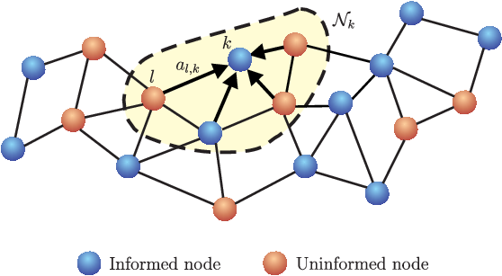
where $\mathds{1}$ is a vector of size $N$ with all entries equal to one. The entry $a_{l,k}$ denotes the weight on the link connecting node $l$ to node $k$ , as shown in Fig. 1. Thus, condition (4) states that the weights on all links arriving at node $k$ add up to one. Moreover, if two nodes $l$ and $k$ are linked, then their corresponding entry $a_{l,k}$ is positive; otherwise, $a_{l,k}$ is zero. The ATC strategy consists of two steps. The first step (5a) involves local adaptation, where node $k$ uses its own data $\{d_{k}(i),u_{k,i}\}$ . This step updates the weight estimate at node $k$ from $w_{k,i-1}$ to an intermediate value $\psi_{k,i}$ . The second step (5b) is a combination (consultation) step where the intermediate estimates $\{\psi_{l,i}\}$ from the neighborhood are combined through the weights $\{a_{l,k}\}$ to obtain the updated weight estimate $w_{k,i}$ . The ATC strategy is described as follows:

		$\displaystyle\psi_{k,i}=w_{k,i-1}+\mu_{k}u_{k,i}^{*}[d_{k}(i)-u_{k,i}w_{k,i-1}]$			(5a)
		$\displaystyle w_{k,i}=\sum_{l\in\mathcal{N}_{k}}a_{l,k}\psi_{l,i}$			(5b)

where $\mu_{k}$ is the positive step-size used by node $k$ . To model uninformed nodes over the network, we shall set $\mu_{k}=0$ if node $k$ is uninformed. We assume that the network contains at least one informed node. In this model, uninformed nodes do not collect data $\{d_{k}(i),u_{k,i}\}$ and, therefore, do not perform the adaptation step (5a); they, however, continue to perform the combination or consultation step (5b). In this way, informed nodes have access to data and participate in the adaptation and consultation steps, whereas uninformed nodes play an auxiliary role through their participation in the consultation step only. This participation is nevertheless important because it helps diffuse information across the network. One of the main contributions of this work is to examine how the proportion of informed nodes, and how the spatial distribution of these informed nodes, influence the learning and adaptation abilities of the network in terms of its convergence rate and mean-square performance. It will follow from the analysis that uninformed nodes also play an important role in determining the network performance.

Refer to caption — Fig. 1: A connected network with informed and uninformed nodes. The weight $a_{l,k}$ scales the data transmitted from node $l$ to node $k$ over the edge linking them.

III Network Mean-Square Performance

The mean-square performance of ATC networks has been studied in detail in [3] for the case where all nodes are informed. Expressions for the network performance, and conditions for its mean-square stability, were derived there by applying energy conservation arguments [27, 31]. In this section, we start by showing how to extend the results to the case in which only a fraction of the nodes are informed. The condition for mean-square stability will need to be properly adjusted as explained below in (13) and (14). We start by examining mean stability.

III-A Mean Stability

Let the error vector for any node $k$ be denoted by:

\tilde{\boldsymbol{w}}_{k,i}\triangleq w^{\circ}-\boldsymbol{w}_{k,i}

(6)

We collect all weight error vectors and step-sizes across the network into a block vector and block matrix:

\displaystyle\tilde{\boldsymbol{w}}_{i}\triangleq\text{col}\left\{\tilde{\boldsymbol{w}}_{1,i},\cdots,\tilde{\boldsymbol{w}}_{N,i}\right\},\quad\mathcal{M}\triangleq\text{diag}\{\mu_{1}I_{M},\cdots,\mu_{N}I_{M}\}

(7)

where the notation $\text{col}\{\cdot\}$ denotes the vector that is obtained by stacking its arguments on top of each other, and $\text{diag}\{\cdot\}$ constructs a diagonal matrix from its arguments. We also introduce the extended combination matrix:

\mathcal{A}\triangleq A\otimes I_{M}

(8)

where the symbol $\otimes$ denotes the Kronecker product of two matrices. Then, starting from (5a)-(5b) and using model (1), some algebra will show that the global error vector in (7) evolves according to the recursion:

\boxed{\tilde{\boldsymbol{w}}_{i}=\mathcal{A}^{T}(I_{NM}-\mathcal{M}\boldsymbol{\mathcal{R}}_{i})\tilde{\boldsymbol{w}}_{i-1}-\mathcal{A}^{T}\mathcal{M}\boldsymbol{s}_{i}}

(9)

where

\displaystyle\boldsymbol{\mathcal{R}}_{i}\triangleq\text{diag}\{\boldsymbol{u}^{*}_{1,i}\boldsymbol{u}_{1,i},\cdots,\boldsymbol{u}^{*}_{N,i}\boldsymbol{u}_{N,i}\},\quad\boldsymbol{s}_{i}\triangleq\text{col}\{\boldsymbol{u}^{*}_{1,i}\boldsymbol{v}_{1,i},\cdots,\boldsymbol{u}^{*}_{N,i}\boldsymbol{v}_{N,i}\}

(10)

Since the regressors $\{\boldsymbol{u}_{k,i}\}$ are spatially and temporally independent, then the $\{\boldsymbol{u}_{k,i}\}$ are independent of $\tilde{\boldsymbol{w}}_{i-1}$ . Taking expectation of both sides of (9), we find that the mean relation for $\tilde{\boldsymbol{w}}_{i}$ evolves in time according to the recursion:

\boxed{\mathbb{E}\tilde{\boldsymbol{w}}_{i}=\mathcal{B}\cdot\mathbb{E}\tilde{\boldsymbol{w}}_{i-1}}

(11)

where we introduced the block matrices:

\displaystyle\mathcal{B}\triangleq\mathcal{A}^{T}(I_{NM}-\mathcal{M}\mathcal{R}),\quad\mathcal{R}\triangleq\mathbb{E}\boldsymbol{\mathcal{R}}_{i}=\text{diag}\{R_{u,1},\cdots,R_{u,N}\}

(12)

In the following statement, we provide conditions to ensure mean stability of the network, namely, that $\mathbb{E}\tilde{\boldsymbol{w}}_{i}\rightarrow 0$ as $i\rightarrow\infty$ , even in the presence of uninformed nodes.

Theorem 1 (Mean stability).

The ATC network (5b) with at least one informed node converges in the mean sense if the step-sizes $\{\mu_{k}\}$ and the combination matrix $A$ satisfy the following two conditions:

1.

For every informed node $l$ , its step-size $\mu_{l}$ satisfies:

$0<\mu_{l}\cdot\rho(R_{u,l})<2$ (13)

where the notation $\rho(\cdot)$ denotes the spectral radius of its matrix argument.
2.

There exists a finite integer $j$ such that for every node $k$ , there exists an informed node $l$ satisfying:

$\left[A^{j}\right]_{l,k}>0$ (14)

That is, the $(l,k)$ th entry of $A^{j}$ is positive. [This condition essentially ensures that there is a path from node $l$ to node $k$ in $j$ steps.]

Proof.

We first introduce a block matrix norm. Let $\Sigma$ be an $N\times N$ block matrix with blocks of size $M\times M$ each. Its block matrix norm, $\|\Sigma\|_{b}$ , is defined as:

\|\Sigma\|_{b}\triangleq\max_{1\leq k\leq N}\left(\sum_{l=1}^{N}\|\Sigma_{k,l}\|_{2}\right)

(15)

where $\Sigma_{k,l}$ denotes the $(k,l)$ th block of $\Sigma$ and $\|\cdot\|_{2}$ denotes the largest singular value of its matrix argument. That is, we first compute the 2-induced norm of each block $\Sigma_{k,l}$ and then find the $\infty$ -norm of the $N\times N$ matrix formed from the entries $\{\|\Sigma_{k,l}\|_{2}\}$ . It can be verified that (15) satisfies the four conditions for a matrix norm [32]. To prove mean stability of the ATC network (5b), we need to show that conditions (13)-(14) guarantee $\rho(\mathcal{B})<1$ , or equivalently, $\rho(\mathcal{B}^{j})<1$ for any $j$ . Now, note that

\displaystyle\rho(\mathcal{B}^{j})\leq\|\mathcal{B}^{j}\|_{b}=\max_{1\leq k\leq N}\left(\sum_{l=1}^{N}\left\|\left[\mathcal{B}^{j}\right]_{k,l}\right\|_{2}\right)

(16)

By the rules of matrix multiplication, the $(k,l)$ th block (of size $M\times M$ ) of the matrix $\mathcal{B}^{j}$ is given by:

\left[\mathcal{B}^{j}\right]_{k,l}=\sum_{m_{1}=1}^{N}\sum_{m_{2}=1}^{N}\cdots\sum_{m_{j-1}=1}^{N}\mathcal{B}_{k,m_{1}}\mathcal{B}_{m_{1},m_{2}}\cdots\mathcal{B}_{m_{j-1},l}

(17)

where $\mathcal{B}_{k,l}$ is the $(k,l)$ th block (of size $M\times M$ ) of the matrix $\mathcal{B}$ from (12) and is given by

\mathcal{B}_{k,l}=a_{l,k}\cdot(I_{M}-\mu_{l}R_{u,l})

(18)

Then, using the triangle inequality and the submultiplicative property of norms, the 2-induced norm of $[\mathcal{B}^{j}]_{k,l}$ in (17) is bounded by:

\displaystyle\left\|\left[\mathcal{B}^{j}\right]_{k,l}\right\|_{2}\leq\sum_{m_{1}=1}^{N}\sum_{m_{2}=1}^{N}\cdots\sum_{m_{j-1}=1}^{N}\|\mathcal{B}_{k,m_{1}}\|_{2}\cdot\|\mathcal{B}_{m_{1},m_{2}}\|_{2}\cdots\|\mathcal{B}_{m_{j-1},l}\|_{2}

(19)

Note that in the case where $l\in\mathcal{N}_{m}$ , we obtain from condition (13) and expression (18) that

\displaystyle\|\mathcal{B}_{m,l}\|_{2}=a_{l,m}\cdot\rho\left(I_{M}-\mu_{l}R_{u,l}\right)\begin{cases}<a_{l,m},&\text{if node $l$ is informed}\\ =a_{l,m},&\text{if node $l$ is uninformed}\end{cases}

(20)

where we replaced the 2-induced norm with the spectral radius because covariance matrices are Hermitian. Relation (20) and condition (4) imply that

\displaystyle\left\|\left[\mathcal{B}^{j}\right]_{k,l}\right\|_{2}\leq\sum_{m_{1}=1}^{N}\sum_{m_{2}=1}^{N}\cdots\sum_{m_{j-1}=1}^{N}a_{m_{1},k}\cdot a_{m_{2},m_{1}}\cdots a_{l,m_{j-1}}

(21)

Strict inequality holds in (21) if, and only if, the sequence $(l,m_{j-1},\ldots,m_{1},k)$ forms a path from node $l$ to node $k$ using $j$ edges and there exists at least one informed node along the path. Since we know from condition (14) that there is an informed node, say, node $l^{\circ}$ , such that a path with $j$ edges exists from node $l^{\circ}$ to node $k$ , we then get from (16) and (21) that

$\displaystyle\rho(\mathcal{B}^{j})$	$\displaystyle\leq\max_{1\leq k\leq N}\left(\left\\|\left[\mathcal{B}^{j}\right]_{k,l^{\circ}}\right\\|_{2}+\sum_{l\neq l^{\circ}}\left\\|\left[\mathcal{B}^{j}\right]_{k,l}\right\\|_{2}\right)$	(22)
	$\displaystyle<\max_{1\leq k\leq N}\sum_{l=1}^{N}\left(\sum_{m_{1}=1}^{N}\sum_{m_{2}=1}^{N}\cdots\sum_{m_{j-1}=1}^{N}a_{m_{1},k}\cdot a_{m_{2},m_{1}}\cdots a_{l,m_{j-1}}\right)$
	$\displaystyle=\max_{1\leq k\leq N}\sum_{l=1}^{N}\left[A^{j}\right]_{l,k}$
	$\displaystyle=1$

where the last equality is from condition (4) because $(A^{T})^{j}\mathds{1}=\mathds{1}$ if $A^{T}\mathds{1}=\mathds{1}$ . ∎

Condition (14) is satisfied if the matrix $A$ is primitive [32]. Since, by (4), $A$ is left-stochastic, it follows from the Perron-Frobenius Theorem [32] that the eigen-structure of $A$ satisfies certain prominent properties, which will be useful in the sequel, namely, that (a) $A$ has an eigenvalue at $\lambda=1$ ; (b) the eigenvalue at $\lambda=1$ has multiplicity one; (c) all the entries of the right and left eigenvectors associated with $\lambda=1$ are positive; and (d) $\rho(A)=1$ so that all other eigenvalues of $A$ have magnitude strictly less than one. We remark that since in this paper we will be dealing with connected networks (where a path always exists between any two arbitrary nodes), then condition (14) is automatically satisfied. As such, the ATC strategy (5b) will converge in the mean whenever there exists at least one informed node with its step-size satisfying condition (13). In the next section, we show that conditions (13)-(14) further guarantee mean-square convergence of the network when the step-sizes are sufficiently small.

III-B Mean-Square Stability

The network mean-square-deviation (MSD) is used to assess how well the network estimates the weight vector, $w^{\circ}$ . The MSD is defined as follows:

\text{MSD}\triangleq\lim_{i\rightarrow\infty}\frac{1}{N}\sum_{k=1}^{N}\mathbb{E}\|\tilde{\boldsymbol{w}}_{k,i}\|^{2}

(23)

where $\|\cdot\|$ denotes the Euclidean norm for vectors. To arrive at an expression for the MSD, we first derive a variance relation for the ATC network; the variance relation indicates how the weighted mean-square error vector evolves over time [27]. Let $\Sigma$ denote an arbitrary nonnegative-definite Hermitian matrix that we are free to choose, and let $\sigma=\text{vec}(\Sigma)$ denote the vector that is obtained by stacking the columns of $\Sigma$ on top of each other. We shall interchangeably use the notation $\|x\|^{2}_{\Sigma}$ and $\|x\|^{2}_{\sigma}$ to denote the same weighted square quantity, $x^{*}\Sigma x$ . Following the energy conservation approach of [27, 31], we can motivate the following weighted variance relation:

\displaystyle\mathbb{E}\|\tilde{\boldsymbol{w}}_{i}\|^{2}_{\Sigma}=\mathbb{E}\left(\|\tilde{\boldsymbol{w}}_{i-1}\|^{2}_{(I_{NM}-\boldsymbol{\mathcal{R}}_{i}\mathcal{M})\mathcal{A}\Sigma\mathcal{A}^{T}(I_{NM}-\mathcal{M}\boldsymbol{\mathcal{R}}_{i})}\right)+\text{Tr}(\Sigma\mathcal{A}^{T}\mathcal{M}\mathcal{S}\mathcal{M}\mathcal{A})

(24)

where

\displaystyle\mathcal{S}\triangleq\mathbb{E}\boldsymbol{s}_{i}\boldsymbol{s}_{i}^{*}=\text{diag}\{\sigma^{2}_{v,1}R_{u,1},\ldots,\sigma^{2}_{v,N}R_{u,N}\}

(25)

Relation (24) can be derived from (9) directly by multiplying both sides from the left by $\tilde{\boldsymbol{w}}^{*}_{i}\Sigma$ and taking expectations. Some algebra will then show that for sufficiently small step-sizes, expression (24) can be approximated and rewritten as (see [3] for similar details, where terms that depend on higher-order powers of the small step-sizes are ignored):

\boxed{\mathbb{E}\|\tilde{\boldsymbol{w}}_{i}\|^{2}_{\sigma}=\mathbb{E}\|\tilde{\boldsymbol{w}}_{i-1}\|^{2}_{F\sigma}+\left[\text{vec}(\mathcal{Y}^{T})\right]^{T}\sigma}

(26)

where

\boxed{\mathcal{F}\triangleq\mathcal{B}^{T}\otimes\mathcal{B}^{*},\quad\mathcal{Y}\triangleq\mathcal{A}^{T}\mathcal{M}\mathcal{S}\mathcal{M}\mathcal{A}}

(27)

Relation (26) is very useful and it can be used to study the transient behavior of the ATC network, as well as its steady-state performance. The following result ensures that $\mathbb{E}\|\tilde{\boldsymbol{w}}_{i}\|^{2}_{\sigma}$ remains bounded and converges to some constant as $i$ goes to infinity.

Theorem 2 (Mean-square stability).

The ATC network (5b) with at least one informed node is mean-square stable if the step-sizes $\{\mu_{k}\}$ and the combination matrix $A$ satisfy conditions (13)-(14), and the step-sizes $\{\mu_{k}\}$ are sufficiently small such that higher-order powers of them can be ignored.

Proof.

Expression (26) holds for sufficiently small step-sizes. As shown in [3], the mean-square convergence of (26) is guaranteed if $\rho\left(F\right)<1$ . But since

\displaystyle\rho\left(\mathcal{F}\right)=\rho\left(\mathcal{B}^{T}\otimes\mathcal{B}^{*}\right)=\left[\rho\left(\mathcal{B}\right)\right]^{2}

(28)

and conditions (13)-(14) guarantee $\rho\left(\mathcal{B}\right)<1$ from Theorem 1, it also holds that $\rho\left(\mathcal{F}\right)<1$ . ∎

III-C Mean-Square Performance

Now, assume the network is mean-square stable and let the time index $i$ tend to infinity. From (26), we obtain the steady-state relation

\lim_{i\rightarrow\infty}\mathbb{E}\|\tilde{\boldsymbol{w}}_{i}\|^{2}_{\left(I_{N^{2}M^{2}}-\mathcal{F}\right)\sigma}=\left[\text{vec}(\mathcal{Y}^{T})\right]^{T}\sigma

(29)

Since the eigenvalues of the matrix $\mathcal{F}$ are within the unit disc, the matrix $\left(I_{N^{2}M^{2}}-\mathcal{F}\right)$ is invertible. Thus, the network MSD, as given by (23), can be obtained by choosing $\sigma=\left(I_{N^{2}M^{2}}-\mathcal{F}\right)^{-1}\text{vec}(I_{NM})/N$ , which leads to the following useful expression

\boxed{\begin{aligned} \text{MSD}=\frac{1}{N}\left[\text{vec}(\mathcal{Y}^{T})\right]^{T}\left(I_{N^{2}M^{2}}-\mathcal{F}\right)^{-1}\text{vec}(I_{NM})\end{aligned}}

(30)

Expression (30) relates the network MSD to the quantities $\{\mathcal{Y},\mathcal{F}\}$ defined by (27). These quantities contain information about the data statistical profile, the spatial distribution of informed nodes, and the network topology through their dependence on $\{\mathcal{R},\mathcal{M},\mathcal{A}\}$ . Using the following equalities for arbitrary matrices $\{U,W,\Sigma\}$ of compatible dimensions:

\displaystyle\text{vec}(U\Sigma W)=(W^{T}\otimes U)\sigma,\quad\text{Tr}(\Sigma W)=\left[\text{vec}(W^{T})\right]^{T}\sigma

(31)

and the fact that, for any stable matrix $F$ , it holds:

\displaystyle(I_{N^{2}M^{2}}-\mathcal{F})^{-1}

\displaystyle=\sum_{j=0}^{\infty}\mathcal{F}^{j}

(32)

we can obtain an alternative expression for the network MSD from (27) and (30), namely,

\boxed{\begin{aligned} \text{MSD}=\frac{1}{N}\sum_{j=0}^{\infty}\text{Tr}[\mathcal{B}^{j}\mathcal{Y}(\mathcal{B}^{*})^{j}]\end{aligned}}

(33)

This expression for the MSD will be the starting point for our analysis further ahead, when we examine the influence of the proportion of informed nodes on network performance.

III-D Convergence Rate

We denote the convergence rate of the ATC strategy (5b) by $r$ so that the smaller the value of $r$ is, the faster the rate of convergence of $\mathbb{E}\|\tilde{\boldsymbol{w}}_{i}\|^{2}$ is towards its steady-state value. As indicated by (26), the convergence rate is determined by the spectral radius of the matrix $F$ in (27), i.e.,

\boxed{r=\rho(\mathcal{F})=\left[\rho(\mathcal{B})\right]^{2}}

(34)

Let $\mathcal{N}_{I}$ denote the set of informed nodes, i.e., $k\in\mathcal{N}_{I}$ if node $k$ is informed. From now on, we introduce the assumption below, which essentially assumes that all informed nodes have similar processing abilities in that they use the same step-size value while observing processes arising from the same statistical distribution.

Assumption 1.

Assume that $\mu_{k}=\mu$ for all informed nodes and that the covariance matrices across all nodes are also uniform, i.e., $R_{u,k}=R_{u}$ . We continue to assume that the step-size is sufficiently small so that it holds that $0<\mu\cdot\rho(R_{u})<1$ .

Then, we have the following useful result.

Lemma 1 (Faster convergence rate).

Consider two configurations of the same network: one with $\mathcal{N}_{I,1}$ informed nodes and another with $\mathcal{N}_{I,2}$ informed nodes. Let $r_{1}$ and $r_{2}$ denote the corresponding convergence rates for these two informed configurations. If $\mathcal{N}_{I,2}\supseteq\mathcal{N}_{I,1}$ , then $r_{2}\leq r_{1}$ .

Proof.

Under Assumption 1, we have that

\displaystyle I_{M}-\mu_{l}R_{u,l}=\begin{cases}I_{M}-\mu R_{u},&\text{if node $l$ is informed}\\ I_{M},&\text{if node $l$ is uninformed}\end{cases}

(35)

Then, the matrix $[\mathcal{B}^{j}]_{k,l}$ in (17) can be written as:

\displaystyle\left[\mathcal{B}^{j}\right]_{k,l}=\sum_{m_{1}=1}^{N}\sum_{m_{2}=1}^{N}\cdots\sum_{m_{j-1}=1}^{N}a_{m_{1},k}\cdot a_{m_{2},m_{1}}\cdots a_{l,m_{j-1}}\cdot(I_{M}-\mu R_{u})^{q_{l,k}}

(36)

where the exponent $q_{l,k}$ denotes the number of informed nodes along the path $(l,m_{j-1},\ldots,m_{1},k)$ . Note that $[\mathcal{B}^{j}]_{k,l}$ is a nonnegative-definite matrix because $(I_{M}-\mu R_{u})>0$ in view of the condition $0<\mu\rho(R_{u})<1$ . In fact, all eigenvalues of $(I_{M}-\mu R_{u})$ lie within the line segment $(0,1)$ . Moreover, since $\mathcal{N}_{I,1}\subseteq\mathcal{N}_{I,2}$ , we have that $q^{(1)}_{l,k}\leq q^{(2)}_{l,k}$ and, therefore, the matrix difference

	$\displaystyle\left[\mathcal{B}^{(1)j}\right]_{k,l}-\left[\mathcal{B}^{(2)j}\right]_{k,l}=$	$\displaystyle\sum_{m_{1}=1}^{N}\sum_{m_{2}=1}^{N}\cdots\sum_{m_{j-1}=1}^{N}a_{m_{1},k}\cdot a_{m_{2},m_{1}}\cdots a_{l,m_{j-1}}$		(37)
		$\displaystyle\times\left[\left(I-\mu R_{u}\right)^{q^{(1)}_{l,k}}-\left(I-\mu R_{u}\right)^{q^{(2)}_{l,k}}\right]$		(37)

is a nonnegative-definite matrix, where the superscripts denote the indices of the informed configurations, $\mathcal{N}_{I,1}$ or $\mathcal{N}_{I,2}$ . Since $[\mathcal{B}^{(1)j}]_{k,l}$ , $[\mathcal{B}^{(2)j}]_{k,l}$ , and $[\mathcal{B}^{(1)j}]_{k,l}-[\mathcal{B}^{(2)j}]_{k,l}$ are all nonnegative-definite, then it must hold that

\left\|\left[\mathcal{B}^{(1)j}\right]_{k,l}\right\|_{2}\geq\left\|\left[\mathcal{B}^{(2)j}\right]_{k,l}\right\|_{2}

(38)

Relation (38) can be established by contradiction. Suppose that (38) does not hold, i.e., $\rho([\mathcal{B}^{(1)j}]_{k,l})<\rho([\mathcal{B}^{(2)j}]_{k,l})$ as $[\mathcal{B}^{(1)j}]_{k,l}$ and $[\mathcal{B}^{(2)j}]_{k,l}$ are Hermitian from (36). In addition, let $x$ denote the eigenvector that is associated with the largest eigenvalue of $[\mathcal{B}^{(2)j}]_{k,l}$ , i.e., $([\mathcal{B}^{(2)j}]_{k,l})x=\rho([\mathcal{B}^{(2)j}]_{k,l})x$ . Then, we obtain the following contradiction to the nonnegative-definiteness of $[\mathcal{B}^{(1)j}]_{k,l}-[\mathcal{B}^{(2)j}]_{k,l}$ :

x^{*}\left(\left[\mathcal{B}^{(1)j}\right]_{k,l}-\left[\mathcal{B}^{(2)j}\right]_{k,l}\right)x=x^{*}\left(\left[\mathcal{B}^{(1)j}\right]_{k,l}\right)x-\rho\left(\left[\mathcal{B}^{(2)j}\right]_{k,l}\right)x^{*}x<0

(39)

by the Rayleigh-Ritz Theorem [32]. By the definition of the block matrix norm in (15), we arrive at

\left(\left\|\left[\mathcal{B}^{(1)j}\right]\right\|_{b}\right)^{1/j}\geq\left(\left\|\left[\mathcal{B}^{(2)j}\right]\right\|_{b}\right)^{1/j}

(40)

for all $j$ . Let $j$ tend to infinity and we obtain that

\rho\left(\mathcal{B}^{(1)}\right)\geq\rho\left(\mathcal{B}^{(2)}\right)

(41)

where we used the fact that $\rho(\mathcal{B})=\lim_{j\rightarrow\infty}(\|\mathcal{B}^{j}\|)^{1/j}$ for any matrix norm [32]. ∎

The result of Lemma 1 shows that if we enlarge the set of informed nodes, the convergence rate decreases and convergence becomes faster. The following result provides bounds for the convergence rate.

Lemma 2 (Bound on convergence rate).

The convergence rate is bounded by

\left[1-\mu\cdot\lambda_{M}(R_{u})\right]^{2}\leq r<1

(42)

where $\lambda_{M}(R_{u})$ denotes the smallest eigenvalue of $R_{u}$ .

Proof.

Since the ATC network is mean-square stable, i.e., $\rho(\mathcal{B})<1$ , the upper bound is obvious. On the other hand, from Lemma 1, the value of $\rho(\mathcal{B})$ achieves its minimum value when all nodes are informed, i.e., the matrix $\mathcal{M}$ in (7) becomes $\mathcal{M}=\mu I_{NM}$ . In this case, the matrix $\mathcal{B}$ in (12) can be written as:

\mathcal{B}^{\circ}=A^{T}\otimes(I_{M}-\mu R_{u})

(43)

where the superscript is used to denote the matrix $\mathcal{B}$ when all nodes are informed. Then,

	$\displaystyle\rho(\mathcal{B})$	$\displaystyle\geq\rho(\mathcal{B}^{\circ})$		(44)
		$\displaystyle=\rho(A^{T})\cdot\rho(I_{M}-\mu R_{u})$		(44)

We already know that $\rho(A^{T})=1$ . In addition, because $(I_{M}-\mu R_{u})>0$ , we have that

\rho(I_{M}-\mu R_{u})=1-\mu\cdot\lambda_{M}(R_{u})

(45)

and we arrive at the lower bound in (42). ∎

IV Two Network Topology Models

Before examining the effect of informed nodes on network performance, we pause to introduce two popular models that are widely used in the study of complex networks. We shall call upon these models later to illustrate the theoretical findings of the article. For both models, we let $n_{k}$ denote the degree (number of neighbors) of node $k$ . Note that since node $k$ is a neighbor of itself, we have $n_{k}\geq 1$ . In addition, we assume the network topology is symmetric so that if node $l$ is a neighbor of node $k$ , then node $k$ is also a neighbor of node $l$ .

IV-A Erdos-Renyi Model

In the Erdos-Renyi model [33], there is a single parameter called edge probability and is denoted by $p\in[0,1]$ . The edge probability specifies the probability that two distinct nodes are connected. In this way, the degree distribution of any node $k$ becomes a random variable and is distributed according to a binomial distribution, i.e.,

f(n_{k})=\begin{pmatrix}N-1\\ n_{k}-1\end{pmatrix}p^{n_{k}-1}(1-p)^{N-n_{k}}

(46)

The expected degree for node $k$ , denoted by $\bar{n}_{k}$ , is then

\bar{n}_{k}=(N-1)p+1

(47)

Note that, in this model, all nodes have the same expected degree since the right-hand side is independent of $k$ . Therefore, the expected network degree, $\bar{\eta}$ , becomes

\bar{\eta}\triangleq\frac{1}{N}\sum_{k=1}^{N}\bar{n}_{k}=(N-1)p+1

(48)

IV-B Scale-Free Model

The Erdos-Renyi model does not capture several prominent features of real networks such as the small-world phenomenon and the power-law degree distribution [25]. The small-world phenomenon refers to the fact that the number of edges between two arbitrary nodes is small on average. The power-law degree distribution refers to the fact that the number of nodes with degree $n_{k}$ falls off as an inverse power of $n_{k}$ , namely,

f(n_{k})\sim cn_{k}^{-\gamma}

(49)

with two positive constants $c$ and $\gamma$ . Networks with degree distributions of the form (49) are called scale-free networks [34] and can be generated using preferential attachment models. We briefly describe the model proposed by [35]. The model starts with a small connected network with $N_{0}$ nodes. At every iteration, we add a new node, which will connect to $m\leq N_{0}$ distinct nodes besides itself. The probability of connecting to a node is proportional to its degree. As time evolves, nodes with higher degree are more likely to be connected to new nodes. Eventually, there are a few nodes that connect to most of the network. This phenomenon is observed in real networks, such as the Internet [25]. If $N\gg N_{0}$ , the expected degree of the network approximates to

\bar{\eta}\approx 2m+1

(50)

because every new arrival node contributes $2m+1$ degrees to the network.

V Effect of Topology and Node Distribution

We are now ready to examine in some detail the effect of network topology and node distribution on the behavior of the network MSD given by (33) and the convergence rate given by (34).

V-A Eigen-structure of $\mathcal{B}$

To begin with, we observe from (33) and (34) that the network MSD and convergence rate depend on the matrix $\mathcal{B}$ from (12) in a non-trivial manner. To gain insight into the network performance, we need to examine closely the eigen-structure of $\mathcal{B}$ , which is related to the combination matrix $A$ and the covariance matrix $R_{u}$ . We start from the eigen-structure of $A$ . To facilitate the analysis, we assume that $A$ is diagonalizable, i.e., there exists an invertible matrix, $U$ , and a diagonal matrix, $\Lambda$ , such that

A^{T}=U\Lambda U^{-1}

(51)

Now, let $r_{k}$ and $s_{k}$ ( $k=1,\ldots,N$ ) denote an arbitrary pair of right and left eigenvectors of $A^{T}$ corresponding to the eigenvalue $\lambda_{k}(A)$ . Then,

\displaystyle U=\begin{bmatrix}r_{1}&\cdots&r_{N}\end{bmatrix},\quad U^{-1}=\text{col}\{s^{*}_{1},\ldots,s^{*}_{N}\},\quad\Lambda=\text{diag}\{\lambda_{1}(A),\ldots,\lambda_{N}(A)\}

(52)

Obviously, it holds that $s^{*}_{l}r_{k}=\delta_{kl}$ since $UU^{-1}=I_{N}$ . We further assume that the right eigenvectors of $A^{T}$ satisfy:

|r^{*}_{l}r_{k}|\ll\|r_{k}\|^{2}

(53)

for $l\neq k$ . Condition (53) states that the $\{r_{k}\}$ are approximately orthogonal (see example below). Without loss of generality, we order the eigenvalues of $A^{T}$ in decreasing order and assume $1=\lambda_{1}(A)>|\lambda_{2}(A)|\geq\cdots\geq|\lambda_{N}(A)|$ . The eigen-decomposition of $A^{T}$ can also be written as:

\boxed{A^{T}=\sum_{k=1}^{N}\lambda_{k}(A)\cdot r_{k}s_{k}^{*}}

(54)

Note that any symmetric combination matrix satisfies both conditions (51) and (53) since then $r^{*}_{l}r_{k}=\delta_{kl}$ . Another example of a useful combination matrix $A$ that is not symmetric but still satisfies (51) is the uniform combination matrix, i.e.,

a_{l,k}=\begin{cases}1/n_{k},&\text{if $l\in\mathcal{N}_{k}$}\\ 0,&\text{otherwise}\end{cases}

(55)

Lemma 3 (Diagonalization of uniform combination matrix).

For a connected and symmetric network graph, the matrix $A$ defined by (55) is diagonalizable and has real eigenvalues.

Proof.

We introduce the degree matrix, $D$ , and the adjacency matrix, $C$ , of the network graph, whose entries are defined as follows:

\displaystyle D=\text{diag}\{n_{1},\ldots,n_{N}\},\quad[C]_{k,l}=\begin{cases}1,&\text{if $l\in\mathcal{N}_{k}$}\\ 0,&\text{otherwise}\end{cases}

(56)

Then, it is straightforward to verify that the matrix $A^{T}$ in (55) can be written as:

A^{T}=D^{-1}C

(57)

which shows that $A^{T}$ is similar to the real-valued matrix $A_{s}$ defined by:

	$\displaystyle A_{s}$	$\displaystyle\triangleq D^{1/2}A^{T}D^{-1/2}$		(58)
		$\displaystyle=D^{-1/2}CD^{-1/2}$		(58)

where $D^{1/2}=\text{diag}\{\sqrt{n_{1}},\ldots,\sqrt{n_{N}}\}$ . Since the topology is assumed to be symmetric, the matrix $C$ is symmetric, and so is $A_{s}$ . Therefore, there exists an orthogonal matrix, $U_{s}$ , and a diagonal matrix with real diagonal entries, $\Lambda$ , such that

A_{s}=U_{s}\Lambda U^{T}_{s}

(59)

From (58), we let

U=D^{-1/2}U_{s},\quad U^{-1}=U^{T}_{s}D^{1/2}

(60)

and we obtain (51). ∎

Note that since the matrices $U_{s}$ and $D^{1/2}$ in (60) are real-valued, so are eigenvectors of the uniform combination matrix, $\{r_{k},s_{k}\}$ . Furthermore, from (60), we can express $\{r_{k},s_{k}\}$ in terms of the eigenvectors of $A_{s}$ defined in (58). Let $r^{s}_{k}$ denote the $k$ th eigenvector of $A_{s}$ and let $r^{s}_{k,l}$ denote the $l$ th entry of $r^{s}_{k}$ . Likewise, let $\{r_{k,l},s_{k,l}\}$ denote the $l$ th entries of $\{r_{k},s_{k}\}$ . Then, we have

r_{k,l}=\frac{r^{s}_{k,l}}{\sqrt{n_{l}}},\quad s_{k,l}=\sqrt{n_{l}}\cdot r^{s}_{k,l}

(61)

For the Erdos-Renyi model, since nodes have on average the same expected degree given by (47), i.e., $n_{k}\approx\bar{n}_{k}=\bar{\eta}$ , then the right eigenvectors $\{r_{k}\}$ of the uniform combination matrix defined by (55) are approximately orthogonal in view of

\displaystyle\left|r^{T}_{l}r_{k}\right|=\left|\sum_{m=1}^{N}\frac{r^{s}_{l,m}r^{s}_{k,m}}{n_{m}}\right|\approx\frac{1}{\bar{\eta}}\left|\sum_{m=1}^{N}r^{s}_{l,m}r^{s}_{k,m}\right|=\frac{1}{\bar{\eta}}\delta_{kl}

(62)

Approximation (62) is particularly good when $N$ is large since most nodes have degree similar to $\bar{\eta}$ . Even though this approximation is not generally valid for the scale-free model, simulations further ahead indicate that the approximation still leads to good match between theory and practice.

Remark 1.

We note that for networks with random degree distributions, such as the Erdos-Renyi and scale-free networks of Sec. IV, the matrix $A$ is generally a random matrix. In the sequel, we shall derive expressions for the convergence rate and network MSD for realizations of the network — see expressions (122) and (123) further ahead. To evaluate the expected convergence rate and network MSD over a probability distribution for the degrees (such as (46) or (49)), we will need to average expressions (122) and (123) over the degree distribution.

$\blacksquare$

For the covariance matrix $R_{u}$ , we let $z_{m}$ ( $m=1,\ldots,M$ ) denote the eigenvector of $R_{u}$ that is associated with the eigenvalue $\lambda_{m}(R_{u})$ . Then, the eigen-decomposition of $R_{u}$ is given by:

\boxed{R_{u}=\sum_{m=1}^{M}\lambda_{m}(R_{u})\cdot z_{m}z_{m}^{*}}

(63)

where the $\{z_{m}\}$ are orthonormal, i.e., $z^{*}_{n}z_{m}=\delta_{mn}$ , and the $\{\lambda_{m}(R_{u})\}$ are again arranged in decreasing order with $\lambda_{1}(R_{u})\geq\lambda_{2}(R_{u})\geq\cdots\geq\lambda_{M}(R_{u})>0$ . In the sequel, for any vector $x$ , we use the notation $x_{k:l}$ to denote a sub-vector of $x$ formed from the $k$ th up to the $l$ th entries of $x$ . Also, we let $N_{I}$ denote the number of informed nodes in the network. Without loss of generality, we label the network nodes such that the first $N_{I}$ nodes are informed, i.e., $\mathcal{N}_{I}=\{1,2,\ldots,N_{I}\}$ . The next result establishes a useful approximation for the eigen-structure of the matrix $\mathcal{B}$ defined in (12); it shows how the eigenvectors and eigenvalues of $\mathcal{B}$ can be constructed from the eigenvalues and eigenvectors for $\{A^{T},R_{u}\}$ given by (54) and (63).

Lemma 4 (Eigen-structure of $\mathcal{B}$ ).

For a symmetric ATC network (5b) with at least one informed node, the matrix $\mathcal{B}=\mathcal{A}^{T}(I-\mathcal{M}\mathcal{R})$ has approximate right and left eigenvector pairs $\{r^{b}_{k,m},s^{b}_{k,m}\}$ given by:

	$\displaystyle r^{b}_{k,m}$	$\displaystyle\approx r_{k}\otimes z_{m},\;\;\;k=1,\ldots,N;\;\;m=1,\ldots,M$		(64)
	$\displaystyle s^{b*}_{k,m}$	$\displaystyle\approx\frac{\lambda_{k}(A)}{\lambda_{k,m}(\mathcal{B})}\cdot\begin{bmatrix}\left(1-\mu\lambda_{m}(R_{u})\right)\cdot s^{}_{k,1:N_{I}}\otimes z^{}_{m}&s^{}_{k,N_{I}+1:N}\otimes z^{}_{m}\end{bmatrix}$		(65)

where $\lambda_{k,m}(\mathcal{B})$ denotes the eigenvalue of the eigenvector pair $\{r^{b}_{k,m},s^{b}_{k,m}\}$ and is approximated by:

\lambda_{k,m}(\mathcal{B})\approx\lambda_{k}(A)\cdot\left[1-\mu\lambda_{m}(R_{u})\cdot s^{*}_{k,1:N_{I}}r_{k,1:N_{I}}\right]

(66)

Proof.

We first note from (8) and (54) that the matrix $\mathcal{A}^{T}$ can be written as

\mathcal{A}^{T}=\sum_{l=1}^{N}\lambda_{l}(A)(r_{l}\otimes I_{M})(s_{l}^{*}\otimes I_{M})

(67)

Then, the matrix $\mathcal{B}$ in (12) becomes

	$\displaystyle\mathcal{B}$	$\displaystyle=\sum_{l=1}^{N}\lambda_{l}(A)(r_{l}\otimes I_{M})(s^{*}_{l}\otimes I_{M})\left(I_{NM}-\begin{bmatrix}\mu I_{N_{I}M}&\\ &0_{(N-N_{I})M}\end{bmatrix}(I_{N}\otimes R_{u})\right)$		(68)
		$\displaystyle=\sum_{l=1}^{N}\lambda_{l}(A)(r_{l}\otimes I_{M})\begin{bmatrix}s^{}_{l,1:N_{I}}\otimes(I_{M}-\mu R_{u})&s^{}_{l,N_{I}+1:N}\otimes I_{M}\end{bmatrix}$		(68)

Multiplying $\mathcal{B}$ by the $r^{b}_{k,m}$ defined in (64) from the right, we obtain

$\displaystyle\mathcal{B}\cdot r^{b}_{k,m}$	$\displaystyle=\sum_{l=1}^{N}\lambda_{l}(A)\cdot(r_{l}\otimes I_{M})\left[s^{}_{l,1:N_{I}}r_{k,1:N_{I}}\otimes(1-\mu R_{u})z_{m}+s^{}_{l,N_{I}+1:N}r_{k,N_{I}+1:N}\otimes z_{m}\right]$
	$\displaystyle=\sum_{l=1}^{N}\lambda_{l}(A)\cdot\left[\left(1-\mu\lambda_{m}(R_{u})\right)s^{}_{l,1:N_{I}}r_{k,1:N_{I}}+s^{}_{l,N_{I}+1:N}r_{k,N_{I}+1:N}\right](r_{l}\otimes I_{M})(1\otimes z_{m})$
	$\displaystyle=\sum_{l=1}^{N}\lambda_{l}(A)\cdot\left[s^{}_{l}r_{k}-\mu\lambda_{m}(R_{u})\cdot s^{}_{l,1:N_{I}}r_{k,1:N_{I}}\right]\cdot(r_{l}\otimes z_{m})$
	$\displaystyle\begin{aligned} =\lambda_{k}(A)\cdot\left[1-\mu\lambda_{m}(R_{u})\cdot s^{}_{k,1:N_{I}}r_{k,1:N_{I}}\right]\cdot(r_{k}\otimes z_{m})\\ \phantom{==}-\mu\lambda_{m}(R_{u})\sum_{l\neq k}\lambda_{l}(A)\cdot s^{}_{l,1:N_{I}}r_{k,1:N_{I}}\cdot(r_{l}\otimes z_{m})\end{aligned}$	(69)

where we used that $s^{*}_{l}r_{k}=\delta_{kl}$ . For sufficiently small step-sizes, we can ignore the second term in the last equation of (69) and write:

	$\displaystyle\mathcal{B}\cdot r^{b}_{k,m}$	$\displaystyle\approx\lambda_{k}(A)\cdot\left[1-\mu\lambda_{m}(R_{u})\cdot s^{*}_{k,1:N_{I}}r_{k,1:N_{I}}\right]\cdot(r_{k}\otimes z_{m})$		(70)
		$\displaystyle=\lambda_{k,m}(\mathcal{B})\cdot r^{b}_{k,m}$		(70)

Note that approximation (70) is particularly good for the uniform combination matrix in (55) since, from (61) and by the Cauchy-Schwarz inequality, we have

\displaystyle|s^{*}_{l,1:N_{I}}r_{k,1:N_{I}}|=\left|\sum_{m=1}^{N_{I}}r^{s}_{l,m}r^{s}_{k,m}\right|\leq\left|\sum_{m=1}^{N_{I}}(r^{s}_{k,m})^{2}\right|=|s^{*}_{k,1:N_{I}}r_{k,1:N_{I}}|

(71)

Following similar arguments, we can verify that

$\displaystyle s^{b*}_{k,m}\cdot\mathcal{B}$	$\displaystyle=\frac{\lambda_{k}(A)}{\lambda_{k,m}(\mathcal{B})}\cdot\sum_{l=1}^{N}\lambda_{l}(A)\cdot\left[s^{}_{l}r_{k}-\mu\lambda_{m}(R_{u})\cdot s^{}_{l,1:N_{I}}r_{k,1:N_{I}}\right]$	(72)
	$\displaystyle\times(1\otimes z^{}_{m})\begin{bmatrix}s^{}_{l,1:N_{I}}\otimes(I_{M}-\mu R_{u})&s^{*}_{l,N_{I}+1:N}\otimes I_{M}\end{bmatrix}$
	$\displaystyle\approx\frac{\lambda_{k}(A)}{\lambda_{k,m}(\mathcal{B})}\cdot\lambda_{k,m}(\mathcal{B})\cdot\begin{bmatrix}\left(1-\mu\lambda_{m}(R_{u})\right)s^{}_{k,1:N_{I}}\otimes z^{}_{m}&s^{}_{k,N_{I}+1:N}\otimes z^{}_{m}\end{bmatrix}$
	$\displaystyle=\lambda_{k,m}(\mathcal{B})\cdot s^{b*}_{k,m}$

∎

Now, we argue that the approximate eigenvalues of $\mathcal{B}$ in (66) have magnitude less than one, i.e., $|\lambda_{k,m}(\mathcal{B})|<1$ for all $k$ and $m$ . Note that, since $|\lambda_{k}(A)|<1$ for $k>1$ and for sufficiently small step-sizes, we have $|\lambda_{k,m}(\mathcal{B})|\approx|\lambda_{k}(A)|<1$ for $k>1$ . For $k=1$ , $\lambda_{1}(A)=1$ . However, since the eigenvectors $\{r_{1},s_{1}\}$ have all positive entries, as we remarked before, we have $0<s^{*}_{1,1:N_{I}}r_{1,1:N_{I}}\leq s^{*}_{1}r_{1}=1$ . In addition, from Assumption 1 that $0<\mu\rho(R_{u})<1$ and $\lambda_{m}(R_{u})>0$ for all $m$ , we know that

\displaystyle 0<1-\mu\rho(R_{u})\leq 1-\mu\lambda_{m}(R_{u})\cdot s^{*}_{1,1:N_{I}}r_{1,1:N_{I}}<1

(73)

and we conclude that $|\lambda_{1,m}(\mathcal{B})|<1$ for all $m$ . For the uninform combination matrix defined in (55), since all eigenvectors and eigenvalues of $A$ are real-valued, we further have that the $\{\lambda_{k,m}(\mathcal{B})\}$ are real.

V-B Simplifying the MSD Expression (33)

Using the result of Lemma 4, we find that the eigen-decomposition for the matrix $\mathcal{B}^{j}$ has the approximate form:

\boxed{\mathcal{B}^{j}\approx\sum_{k=1}^{N}\sum_{m=1}^{M}\lambda^{j}_{k,m}(\mathcal{B})\cdot r^{b}_{k,m}s^{b*}_{k,m}}

(74)

we can rewrite the network MSD (33) in the form:

	$\displaystyle\text{MSD}$	$\displaystyle\approx\frac{1}{N}\sum_{j=0}^{\infty}\sum_{k,l=1}^{N}\sum_{m,n=1}^{M}\text{Tr}\left[\lambda^{j}_{k,m}(\mathcal{B})\lambda^{j}_{l,n}(\mathcal{B})\cdot r^{b}_{k,m}s^{b}_{k,m}\mathcal{Y}s^{b}_{l,n}r^{b*}_{l,n}\right]$		(75)
		$\displaystyle=\sum_{k,l=1}^{N}\sum_{m,n=1}^{M}\frac{\left(r^{b}_{l,n}r^{b}_{k,m}\right)\cdot\left(s^{b}_{k,m}\mathcal{Y}s^{b}_{l,n}\right)}{N\cdot\left[1-\lambda_{k,m}(\mathcal{B})\lambda^{*}_{l,n}(\mathcal{B})\right]}$		(75)

Moreover, from (64) and assumption (53), since

	$\displaystyle r^{b*}_{l,n}r^{b}_{k,m}$	$\displaystyle=\left(r^{}_{l}r_{k}\right)\otimes\left(z^{}_{n}z_{m}\right)$		(76)
		$\displaystyle\approx\\|r_{k}\\|^{2}\cdot\delta_{kl}\cdot\delta_{mn}$		(76)

expression (75) simplifies to:

\displaystyle\text{MSD}\approx\sum_{k=1}^{N}\sum_{m=1}^{M}\frac{\|r_{k}\|^{2}\cdot s^{b*}_{k,m}\mathcal{Y}s^{b}_{k,m}}{N\cdot[1-|\lambda_{k,m}(\mathcal{B})|^{2}]}

(77)

Expression (77) can be simplified further once we evaluate the term in the numerator. We start by expressing the matrix $\mathcal{Y}$ from (27) as:

\mathcal{Y}=\mathcal{Z}\Omega^{-1}\mathcal{Z}^{*}

(78)

where

	$\displaystyle\mathcal{Z}$	$\displaystyle=\mathcal{A}^{T}\mathcal{M}\mathcal{R}$		(79)
	$\displaystyle\Omega$	$\displaystyle=\text{diag}\{\sigma^{-2}_{v,1}R_{u},\ldots,\sigma^{-2}_{v,N}R_{u}\}=\Sigma_{v}^{-1}\otimes R_{u}$		(80)

with $\Sigma_{v}\triangleq\text{diag}\{\sigma^{2}_{v,1},\ldots,\sigma^{2}_{v,N}\}$ . Then, we get

s^{b*}_{k,m}\mathcal{Y}s^{b}_{k,m}=\|s^{b*}_{k,m}\mathcal{Z}\Omega^{-1/2}\|^{2}

(81)

Note from (67) and (68) that the matrix $\mathcal{Z}$ in (79) can be written as:

\displaystyle\mathcal{Z}=\mathcal{A}^{T}-\mathcal{B}=\sum_{l=1}^{N}\lambda_{l}(A)(r_{l}\otimes I_{M})\begin{bmatrix}s^{*}_{l,1:N_{I}}\otimes\mu R_{u}&s^{*}_{l,N_{I}+1:N}\otimes 0_{M}\end{bmatrix}

(82)

We then obtain from (65), (79), and (82) that:

$\displaystyle s^{b*}_{k,m}\mathcal{Z}\Omega^{-1/2}$	$\displaystyle=\sum_{l=1}^{N}\lambda_{l}(A)\cdot s^{b}_{k,m}(r_{l}\otimes I_{M})\cdot\begin{bmatrix}s^{}_{l,1:N_{I}}\otimes\mu R_{u}&s^{*}_{l,N_{I}+1:N}\otimes 0_{M}\end{bmatrix}\Omega^{-1/2}$	(83)
	$\displaystyle\approx\frac{\lambda_{k}(A)}{\lambda_{k,m}(\mathcal{B})}\cdot\lambda_{k,m}(\mathcal{B})\cdot(1\otimes z^{}_{m})\begin{bmatrix}s^{}_{k,1:N_{I}}\Sigma^{1/2}_{v,1:N_{I}}\otimes\mu R^{1/2}_{u}&0_{1\times(N-N_{I})M}\end{bmatrix}$
	$\displaystyle=\lambda_{k}(A)\cdot\begin{bmatrix}s^{}_{k,1:N_{I}}\Sigma^{1/2}_{v,1:N_{I}}\otimes\mu\lambda^{1/2}_{m}(R_{u})z^{}_{m}&0_{1\times(N-N_{I})M}\end{bmatrix}$

Therefore, the term $s_{k,m}^{b*}\mathcal{Y}s^{b}_{k,m}$ in (81) becomes

	$\displaystyle s_{k,m}^{b*}\mathcal{Y}s^{b}_{k,m}$	$\displaystyle=\left(s^{b}_{k,m}\mathcal{Z}\Omega^{-1/2}\right)\left(s^{b}_{k,m}\mathcal{Z}\Omega^{-1/2}\right)^{*}$		(84)
		$\displaystyle\approx\mu^{2}\lambda_{m}(R_{u})\|\lambda_{k}(A)\|^{2}\cdot s^{*}_{k,1:N_{I}}\Sigma_{v,1:N_{I}}s_{k,1:N_{I}}$		(84)

where we used that $z^{*}_{m}z_{m}=1$ . Then, substituting (66) and (84) into (77), we arrive at the following expression for the network MSD in terms of the eigenvalues and eigenvectors of $A^{T}$ and the eigenvalues of $R_{u}$ .

Theorem 3 (Network MSD).

The network MSD of the ATC strategy (5b) can be approximately expressed as

\boxed{{\rm{MSD}}\approx\sum_{k=1}^{N}\sum_{m=1}^{M}\frac{\mu^{2}\lambda_{m}(R_{u})|\lambda_{k}(A)|^{2}\cdot\|r_{k}\|^{2}\cdot s^{*}_{k,1:N_{I}}\Sigma_{v,1:N_{I}}s_{k,1:N_{I}}}{N\left[1-|\lambda_{k}(A)|^{2}\cdot\left|1-\mu\lambda_{m}(R_{u})\cdot s^{*}_{k,1:N_{I}}r_{k,1:N_{I}}\right|^{2}\right]}}

(85)

$\blacksquare$

Since the matrix $A$ has a single eigenvalue at $\lambda_{1}(A)=1$ , and its value is greater than the remaining eigenvalues, we can decompose the MSD in (85) into two components. The first component is determined by $\lambda_{1}(A)$ , i.e., $k=1$ in (85), and is denoted by $\text{MSD}_{k=1}$ . The second component is due to the contribution from the remaining eigenvalues of $A$ , i.e., $k>1$ in (85), and is denoted by $\text{MSD}_{k>1}$ . Since $\lambda_{1}(A)=1$ , and for sufficiently small step-sizes, we introduce the approximation for the denominator in (85):

|\lambda_{1}(A)|^{2}\cdot\left|1-\mu\lambda_{m}(R_{u})\cdot s^{*}_{1,1:N_{I}}r_{1,1:N_{I}}\right|^{2}\approx 1-2\mu\lambda_{m}(R_{u})\cdot s^{T}_{1,1:N_{I}}r_{1,1:N_{I}}

(86)

Then, the term $\text{MSD}_{k=1}$ becomes

\boxed{\begin{aligned} \text{MSD}_{k=1}&\approx\frac{M\mu\|r_{1}\|^{2}}{2N}\cdot\frac{\sum_{l=1}^{N_{I}}\sigma^{2}_{v,l}s^{2}_{1,l}}{\sum_{l=1}^{N_{I}}r_{1,l}s_{1,l}}\end{aligned}}

(87)

For the second part, $\text{MSD}_{k>1}$ , since $|\lambda_{k}(A)|<1$ for $k>1$ , and for sufficiently small step-sizes, the denominator in (85) can be approximated by:

\displaystyle 1-|\lambda_{k}(A)|^{2}\cdot\left|1-\mu\lambda_{m}(R_{u})\cdot s^{*}_{k,1:N_{I}}r_{k,1:N_{I}}\right|^{2}\approx 1-|\lambda_{k}(A)|^{2}

(88)

Comparing to (86), we further ignore the term $2\mu\lambda_{m}(R_{u})|\lambda_{k}(A)|^{2}\cdot s^{*}_{k,1:N_{I}}r_{k,1:N_{I}}$ in (88) since this term is generally much less than $1-|\lambda_{k}(A)|^{2}$ , especially for well-connected networks, i.e., high value of $\bar{\eta}$ (see (97) further ahead). Then, $\text{MSD}_{k>1}$ becomes

\boxed{\begin{aligned} \text{MSD}_{k>1}\approx\frac{\mu^{2}\text{Tr}(R_{u})}{N}\sum_{k=2}^{N}\left[\frac{|\lambda_{k}(A)|^{2}\cdot\|r_{k}\|^{2}}{1-|\lambda_{k}(A)|^{2}}\cdot\sum_{l=1}^{N_{I}}\sigma^{2}_{v,l}|s_{k,l}|^{2}\right]\end{aligned}}

(89)

As shown by (85), (87), and (89), the network MSD depends strongly on the eigenvalues and eigenvectors of the combination matrix $A$ . In the next section, we examine more closely the eigen-structure of the uniform combination matrix $A$ from (55). In a subsequent section, we employ the results to assess how the MSD varies with the proportion of informed nodes — see expressions (103) and (115) further ahead.

V-C MSD Expression for the Uniform Combination Matrix from (55)

C.1) Eigenvalues of $A$

We start by examining the eigenvalues of the uniform combination matrix $A$ from (55). We define the Laplacian matrix, $L$ , of a network graph as:

L\triangleq D-C

(90)

in terms of the $D$ and $C$ from (56). Then, the normalized Laplacian matrix is defined as [36]:

\displaystyle\mathcal{L}\triangleq D^{-1/2}LD^{-1/2}=I-A_{s}

(91)

where $A_{s}$ is the same matrix defined earlier in (58). From Lemma 3, we know that the matrices $A$ and $A_{s}$ have the same eigenvalues and we conclude that

\lambda_{k}(\mathcal{L})=1-\lambda_{k}(A)

(92)

In other words, the spectrum of $A$ is related to the spectrum of the normalized Laplacian matrix. There are useful results in the literature on the spectral properties of the Laplacian matrices for random graphs [37, 38, 36, 39], such as the graphs corresponding to the Erdos-Renyi and scale free models of Sec. IV. We shall use these results to infer properties about the spectral distribution of the corresponding combination matrices $A$ that are defined by (55). In particular, reference [36] gives an expression for the eigenvalue distribution of $\mathcal{L}$ for certain random graphs; this expression can be used to infer the eigenvalue distribution of $A$ , as we now verify. First we note from (4) that one is an eigenvalue of $A$ , i.e., $\rho(A)=\lambda_{1}(A)=1$ . In the following, we use the results of [36] to characterize the remaining eigenvalues (namely, $\lambda_{k}(A)$ for $k>1$ ) of uniform combination matrix.

Theorem 4 (Eigenvalue distribution of $A$ ).

Let $\bar{n}_{k}$ denote the average degree of node $k$ in a random graph. Let

\bar{\eta}\triangleq\frac{1}{N}\sum_{k=1}^{N}\bar{n}_{k}

(93)

denote the average degree of the graph. Then, for random graphs with expected degrees satisfying

\bar{n}_{\min}\triangleq\min_{1\leq k\leq N}\{\bar{n}_{k}\}\gg\sqrt{\bar{\eta}}

(94)

the density function, $f(\lambda)$ , of the eigenvalues of $A$ converges in probability, as $N\rightarrow\infty$ , to the semicircle law (see Fig. 2), i.e.,

f(\lambda)=\begin{cases}\frac{2}{\pi R}\sqrt{1-\left(\frac{\lambda}{R}\right)^{2}},&\text{if $\lambda\in[-R,R]$}\\ 0,&\text{otherwise}\end{cases}

(95)

where

R=\frac{2}{\sqrt{\bar{\eta}}}

(96)

Moreover, if $\bar{n}_{\min}\gg\sqrt{\bar{\eta}}\log^{3}(N)$ , the second largest eigenvalue of $A$ converges almost surely to

|\lambda_{2}(A)|=R

(97)

Proof.

See Thms. 5 and 6 in [36]. ∎

Simulations further ahead (see Fig. 2) show that expressions (95) and (97) provide accurate approximations for the Erdos-Renyi and scale-free network models described in Section IV. In addition, for ergodic distributions, the value of $\bar{\eta}$ in (93) will be close to its realization $\eta$ for large $N$ , where $\eta$ is defined as

\boxed{\eta\triangleq\frac{1}{N}\sum_{k=1}^{N}n_{k}}

(98)

In the following, we determine an expression for $|\lambda_{k}(A)|$ by using (95). To do so, we let $k$ denote the number of eigenvalues of $A$ that are greater than some value $y$ in magnitude for $0\leq y\leq R$ . Then, the value of $k$ is given by:

	$\displaystyle k$	$\displaystyle=N\cdot\left[1-\int_{-y}^{y}f(\lambda)d\lambda\right]$		(99)
		$\displaystyle\triangleq N\cdot g(y)$		(99)

where we denote the expression inside the brackets by $g(y)$ . Note that the integral $\int_{-y}^{y}f(\lambda)d\lambda$ in (99) computes the proportion of eigenvalues of $A$ within the region $[-y,y]$ . Then, the $k$ th eigenvalue of $A$ can be approximated by evaluating the value of $y$ in (99), i.e.,

|\lambda_{k}(A)|\approx g^{-1}\left(\frac{k}{N}\right)

(100)

From (95) and using the change of variables $\lambda/R=\sin\theta$ , we obtain that $g(y)$ in (99) has the form:

\displaystyle g(y)=1-\frac{2}{\pi}\sin^{-1}\left(\frac{y}{R}\right)-\frac{2}{\pi}\frac{y}{R}\sqrt{1-\left(\frac{y}{R}\right)^{2}}

(101)

In Fig. 2, we show the averaged distribution of $|\lambda_{k}(A)|$ for Erdos-Renyi and scale-free models over 30 experiments. We observe that for both network models, the theoretical results in (97) and (100) match well with simulations.

C.2) MSD Expression for $k=1$

From (87), MSD_k=1 depends on the eigenvectors $\{r_{1},s_{1}\}$ . For the uniform combination matrix $A$ in (55), it can be verified that the right eigenvector for $A_{s}$ defined in (58) corresponding to the eigenvalue one has the following form:

r^{s}_{1}=\frac{1}{\sqrt{N\eta}}\text{col}\{\sqrt{n_{1}},\ldots,\sqrt{n_{N}}\}

(102)

Then, from (61) and (102), expression (87) becomes

\boxed{\begin{aligned} \text{MSD}_{k=1}\approx\frac{M\mu}{2N}\cdot\frac{\sum_{l=1}^{N_{I}}\sigma^{2}_{v,l}n^{2}_{l}}{\eta\sum_{l=1}^{N_{I}}n_{l}}\end{aligned}}\quad\text{(using uniform combination matrix (\ref{eq21}))}

(103)

Expression (103) reveals several interesting properties. First, we observe that the term $\text{MSD}_{k=1}$ does not depend on the matrix $R_{u}$ , which is also a property of the MSD expression for stand-alone adaptive filters [27]. Second, expression (103) is inversely proportional to the degree of the network realization, $\eta$ . That is, when the network is more connected (e.g., higher values of $p$ and $m$ in the Erdos-Renyi and scale-free models), the network will have lower MSD_k=1. Third, expression (103) depends on the distribution of informed nodes through its dependence on the degree and noise profile of the informed nodes. If the number of informed nodes increases by one, the value of MSD_k=1 may increase or decrease (i.e., it does not necessarily decrease). This can be seen as follows. From (103) we see that $\text{MSD}_{k=1}$ will decrease (and, hence, improve) only if

\frac{\sum_{l=1}^{N_{I}}\sigma^{2}_{v,l}n^{2}_{l}+\sigma^{2}_{v,N_{I}+1}n^{2}_{N_{I}+1}}{\sum_{l=1}^{N_{I}}n_{l}+n_{N_{I}+1}}<\frac{\sum_{l=1}^{N_{I}}\sigma^{2}_{v,k}n^{2}_{l}}{\sum_{l=1}^{N_{I}}n_{l}}

(104)

or, if the degree of the added node satisfies:

\sigma^{2}_{v,N_{I}+1}n_{N_{I}+1}<\frac{\sum_{l=1}^{N_{I}}\sigma^{2}_{v,k}n^{2}_{l}}{\sum_{l=1}^{N_{I}}n_{l}}

(105)

C.3) MSD Expression for $k>1$

For MSD_k>1, we apply relation (61) and approximation (62). Then, expression (89) can be approximated by:

\displaystyle\text{MSD}_{k>1}=\frac{\mu^{2}\text{Tr}(R_{u})}{N\eta}\sum_{k=2}^{N}\left[\frac{\lambda^{2}_{k}(A)}{1-\lambda^{2}_{k}(A)}\cdot\left(\sum_{l=1}^{N_{I}}\sigma^{2}_{v,l}n_{l}\cdot(r^{s}_{k,l})^{2}\right)\right]

(106)

where we replaced $\bar{\eta}$ by $\eta$ for large $N$ . Expression (106) requires knowledge of the eigenvectors $\{r^{s}_{k}\}$ of $A_{s}$ in (58). Note that for $k=1$ and from (102), we have

(r^{s}_{1,l})^{2}=\frac{n_{l}}{N\eta}\approx\frac{1}{N}

(107)

since the nodes have similar degree in the Erdos-Renyi model. We are therefore motivated to introduce the following approximation:

(r^{s}_{k,l})^{2}\approx\frac{1}{N}

(108)

for all $k$ . Observe that expression (108) is independent of $k$ , and we find that expression (106) simplifies to:

\displaystyle\text{MSD}_{k>1}\approx\frac{\mu^{2}\text{Tr}(R_{u})}{N\eta}\cdot\left(\sum_{l=1}^{N_{I}}\sigma^{2}_{v,l}n_{l}\right)\cdot\frac{1}{N}\sum_{k=2}^{N}\frac{\lambda^{2}_{k}(A)}{1-\lambda^{2}_{k}(A)}

(109)

Furthermore, from (100), we can approximate the summation over $k$ in (109) by the following integral:

\displaystyle\frac{1}{N}\sum_{k=2}^{N}\frac{\lambda^{2}_{k}(A)}{1-\lambda^{2}_{k}(A)}

\displaystyle\approx\int_{0}^{1}\frac{\left[g^{-1}(x)\right]^{2}}{1-\left[g^{-1}(x)\right]^{2}}dx

(110)

where we replaced $k/N$ by $x$ . However, evaluating the integral in (110) is generally intractable. We observe though from the right plot in Fig. 2 that $|\lambda_{k}(A)|$ (and also $g^{-1}(k/N)$ ) decreases in a rather linear fashion for $k>1$ . Note that the function $g(y)$ in (101) has values $1$ at $y=0$ and $0$ at $y=R\approx 2/\sqrt{\eta}$ . We therefore approximate $g(y)$ by the linear function

g(y)\approx 1-\frac{\sqrt{\eta}}{2}y

(111)

Then,

g^{-1}(x)\approx\frac{2}{\sqrt{\eta}}(1-x)

(112)

and expression (110) becomes

	$\displaystyle\frac{1}{N}\sum_{k=2}^{N}\frac{\lambda^{2}_{k}(A)}{1-\lambda^{2}_{k}(A)}$	$\displaystyle\approx\int_{0}^{1}\frac{4/\eta\cdot(1-x)^{2}}{1-4/\eta\cdot(1-x)^{2}}dx$		(113)
		$\displaystyle=h\left(\frac{2}{\sqrt{\eta}}\right)$		(113)

where the function $h(\alpha)$ is defined as

h(\alpha)\triangleq\left[\frac{1}{2\alpha}\log\left(\frac{1+\alpha}{1-\alpha}\right)-1\right]

(114)

Substituting expression (113) into (109), we find that the MSD contributed by the remaining terms ( $k>1$ ) has the following form:

\boxed{\begin{aligned} \text{MSD}_{k>1}\approx\frac{\mu^{2}\text{Tr}(R_{u})}{N\eta}\cdot\left(\sum_{l=1}^{N_{I}}\sigma^{2}_{v,l}n_{l}\right)\cdot h\left(\frac{2}{\sqrt{\eta}}\right)\end{aligned}}\quad\text{(using uniform combination matrix (\ref{eq21}))}

(115)

Note that, in contrast to MSD_k=1 in (103), MSD_k>1 in (115) always increases when the number of informed nodes increases. Moreover, the function $h(\alpha)$ , shown in Fig. 3, has the following property.

Lemma 5.

The function $h(\alpha)$ defined in (114) is strictly increasing and convex in $\alpha\in(0,1)$ .

Proof.

From (113), we note that $h(\alpha)$ can be written in the integral form:

h(\alpha)=\int_{0}^{1}\frac{\alpha^{2}x^{2}}{1-\alpha^{2}x^{2}}dx

(116)

Taking the derivative of $h(\alpha)$ in (116) with respect to $\alpha$ , we obtain:

\frac{dh(\alpha)}{d\alpha}=\int_{0}^{1}\frac{2\alpha x^{2}}{(1-\alpha^{2}x^{2})^{2}}dx>0

(117)

for $\alpha\in(0,1)$ . To show convexity, we take the second derivative of $h(\alpha)$ for $\alpha\in(0,1)$ and find that

\frac{d^{2}h(\alpha)}{d\alpha^{2}}=\int_{0}^{1}\frac{2x^{2}+6\alpha^{2}x^{4}}{(1-\alpha^{2}x^{2})^{3}}dx>0

(118)

∎

The result of Lemma 5 implies that when $\eta$ (or, $p$ or $m$ ) increases, $\text{MSD}_{k>1}$ in (115) decreases. That is, in a manner similar to $\text{MSD}_{k=1}$ in (103), the value of $\text{MSD}_{k>1}$ is lower if the network is more connected. In addition, we observe that when $\eta$ is too low (or, $\alpha$ is too large in Fig. 3), the value of $h(2/\sqrt{\eta})$ will increase rapidly and so does the value of $\text{MSD}_{k>1}$ . Note from (115) that MSD_k>1 depends on $\eta$ through the function $h(2/\sqrt{\eta})/\eta$ , or equivalently, $\alpha^{2}h(\alpha)/4$ by replacing $2/\sqrt{\eta}$ with $\alpha$ . We show the derivative of $\alpha^{2}h(\alpha)/4$ with respect to $\alpha$ in the right plot of Fig. 3. It is seen that the derivative function increases rapidly beyond $\alpha=0.8$ . To maintain acceptable levels of accuracy, it is preferable for the derivative to be bounded by a relative small value, say, $0.5$ . Then, the value of $\alpha$ should be less than $0.8$ , or $\eta\geq 6.25$ . That is, the average neighborhood sizes should be kept around 6-7 or larger.

V-D Convergence Rate Expression

From (66), $|\lambda_{k,m}(\mathcal{B})|$ can be expressed as:

|\lambda_{k,m}(\mathcal{B})|=|\lambda_{k}(A)|\cdot|1-\mu\lambda_{m}(R_{u})\cdot s^{*}_{k,1:N_{I}}r_{k,1:N_{I}}|

(119)

Since $|\lambda_{k}(A)|<|\lambda_{1}(A)|=1$ for $k>1$ , and for sufficiently small step-sizes, the maximum value of $|\lambda_{k,m}(\mathcal{B})|$ (namely, $\rho(\mathcal{B})$ ) occurs when $k=1$ . Recall that all entries of $r_{1}$ and $s_{1}$ are positive, which implies that $|\lambda_{1,m}(\mathcal{B})|$ increases as $m$ increases (i.e. smaller $\lambda_{m}(R_{u})$ ). Then, we arrive at the following expression for $\rho(\mathcal{B})$ :

\boxed{\begin{aligned} \rho(\mathcal{B})=|\lambda_{1,M}(\mathcal{B})|=1-\mu\lambda_{M}(R_{u})\cdot s^{T}_{1,1:N_{I}}r_{1,1:N_{I}}\end{aligned}}

(120)

The square of this expression determines the rate of convergence of the ATC diffusion strategy (5b). Note that expression (120) satisfies Lemmas 1 and 2. For the uniform $A$ in (55), we obtain from (61), (102), and (120) that

\boxed{\begin{aligned} \rho(\mathcal{B})=1-\mu\lambda_{M}(R_{u})\cdot\frac{\sum_{l=1}^{N_{I}}n_{l}}{N\eta}\end{aligned}}\quad\text{(using uniform combination matrix (\ref{eq21}))}

(121)

Expression (121) can be motivated intuitively by noting that the decay of $\rho(\mathcal{B})$ will be larger as informed nodes have higher degrees. Simulations further ahead show that expression (121) matches well with simulated results.

V-E Behavior of the ATC Network

Combining expressions (103), (115), and (121), we arrive at the following result for ATC diffusion networks.

Theorem 5 (Network MSD under uniform combination weights).

The ATC network (5b) with uniform step-sizes and regression covariance matrices ( $\mu_{k}=\mu$ and $R_{u,k}=R_{u}$ ) and with the uniform combination matrix $A$ in (55) has approximate convergence rate:

\displaystyle r\approx\left(1-\mu\lambda_{M}(R_{u})\cdot\frac{\sum_{l\in\mathcal{N}_{I}}n_{l}}{N\eta}\right)^{2}

(122)

and approximate network MSD:

{\rm{MSD}}\approx\underbrace{\frac{M\mu}{2N\eta}\cdot\frac{\sum_{l\in\mathcal{N}_{I}}\sigma^{2}_{v,l}n^{2}_{l}}{\sum_{l\in\mathcal{N}_{I}}n_{l}}}_{{\rm{MSD}}_{k=1}}\;+\;\underbrace{\frac{\mu^{2}{\rm{Tr}}(R_{u})}{N\eta}\cdot h\left(\frac{2}{\sqrt{\eta}}\right)\cdot\sum_{l\in\mathcal{N}_{I}}\sigma^{2}_{v,l}n_{l}}_{{\rm{MSD}}_{k>1}}

(123)

where $\eta$ and $h(\cdot)$ are defined in (98) and (114), respectively.

$\blacksquare$

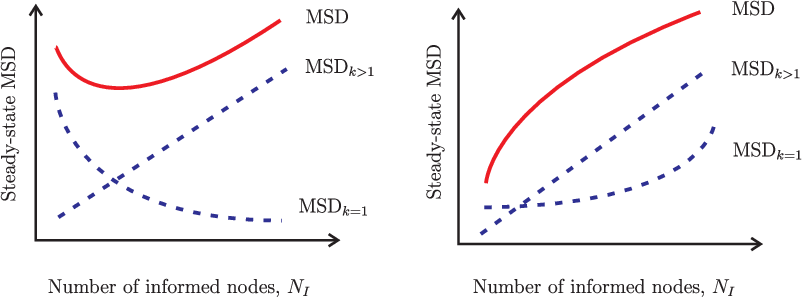
Note that the summations in (122) and (123) are over the set of informed nodes, $\mathcal{N}_{I}$ . Expressions (122) and (123) reveal important information about the behavior of the network. First, the convergence rate in (122) and the network MSD in (123) depend on the network topology only through the node degrees, $\{n_{l}\}$ , and the network degree, $\eta$ . In general, the higher values of $\eta$ are, the slower the convergence rate is (an undesirable effect) and the lower the network MSD is (a desirable effect). Second, as the set of informed nodes, $\mathcal{N}_{I}$ , increases, we observe from (122) that the faster the rate of convergence becomes (a desirable effect). However, as we will illustrate in simulations, the behavior of the terms MSD_k=1 and MSD_k>1 ends up causing the network MSD given by (123) to increase (an undesirable effect) as $\mathcal{N}_{I}$ increases. Figure 4 illustrates the general trend in the behavior of the network MSD and its components, MSD_k=1 and MSD_k>1. Two scenarios are shown in the figure corresponding to the case whether the added informed nodes satisfy (105) or not. The figure shows that depending on condition (105), the curve for MSD_k=1 can increase or decrease with $N_{I}$ . Nevertheless, the overall network MSD generally increases (i.e., becomes worse) with increasing $N_{I}$ . These facts reveal an important trade-off between the convergence rate and the network MSD in relation to the proportion of informed nodes. We summarize the behavior of the ATC network in Table I and show how the rate of convergence and the MSD respond when the parameters $\{\eta,N_{I},\text{Tr}(R_{u})\}$ increase. We remark that slower convergence rate and worse estimation correspond to increasing values of $r$ and MSD (an undesirable effect).

TABLE I: Behavior of the ATC Network in response to increases in any of the parameters

\{\eta,N_{I},{\rm{Tr}}(R_{u})\}

	convergence rate $r$ (122)	MSD (123)	MSD_k=1 (103)	MSD_k>1 (121)
$N_{I}\uparrow$	faster	worse in general	may be better or worse (see (105))	worse
$\eta\uparrow$	slower	better	better	better
$\text{Tr}(R_{u})\uparrow$	faster	worse	independent of $\text{Tr}(R_{u})$	worse

For a proper evaluation of how the proportion of informed nodes influences network behavior, we shall adjust the step-size parameter such that the convergence rate remains fixed as the set of informed nodes is enlarged and then compare the resulting network MSDs. To do so, we set the step-size to the following normalized value:

\mu=\frac{\mu_{0}}{\sum_{l\in\mathcal{N}_{I}}n_{l}}

(124)

for some $\mu_{0}>0$ . Note that this choice normalizes $\mu_{0}$ by the sum of the degrees of the informed nodes. In this way, the convergence rate given by (122) becomes

r\approx\left(1-\frac{\mu_{0}\lambda_{M}(R_{u})}{N\eta}\right)^{2}

(125)

which is independent of the set of informed nodes. Moreover, the network MSD in (123) becomes

\text{MSD}\approx\frac{M\mu_{0}}{2N\eta}\cdot\frac{\sum_{l\in\mathcal{N}_{I}}\sigma^{2}_{v,l}n^{2}_{l}}{\left(\sum_{l\in\mathcal{N}_{I}}n_{l}\right)^{2}}+\frac{\mu_{0}^{2}\text{Tr}(R_{u})}{N\eta}\cdot h\left(\frac{2}{\sqrt{\eta}}\right)\cdot\frac{\sum_{l\in\mathcal{N}_{I}}\sigma^{2}_{v,l}n_{l}}{\left(\sum_{l\in\mathcal{N}_{I}}n_{l}\right)^{2}}

(126)

Using the same argument we used before in (104), if we increase the number of informed nodes by one, the first term in (126) (namely, MSD_k=1) will increase if the degree of the added node satisfies:

\displaystyle n_{N_{I}+1}

\displaystyle\geq\underbrace{2\left[\frac{\sigma^{2}_{v,N_{I}+1}\left(\sum_{l\in\mathcal{N}_{I}}n_{l}\right)^{2}}{\sum_{l\in\mathcal{N}_{I}}\sigma^{2}_{v,l}n^{2}_{l}}-1\right]^{-1}}_{c_{1}}\sum_{l\in\mathcal{N}_{I}}n_{l}

(127)

and the second term in (126) (namely, MSD_k>1) will increase if the degree of the added node satisfies:

\displaystyle n_{N_{I}+1}

\displaystyle\leq\underbrace{\left(\frac{\sigma^{2}_{v,N_{I}+1}\sum_{l\in\mathcal{N}_{I}}n_{l}}{\sum_{l\in\mathcal{N}_{I}}\sigma^{2}_{v,l}n_{l}}-2\right)}_{c_{2}}\sum_{l\in\mathcal{N}_{I}}n_{l}

(128)

In the following, we show that there exist conditions under which both requirements (127) and (128) are satisfied. That is, when this happens and interestingly, the network MSD ends up increasing (an undesirable effect) when we add one more informed node in the network. In the first example, we assume that the degrees of all nodes are the same, i.e., set $n_{l}=n$ for all $l$ . Then, $c_{1}$ and $c_{2}$ in (127)-(128) become

\displaystyle c_{1}=2(N_{I}\beta-1)^{-1},\quad c_{2}=\beta-2

(129)

where

\beta=\frac{\sigma^{2}_{v,N_{I}+1}}{\sum_{l\in\mathcal{N}_{I}}\sigma^{2}_{v,l}/N_{I}}

(130)

It can be verified that if

\beta\geq 2+\frac{1}{N_{I}}

(131)

(or, if the noise variance at the added node is large enough), both (127) and (128) are satisfied and then the MSD will increase (i.e., become worse). A second example is obtained by setting the noise variances to a constant level, i.e., $\sigma^{2}_{v,l}=\sigma^{2}_{v}$ for all $l$ . Then, $c_{1}$ and $c_{2}$ in (127)-(128) become

\displaystyle c_{1}=2\left[\frac{\left(\sum_{l\in\mathcal{N}_{I}}n_{l}\right)^{2}}{\sum_{l\in\mathcal{N}_{I}}n^{2}_{l}}-1\right]^{-1},\quad c_{2}=-1

(132)

In this case, the second term in (126) always decreases, whereas the first term in (126) will increase if the degree of the added informed node is high enough. However, as the number of informed nodes increases, the step-size in (124) will become smaller and the first term in (126) becomes dominant. As a result, the network MSD worsens if (127) is satisfied, i.e., when the added node has large degree. These results suggest that it is beneficial to let few highly noisy or highly connected nodes remain uninformed and participate only in the consultation step (5b).

VI Simulation Results

We consider networks with 200 nodes. The weight vector, $w^{\circ}$ , is a randomly generated $5\times 1$ vector (i.e., $M=5$ ). The regressor covariance matrix $R_{u}$ is a diagonal matrix with each diagonal entry uniformly generated from $[0.8,1.8]$ , and noise variances are set to $\sigma^{2}_{v,k}=0.01$ for all $k$ . The step-size for informed nodes is set to $\mu=0.01$ . Without loss of generality, we assume that the nodes are indexed in decreasing order of degree, i.e., $n_{1}\geq n_{2}\geq\cdots\geq n_{N}$ .

We first verify theoretical expressions (33) and (34) for the network MSD and convergence rate. Figure 5 shows the MSD over time for two network models with parameters $p=0.02$ , $m=2$ , and $N_{0}=10$ . For each network model, we consider two cases: 200 or 50 (randomly selected) informed nodes. We observe that when the number of informed nodes decreases, the convergence rate increases, as expected, but interestingly, the MSD decreases. The theoretical results are also depicted in Fig. 5. The MSD decays at rate $r$ in (34) during the transient stage. When the MSD is lower than the steady-state MSD value from (33), the MSD stays constant at (33). We observe that the theoretical results match well with simulations. The theoretical results (33) and (34) will be used to verify the effectiveness of the approximate expressions (122) and (123).

We examine the effect of the proportion and distribution of informed nodes on the convergence rate and MSD of the network. We increase the number of informed nodes from the node with the highest degree, i.e., from node 1 to node $N$ . The convergence rate and MSD are shown in Fig. 6. For each model, we consider two possible values of parameters: $p=0.02$ and $0.075$ in the Erdos-Renyi model and the $m=2$ and $8$ in the scale-free model. Simulation results are averaged over $30$ experiments. Note from (48) and (50) that the two models have similar network degree. As expected, the convergence rates decrease when we add more informed nodes and expression (122) matches well with expression (34). In addition, the convergence rates in the scale-free model are lower in the beginning because there are some nodes with very high degrees.

TABLE II: Network degree and

|\lambda_{2}(A)|

for two network models

	Erdos-Renyi ( $p$ )		Scale-free ( $m$ )
Parameter ( $p$ or $m$ )	0.02	0.075	2	8
$\eta$	5.13	15.83	4.93	16.33
$\|\lambda_{2}(A)\|$	0.883	0.503	0.900	0.495

Interesting patterns are seen in the MSD behavior. We show $\text{MSD}_{k=1}$ from (103) and $\text{MSD}_{k>1}$ from (115) in Fig. 7. We observe from Fig. 7 that $\text{MSD}_{k=1}$ decreases, whereas $\text{MSD}_{k>1}$ increases with $N_{I}$ . If two network models have similar degree, the scale-free model will have higher values of $\text{MSD}_{k=1}$ and $\text{MSD}_{k>1}$ than the Erdos-Renyi model, and therefore higher values of MSD. This is because the scale-free model has higher values of $n_{l}$ . Since $\text{MSD}_{k=1}$ decreases and $\text{MSD}_{k>1}$ increases, the resulting MSD in (123) can either increase or decrease. The curve of MSD depends on the values of $\text{MSD}_{k=1}$ and $\text{MSD}_{k>1}$ . We observe from Fig. 6 that in most cases, the MSD decreases when $N_{I}$ is small, and then increases with $N_{I}$ . As in the case of a stand-alone adaptive filter, there exists a trade-off between the convergence rate and the MSD. Interestingly, for the scale-free model with higher values of $m$ , we see from Fig. 6 that the MSD decreases with $N_{I}$ . We also see that the approximation for the MSD in (123) matches well with expression (33).

expression () becomes

\text{MSD}\approx\frac{M\mu\sigma^{2}_{v}}{2}\cdot\frac{\sum_{l=1}^{N}n^{2}_{l}}{\left(\sum_{l=1}^{N}n_{l}\right)^{2}}+\mu^{2}\text{Tr}(R_{u})\sigma^{2}_{v}\cdot h\left(\frac{2}{\sqrt{\eta}}\right)

(133)

From the Cauchy-Schwarz inequality and for a fixed value of $\eta$ , we know that

\left(\sum_{l=1}^{N}n_{l}\right)^{2}\leq N\cdot\sum_{l=1}^{N}n^{2}_{l}

(134)

with equality if, and only if, $n_{l}=\eta$ for all $l$ , i.e., all nodes have the same degree. Then, we obtain a lower bound for the MSD:

\text{MSD}\geq\frac{M\mu\sigma^{2}_{v}}{2N}+\mu^{2}\text{Tr}(R_{u})\sigma^{2}_{v}\cdot h\left(\frac{2}{\sqrt{\eta}}\right)

(135)

Since the nodes in the Erdos-Renyi model have similar degree, it will achieve lower MSD than the scale-free model if all nodes are informed.

VI-A MSD with Fixed Convergence Rate

We vary the value of step-size as in (124) with $\mu_{0}=0.1$ and show the network MSD over the number of informed nodes in Fig. 8. To show the MSD possibly increases with $N_{I}$ , we reverse the order in adding informed nodes, i.e., from node $N$ to node 1. It is interesting to note that for the scale-free model, the MSD increases when the number of informed nodes is large. This is because in the scale-free model, there are few nodes connected to most nodes in the network and condition (127) is satisfied. The results suggest that in the scale-free model, we should let few highly connected nodes remain uninformed and perform only the consultation step (5b).

VII Concluding Remarks

In this paper, we derived useful expressions for the convergence rate and mean-square performance of adaptive networks. The analysis examines analytically how the convergence rate and mean-square performance of the network vary with the degrees of the nodes, with the network degree, and with the proportion of informed nodes. The results reveal interesting and surprising patterns of behavior. The analysis shows that there exists a trade-off between convergence rate and mean-square performance in terms of the proportion of informed nodes. It is not always the case that increasing the proportion of informed nodes is beneficial.

References

[1] S. Y. Tu and A. H. Sayed, “On the effects of topology and node distribution on learning over complex adaptive networks,” Proc. Asilomar Conference on Signals, Systems, and Computers, Pacific Grove, CA, Nov. 2011.
[2] C. G. Lopes and A. H. Sayed, “Diffusion least-mean squares over adaptive networks: Formulation and performance analysis,” IEEE Trans. on Signal Processing, vol. 56, no. 7, pp. 3122–3136, Jul. 2008.
[3] F. S. Cattivelli and A. H. Sayed, “Diffusion LMS strategies for distributed estimation,” IEEE Trans. on Signal Processing, vol. 58, no. 3, pp. 1035–1048, Mar. 2010.
[4] S. Camazine, J. L. Deneubourg, N. R. Franks, J. Sneyd, G. Theraulaz, and E. Bonabeau, Self-Organization in Biological Systems. Princeton University Press, 2003.
[5] I. D. Couzin, “Collective cognition in animal groups,” Trends in Cognitive Sciences, vol. 13, pp. 36–43, Jan. 2009.
[6] S. Y. Tu and A. H. Sayed, “Mobile adaptive networks,” IEEE J. Selected Topics on Signal Processing, vol. 5, no. 4, pp. 649–664, Aug. 2011.
[7] F. Cattivelli and A. H. Sayed, “Modeling bird flight formations using diffusion adaptation,” IEEE Trans. on Signal Processing, vol. 59, no. 5, pp. 2038–2051, May 2011.
[8] J. Arenas-Garcia, V. Gomez-Verdejo, and A. R. Figueiras-Vidal, “New algorithms for improved adaptive convex combination of LMS transversal filters,” IEEE Trans. on Instrumentation and Measurement, vol. 54, no. 6, pp. 2239–2249, Dec. 2005.
[9] J. B. Predd, S. B. Kulkarni, and H. V. Poor, “Distributed learning in wireless sensor networks,” IEEE Signal Processing Magazine, vol. 23, no. 4, pp. 56–69, Jul. 2006.
[10] S. Barbarossa and G. Scutari, “Bio-inspired sensor network design,” IEEE Signal Processing Magazine, vol. 24, no. 3, pp. 26–35, May 2007.
[11] T. C. Aysal, M. E. Yildiz, A. D. Sarwate, and A. Scaglione, “Broadcast gossip algorithms for consensus,” IEEE Trans. on Signal Processing, vol. 57, no. 7, pp. 2748–2761, July 2009.
[12] N. Takahashi and I. Yamada, “Link probability control for probabilistic diffusion least-mean squares over resource-constrained networks,” Proc. IEEE ICASSP, pp. 3518–3521, Dallas, TX, Mar. 2010.
[13] U. A. Khan, S. Kar, and J. M. F. Moura, “Higher dimensional consensus: Learning in large-scale networks,” IEEE Trans. on Signal Processing, vol. 58, no. 5, pp. 2836–2849, May 2010.
[14] R. Candido, M. T. M. Silva, and V. H. Nascimento, “Transient and steady-state analysis of the affine combination of two adaptive filters,” IEEE Trans. on Signal Processing, vol. 58, no. 8, pp. 4064–4078, Aug. 2010.
[15] Y. Xia, L. Li, J. Cao, M. Golz, and D. P. Mandic, “A collaborative filtering approach for quasi-brain-death EEG analysis,” Proc. IEEE ICASSP, pp. 645–648, Prague, Czech Republic, May 2011.
[16] S. S. Kozat and A. T. Erdogan, “Competitive linear estimation under model uncertainties,” IEEE Trans. on Signal Processing, vol. 58, no. 4, pp. 2388–2393, Apr. 2010.
[17] S. Sardellitti, M. Giona, and S. Barbarossa, “Fast distributed average consensus algorithms based on advection-diffusion processes,” IEEE Trans. on Signal Processing, vol. 58, no. 2, pp. 826–842, Feb. 2010.
[18] S. Kar and J. M. F. Moura, “Convergence rate analysis of distributed gossip (linear parameter) estimation: Fundamental limits and tradeoffs,” IEEE J. Selected Topics in Signal Processing, vol. 5, no. 5, pp. 674–690, Aug. 2011.
[19] Y. Hu and A. Ribeiro, “Adaptive distributed algorithms for optimal random access channels,” IEEE Trans. Wireless Commun., vol. 10, no. 8, pp. 2703–2715, Aug. 2011.
[20] S. Theodoridis, K. Slavakis, and I. Yamada, “Adaptive learning in a world of projections: A unifying framework for linear and nonlinear classification and regression tasks,” IEEE Signal Processing Magazine, vol. 28, no. 1, pp. 97–123, Jan. 2011.
[21] P. D. Lorenzo and S. Barbarossa, “A bio-inspired swarming algorithm for decentralized access in cognitive radio,” IEEE Trans. on Signal Processing, vol. 59, no. 12, pp. 6160–6174, Dec. 2011.
[22] A. Avitabile, R. A. Morse, and R. Boch, “Swarming honey bees guided by pheromones,” Ann. Entomol. Soc. Am., vol. 68, pp. 1079–1082, 1975.
[23] T. D. Seeley, R. A. Morse, and P. K. Visscher, “The natural history of the flight of honey bee swarms,” Psyche, vol. 86, pp. 103–114, 1979.
[24] S. G. Reebs, “Can a minority of informed leaders determine the foraging movements of a fish shoal?” Anim. Behav., vol. 59, pp. 403–409, 2000.
[25] M. E. J. Newman, D. J. Watts, and A. L. Barabasi, The Structure and Dynamics of Networks. Princeton University Press, 2006.
[26] J. Surowiecki, The Wisdom of Crowds. Anchor Books, 2005.
[27] A. H. Sayed, Adaptive Filters. NJ. Wiley, 2008.
[28] J. Chen and A. H. Sayed, “Diffusion adaptation strategies for distributed optimization and learning over networks,” arXiv:1111.0034, Oct. 2011.
[29] F. S. Cattivelli and A. H. Sayed, “Diffusion strategies for distributed Kalman filtering and smoothing,” IEEE Trans. on Automatic Control, vol. 55, no. 9, pp. 2069–2084, Sep. 2010.
[30] S. Y. Tu and A. H. Sayed, “Diffusion networks outperform consensus networks,” IEEE SSP, Ann Arbor, MI, Aug. 2012 (submitted for publication).
[31] T. Y. Al-Naffouri and A. H. Sayed, “Transient analysis of data-normalized adaptive filters,” IEEE Trans. on Signal Processing, vol. 51, no. 3, pp. 639–652, Mar. 2003.
[32] R. Horn and C. R. Johnson, Matrix Analysis. Cambridge University Press, 1985.
[33] P. Erdos and A. Renyi, “On the evolution of random graphs,” Magyar Tud. Akad. Mat. Kutato Int. Kozl., vol. 5, pp. 17–61, 1960.
[34] A. L. Barabasi and E. Bonabeau, “Scale-free networks,” Scientific American, vol. 288, pp. 50–59, 2003.
[35] A. L. Barabasi and R. Albert, “Emergence of scaling in random networks,” Science, vol. 286, pp. 509–512, 1999.
[36] F. Chung, L. Li, and V. Vu, “Spectra of random graphs with given expected degrees,” Proc. National Academy of Sciences, vol. 100, no. 11, pp. 6313–6318, 2003.
[37] I. J. Farkas, I. Derenyi, A. L. Barabasi, and T. Vicsek, “Spectra of real-world graphs: Beyond the semicircle law,” Phys. Rev. E, vol. 64, no. 026704, 2001.
[38] K. I. Goh, B. Kahng, and D. Kim, “Spectra and eigenvectors of scale-free networks,” Phys. Rev. E, vol. 64, no. 051903, 2001.
[39] S. N. Dorogovtsev, A. V. Goltsev, J. F. F. Mendes, and A. N. Samukhin, “Random networks: Eigenvalue spectra,” Physica A, vol. 338, pp. 76–83, 2004.

$\displaystyle\mathcal{B}\cdot r^{b}_{k,m}$	$\displaystyle=\sum_{l=1}^{N}\lambda_{l}(A)\cdot(r_{l}\otimes I_{M})\left[s^{}_{l,1:N_{I}}r_{k,1:N_{I}}\otimes(1-\mu R_{u})z_{m}+s^{}_{l,N_{I}+1:N}r_{k,N_{I}+1:N}\otimes z_{m}\right]$
	$\displaystyle=\sum_{l=1}^{N}\lambda_{l}(A)\cdot\left[\left(1-\mu\lambda_{m}(R_{u})\right)s^{}_{l,1:N_{I}}r_{k,1:N_{I}}+s^{}_{l,N_{I}+1:N}r_{k,N_{I}+1:N}\right](r_{l}\otimes I_{M})(1\otimes z_{m})$
	$\displaystyle=\sum_{l=1}^{N}\lambda_{l}(A)\cdot\left[s^{}_{l}r_{k}-\mu\lambda_{m}(R_{u})\cdot s^{}_{l,1:N_{I}}r_{k,1:N_{I}}\right]\cdot(r_{l}\otimes z_{m})$
	$\displaystyle\begin{aligned} =\lambda_{k}(A)\cdot\left[1-\mu\lambda_{m}(R_{u})\cdot s^{}_{k,1:N_{I}}r_{k,1:N_{I}}\right]\cdot(r_{k}\otimes z_{m})\\ \phantom{==}-\mu\lambda_{m}(R_{u})\sum_{l\neq k}\lambda_{l}(A)\cdot s^{}_{l,1:N_{I}}r_{k,1:N_{I}}\cdot(r_{l}\otimes z_{m})\end{aligned}$	(69)

$\displaystyle s^{b*}_{k,m}\mathcal{Z}\Omega^{-1/2}$	$\displaystyle=\sum_{l=1}^{N}\lambda_{l}(A)\cdot s^{b}_{k,m}(r_{l}\otimes I_{M})\cdot\begin{bmatrix}s^{}_{l,1:N_{I}}\otimes\mu R_{u}&s^{*}_{l,N_{I}+1:N}\otimes 0_{M}\end{bmatrix}\Omega^{-1/2}$	(83)
	$\displaystyle\approx\frac{\lambda_{k}(A)}{\lambda_{k,m}(\mathcal{B})}\cdot\lambda_{k,m}(\mathcal{B})\cdot(1\otimes z^{}_{m})\begin{bmatrix}s^{}_{k,1:N_{I}}\Sigma^{1/2}_{v,1:N_{I}}\otimes\mu R^{1/2}_{u}&0_{1\times(N-N_{I})M}\end{bmatrix}$
	$\displaystyle=\lambda_{k}(A)\cdot\begin{bmatrix}s^{}_{k,1:N_{I}}\Sigma^{1/2}_{v,1:N_{I}}\otimes\mu\lambda^{1/2}_{m}(R_{u})z^{}_{m}&0_{1\times(N-N_{I})M}\end{bmatrix}$

On the Influence of Informed Agents on Learning and Adaptation over Networks

Abstract

Index Terms:

I Introduction

II Diffusion Adaptation Strategy

III Network Mean-Square Performance

III-A Mean Stability

Theorem 1 (Mean stability).

Proof.

III-B Mean-Square Stability

Theorem 2 (Mean-square stability).

Proof.

III-C Mean-Square Performance

III-D Convergence Rate

Assumption 1.

Lemma 1 (Faster convergence rate).

Proof.

Lemma 2 (Bound on convergence rate).

Proof.

IV Two Network Topology Models

IV-A Erdos-Renyi Model

IV-B Scale-Free Model

V Effect of Topology and Node Distribution

V-A Eigen-structure of ℬ\mathcal{B}

Lemma 3 (Diagonalization of uniform combination matrix).

Proof.

Remark 1.

Lemma 4 (Eigen-structure of ℬ\mathcal{B}).

Proof.

V-B Simplifying the MSD Expression (33)

Theorem 3 (Network MSD).

V-C MSD Expression for the Uniform Combination Matrix from (55)

C.1) Eigenvalues of AA

Theorem 4 (Eigenvalue distribution of AA).

Proof.

C.2) MSD Expression for k=1k=1

C.3) MSD Expression for k>1k>1

Lemma 5.

Proof.

V-D Convergence Rate Expression

V-E Behavior of the ATC Network

Theorem 5 (Network MSD under uniform combination weights).

VI Simulation Results

VI-A MSD with Fixed Convergence Rate

VII Concluding Remarks

References

V-A Eigen-structure of $\mathcal{B}$

Lemma 4 (Eigen-structure of $\mathcal{B}$ ).

C.1) Eigenvalues of $A$

Theorem 4 (Eigenvalue distribution of $A$ ).

C.2) MSD Expression for $k=1$

C.3) MSD Expression for $k>1$