A Turing Machine Resisting Isolated Bursts Of Faults

Ilir Çapuni Affiliation: Boston University Affiliation: Department Of Computer Science Peter Gács Affiliation: 111 Cummington str, Boston MA Affiliation: {ilir, gacs}@cs.bu.edu

Abstract

We consider computations of a Turing machine under noise that causes consecutive violations of the machine’s transition function. Given a constant upper bound $\beta$ on the size of bursts of faults, we construct a Turing machine $M(\beta)$ subject to faults that can simulate any fault-free machine under the condition that bursts are not closer to each other than $V$ for an appropriate $V=O(\beta^{2})$ .

1 Introduction

1.1 The problem

Little is known about the behavior and the power of Turing machines when their operation is subjected to noise that can change arbitrarily the state and the content of the cell where the head is positioned. The main open question, under every noise model, is whether a machine subject to it can perform arbitrary computations reliably.

Here, we construct a Turing machine that—with a slowdown by a multiplicative constant—can simulate any other Turing machine even if the simulator is subjected to constant size bursts of faults separated by a certain minimum number of steps from each other.

The problem of constructing fault-proof machines from components that can fail was first considered by von Neumann in [11], who addressed the problem in the Boolean circuits model. New advances along this path were made in [8, 9]. The question has been considered in uniform models of computation as well. A simple rule for two-dimensional cellular automata that keeps one bit forever even though each cell can fail with some small probability was given in [10]. A 3-dimensional reliably computing cellular automaton using Toom’s rule was constructed in [5]. Alas, all simple one-dimensional cellular automata appear to be “ergodic” (forgetting everything about their initial configuration in time independent of the size). The first, complex, nonergodic cellular automaton was constructed in [3], and improved upon in [4]. It supports a hierarchical organization, based on an idea given in [6]. Cells are organized in units that perform fault-tolerant simulation of another automaton (of the same kind). The latter simulates even more reliably a third automaton of a similar kind, and so on.

The question of reliable computation with Turing machines (where arbitrarily large bursts may occur with correspondingly small probability) is raised in [4]. As in the case of one-dimensional cellular automata, no simple solution to this problem appears to exist. The present paper’s machine is intended as a building block towards the eventual (hierarchical) construction of such a machine. This follows the paradigm of the proof in [3], where each member of the hierarchy of simulations is a similar building block, coping with distant bursts. To the best of our knowledge, this is the first construction of a sequential machine, reliable in a similar sense.

The title of [1] suggests some connection, but that paper’s interest is completely different: it examines the expressional ability, in terms of the arithmetical hierarchy, of Turing machines whose storage tapes are exposed to stochastic noise that tends to zero.

1.2 Simulating cellular automata

It is natural to try to derive fault-tolerant Turing machines from the existing results on fault-tolerant cellular automata. Cannot one simply define a Turing machine that simulates a fault-tolerant cellular automaton? In some sense, the answer is yes. Suppose that we know in advance the memory requirement $m=S(x)$ of a computation on a fault-tolerant cellular automaton $M$ , on input $x$ . The we can define a special Turing machine $T(m)$ , working on a circular tape of size $m$ , with the head moving always in the right direction (in other words, the “oblivious” property is hardwired), where each pass of $T$ over the tape simulates one step of $M$ . This machine will clearly have the same fault-tolerance properties that $M$ has.

The circular Turing machine has a strong fault-tolerant behavior (with a sophisticated transition rule, coming from the cellular automaton it simulates). Our efforts on fault-tolerant Turing machines can be seen as just aiming to remove the limitation of circular tape (input size-dependent hardware).

In view of the above, it would be sufficient to define fault-tolerant sweeping behavior on a regular tape (once the head can change direction, the sweeping movement can be disturbed by faults): the rest can be done by simulating a cellular automaton. We were, however, not able to do this without recreating the hierarchical constructions used in cellular automata—with all the necessary changes for Turing machines.

1.3 Turing machines

Our contribution uses one of the standard definitions of a Turing machine, with the exception of no halting state.

Definition 1.1.

A Turing machine $M$ is defined by a tuple

\displaystyle(\Gamma,\Sigma,\delta,q_{\textit{start}},F).

Here, $\Gamma$ is a finite set of states, $\Sigma$ is a finite alphabet used in cells of the tape, and

\displaystyle\delta:\Sigma\times\Gamma\to\Sigma\times\Gamma\times\{-1,0,+1\}

is a transition function. The tape alphabet $\Sigma$ contains at least the distinguished symbols $\text{\textvisiblespace},0,1$ where ␣ is called the blank symbol. The distinguished state $q_{\textit{start}}$ is called the starting state. The set $F$ of final states has the property that whenever $M$ enters a state in $F$ , it can only continue from there to another state in $F$ , without changing the tape.

A configuration is a tuple

\displaystyle(q,h,x),

where $q\in\Gamma$ , $h\in\mathbb{Z}$ and $x\in\Sigma^{\mathbb{Z}}$ . Here, $x[p]$ is the content of the tape cell at position $p$ . The tape is blank at all but finitely many positions. The work of the machine can be described as a sequence of configurations $C_{0},C_{1},C_{2},\dots$ , where $C_{t}$ is the configuration at time $t$ . If $C=(q,h,x)$ is a configuration then we will write

\displaystyle C.\textit{state}=q,\quad C.\textit{pos}=h,\quad C.\textit{tape}=x.

Here, $x$ is also called the tape configuration. ∎

Though the tape alphabet may contain non-binary symbols, we will restrict input and output to binary.

Definition 1.2.

For an arbitrary binary string $x$ , let

\displaystyle M(x,t)

(1.1)

denote the configuration at time $t$ , when started from a binary input string $x$ written on the tape starting from position 0, with head position 0 and the starting state. Thus, the symbol at tape position $p$ at time $t$ can be written

\displaystyle M(x,t).\textit{tape}[p].

The transition function $\delta$ tells us how to compute the next configuration from the present one. When the machine is in a state $q$ , at tape position $h$ , and observes tape cell with content $a$ , then denoting

\displaystyle(a^{\prime},q^{\prime},j)=\delta(a,q),

it will change the state to $q^{\prime}$ , change the tape cell content to $a^{\prime}$ and move to tape position to $h+j$ . For $q\in F$ we have $a^{\prime}=a$ , $q^{\prime}\in F$ . ∎

We say that a fault occurs at time $t$ if the output $(a^{\prime},q^{\prime},j)$ of the transition function at this time is replaced with some other value (which is then used to compute the next configuration). For the sake of a clean definition of simulations, we will be more formal in defining fault-free histories.

Definition 1.3 (Trajectory).

Let

\displaystyle\mathrm{Configs}_{M}

denote the set of all possible configurations of a Turing machine $M$ . Consider a sequence $\eta=(\eta(0),\eta(1),\dots)$ of configurations of $M=(\Gamma,\Sigma,\delta)$ with $\eta(t)=(q(t),h(t),x(t))$ . This sequence will be called a history of $M$ if the following conditions hold:

•

$q(0)=q_{\textit{start}}$ .
•

$x(t+1)[n]=x(t)[n]$ for all $n\neq h(t)$ .
•

$h(t+1)-h(t)\in\{-1,0,1\}$ .

Let

\displaystyle\mathrm{Histories}_{M}

denote the set of all possible histories of $M$ . A history $\eta$ with $\eta(t)=(q(t),h(t),x(t))$ of $M$ is called a trajectory of $M$ if for all $t$ we have

(x(t+1)[h(t)],q(t+1),h(t+1)-h(t))=\delta(x(t),q(t)).

(1.2)

We say that a history has a fault at time $t$ if (1.2) is violated at time $t$ . (Thus, if a history has any one fault, it is not a trajectory.) A burst of faults of a history is a sequence of times containing some faults. ∎

With the earlier notation (1.1), if $x\in\Sigma^{*}$ is a string of nonblank tape symbols, then the history defined by

\displaystyle\eta(t)=M(x,t)

for all $t$ is a trajectory in which $\eta(0)$ is a starting tape configuration obtained by surrounding $x$ with blanks.

1.4 Codes

To define simulation of a noise-free machine $M_{2}$ by a noisy machine $M_{1}$ , we need to specify the correspondence between configurations of these two machines. After a burst, the state of the machine—as well as the state of cells where the head was during the burst, could have been changed in an arbitrary way. To proceed with the simulation, the simulating machine must recover the information lost. Redundant storage will help. In Section 3, we will specify how one step of $M_{2}$ is simulated by a bounded number of steps of $M_{1}$ .

We formalize redundant storage with the help of codes.

Definition 1.4 (Code).

Let $\Sigma_{1},\Sigma_{2}$ be two finite alphabets. A block code is given by a positive integer $Q$ , an encoding function $\varphi_{*}:\Sigma_{2}\to\Sigma_{1}^{Q}$ and a decoding function $\varphi^{*}:\Sigma_{1}^{Q}\to\Sigma_{2}$ with the property $\varphi^{*}(\varphi_{*}(x))=x$ . ∎

Definition 1.5 (Standard pairing).

For every alphabet $\Sigma$ that we will consider, we assume that there is a standard ordering of its elements: $\Sigma=\{s_{1},\dots,s_{n}\}$ . This gives rise to a code

\displaystyle(\gamma_{*},\gamma^{*}),

where $\gamma_{*}(s_{i})$ is the base 2 notation of the number $i$ , padded from the front to length ${\lceil\log n\rceil}$ . For example, if $\Sigma=\{s_{1},s_{2},s_{3}\}$ then the codewords are $01,10,11$ .

For a (possibly empty) binary string $x=x(1)\dotsm x(n)$ let us introduce the map

x^{o}=x(1)x(1)x(2)x(2)\dotsm x(n)x(n).

If $s$ is a symbol in some alphabet $\Sigma$ then by ${\mathopen{\langle}s\mathclose{\rangle}}$ we will understand $(\gamma_{*}(s))^{o}$ , and call it the standard prefix-free code of $s$ . Similarly,

	$\displaystyle{\mathopen{\langle}s,t\mathclose{\rangle}}$	$\displaystyle={\left((\gamma_{}(s))^{o}\gamma_{}(t)\right)}^{o},$
	$\displaystyle{\mathopen{\langle}s,t,u\mathclose{\rangle}}$	$\displaystyle={\mathopen{\langle}s,{\mathopen{\langle}t,u\mathclose{\rangle}}\mathclose{\rangle}},$

and so on. ∎

We have $|x^{o}|=2|x|+2$ . There are shorter codes with the same prefix-free property,but minimizing the code length is not our concern here.

Definition 1.6 (Error-correcting code).

A block code is $(\beta,t)$ -burst-error-correcting, if for all $x\in\Sigma_{2}$ , $y\in\Sigma_{1}^{Q}$ we have $\varphi^{*}(y)=x$ whenever $y$ differs from $\varphi_{*}(x)$ in at most $t$ intervals of size $\leq\beta$ . ∎

Example 1.7 (Tripling).

Suppose that $Q\geq 3\beta$ is divisible by 3, $\Sigma_{2}=\Sigma_{1}^{Q/3}$ , $\varphi_{*}(x)=xxx$ . Let $\varphi^{*}(y)$ be obtained as follows. If $y=y(1)\dots y(Q)$ , then $x=\varphi^{*}(y)$ is defined as follows: $x(i)=\mathop{\mathrm{maj}}(y(i),y(i+Q/3),y+2Q/3)$ . For all $\beta\leq Q/3$ , this is a $(\beta,1)$ -burst-error-correcting code.

If we repeat 5 times instead of 3, we get a $(\beta,2)$ -burst-error-correcting code (there are also much more efficient such codes than just repetition). ∎

We will also need a more general majority function later on:

Definition 1.8.

Let $x=(x_{1},\dots,x_{n})$ be a sequence of symbols from a finite alphabet $\Sigma=\{a_{1},a_{2},\dots,a_{m}\}$ . For each $j=1,2,\dots,m$ , let $k_{j}$ be the number of occurrences of $a_{j}$ in $x$ , $k_{1}+k_{2}+\dots+k_{m}=n$ . Then,

\displaystyle\mathop{\mathrm{maj}}(x_{1},x_{2},\dots,x_{n})=a_{k},

where $k=\arg\max_{j}{k_{j}}$ . ∎

In the Section 3.5, we will show how to compute a majority of values in a sequence of cells using only one pass over the sequence.

Definition 1.9 (Configuration code).

A configuration code is a pair of functions

\displaystyle\varphi_{*}:\Sigma_{2}^{\mathbb{Z}}\to\Sigma_{1}^{\mathbb{Z}},\quad\varphi^{*}:\Sigma_{1}^{\mathbb{Z}}\to\Sigma_{2}^{\mathbb{Z}}

that encodes infinite strings of $\Sigma_{2}$ into infinite strings of $\Sigma_{1}$ . Each block code $(\varphi_{*},\varphi^{*})$ gives rise to a natural tape configuration code which we will also denote by $(\varphi_{*},\varphi^{*})$ . If $\xi=\dotsm\xi(-1)\xi(0)\xi(1)\dotsm$ is an infinite string of letters of $\Sigma_{2}$ then $\varphi_{*}(x)$ is the string

\displaystyle\dotsm\varphi_{*}(\xi(-1))\varphi_{*}(\xi(0))\varphi_{*}(\xi(1))\dotsm,

while for decoding an infinite configuration $\xi^{\prime}$ we subdivide it first into blocks of size $Q$ (starting with $\xi^{\prime}(0)\dotsm\xi^{\prime}(Q-1)$ ), decode each block separately, and concatenate the results. ∎

1.5 The result

We will define our result in terms of universal Turing machines, operating on binary strings as inputs and outputs.

Definition 1.10 (Computation result).

Assume that a Turing machine $M$ starting on binary $x$ , at some time $t$ arrives at the first time at some final state. Then we look at the longest (possibly empty) binary string to be found starting at position 0 on the tape, and call it the computation result $M(x)$ . ∎

Definition 1.11 (Universal Turing machine).

We say that Turing machine $U$ is universal among Turing machines with binary inputs and outputs, if for every Turing machine $M$ , for all binary strings $x$ , there is a binary string $p_{M}$ such that $M$ reaches a final state on input $x$ if and only if $U$ reaches a final state on input ${\mathopen{\langle}p_{M}\mathclose{\rangle}}x$ , further in this case we have $U({\mathopen{\langle}p_{M}\mathclose{\rangle}}x)=M(x)$ . A universal Turing machine will be called flexible if whenever $U({\mathopen{\langle}p,q\mathclose{\rangle}}x)$ halts, also $U({\mathopen{\langle}p\mathclose{\rangle}}q)$ halts, and $U({\mathopen{\langle}p,q\mathclose{\rangle}}x)=U(U({\mathopen{\langle}p\mathclose{\rangle}}q)x)$ . In other words if a program has the form ${\mathopen{\langle}p,q\mathclose{\rangle}}$ then $U$ first applies as a preprocessing step the program $p$ to $q$ , and then it starts work on the result attached in front of $x$ .

It is well-known that there are flexible universal Turing machines. Let us fix one and call it $U$ .

Consider an arbitrary Turing machine $M$ with state set $\Gamma$ , alphabet $\Sigma$ , and transition function $\delta$ . A binary string $p$ will be called a transition program of $M$ if whenever $\delta(a,q)=(a^{\prime},q^{\prime},j)$ we have

\displaystyle U({\mathopen{\langle}p\mathclose{\rangle}}{\mathopen{\langle}a,q\mathclose{\rangle}})={\mathopen{\langle}a^{\prime},q^{\prime},j\mathclose{\rangle}}.

We will also require that the computation induced by the program makes $O(|p|+|a|+|q|)$ left-right turns, over a length tape $O(|p|+|a|+|q|)$ . ∎

The transition program just provides a way to compute the (local) transition function of $M$ by the universal machine, it does not organize the rest of the simulation.

Remark 1.12.

In the construction provided by the textbooks, the program is generally a string encoding a table for the transition function $\delta$ of the simulated machine $M$ . Other types of program are imaginable: some simple transition functions can have much simpler programs. However, our fixed machine is good enough. Let the fixed program $r$ be such that $U({\mathopen{\langle}r\mathclose{\rangle}}{\mathopen{\langle}x,y\mathclose{\rangle}})={\mathopen{\langle}x\mathclose{\rangle}}{\mathopen{\langle}y\mathclose{\rangle}}$ . If some machine $U^{\prime}$ simulates $M$ via a very simple program $q$ , then $U$ will simulate $M$ via program ${\mathopen{\langle}r,{\mathopen{\langle}p_{U^{\prime}},q\mathclose{\rangle}}\mathclose{\rangle}}$ :

\displaystyle U({\mathopen{\langle}r,{\mathopen{\langle}p_{U^{\prime}},q\mathclose{\rangle}}\mathclose{\rangle}}x)=U({\mathopen{\langle}p_{U^{\prime}}\mathclose{\rangle}}{\mathopen{\langle}q\mathclose{\rangle}}x)=U^{\prime}({\mathopen{\langle}q\mathclose{\rangle}}x)=M(x).

∎

For simplicity, we will consider only computations whose result is a single symbol, at tape position 0:

\displaystyle M(x,t).\textit{tape}[0]

at any time $t$ in which $M(x,t).\textit{state}$ is a final state. This frees us of the problem of having to decode before announcing the final result of the fault-tolerant computation. We will prove:

Theorem 1.13 (Main).

For a given Turing machine $M_{2}$ with transition program $p_{2}$ , and positive integer $\beta$ , following items can be constructed:

•

Integers $Q$ depending linearly on $\beta$ and $p_{2}$ , logarithmically on $|\Sigma_{2}|$ , $|\Gamma_{2}|$ , further $V$ depending quadratically on $Q$ ;
•

A block code $(\varphi_{*},\varphi^{*})$ of blocksize $Q$ ;
•

A machine $M_{1}$ whose number of states and alphabet size depend polynomially on $Q$ , with some function $f$ defined on its alphabet;

such that the following holds.

Suppose that on input $x$ , the fault-free machine $M_{2}$ enters a final state at time $T$ . Assume that $\eta$ is a history of machine $M_{1}$ on starting configuration $\varphi_{*}(x)$ such that bursts of faults have size at most $\beta$ , and are separated by at most $V$ steps from each other. Let $t$ be any time $\geq VT$ such that no fault occurred in the last $V$ steps before and including $t$ , then

\displaystyle f(\eta(t).\textit{tape}[0])=M_{2}(x,T).\textit{tape}[0].

(1.3)

Section 2 specifies the layout of the tape and the structure of the states, and introduces the notion of rules. The parts of the transition function of $M_{1}$ dealing with redundant simulation are defined in Section 3. Section 4 introduces the parts allowing to restore the structure of the simulation after locally garbled by faults. The main theorem is proved in Section 5.

2 Program Structure

2.1 Fields

Each state of the simulating machine $M_{1}$ will be a tuple $q=(q_{1},q_{2},\dots,q_{k})$ , where the individual elements of the tuple will be called fields, and will have symbolic names. For example, we will have fields Info and Drift, and may write $q_{1}$ as $q.\textit{Info}$ or just Info, $q_{2}$ as $q.\textit{Drift}$ or Drift, and so on.

We will call the current direction of the simulated machine $M_{2}$ the drift ( $-1$ for left, 0 for none, and $+1$ for right).

A properly formatted configuration of $M_{1}$ splits the tape into blocks of $Q$ consecutive cells called colonies. One colony of the tape of the simulating machine represents one cell of the simulated machine. The colony that corresponds to the active cell of the simulated machine (that is the cell that the simulated machine is scanning) is called the base colony (later we will give a precise definition of this notion based on the actual history of the work of $M_{1}$ ). Once the drift is known, the union of the base colony with the neighbor colony in the direction of the drift is called the extended base colony (more precisely, see Definition 4.2).

The head will make some global sweeping movements over the extended base colony. We will use term sweep direction. But even while the sweep direction does not change, the head will make frequent short switchbacks (zigzags).

The states of machine $M_{1}$ will have a field called mode. The normal mode corresponds to the states where $M_{1}$ is performing the simulation of $M_{2}$ . The recovery mode tries to correct some perceived fault.

Similarly, each cell of the tape of $M_{1}$ consists of several fields. Some of these have names identical to fields of the state. In describing the transition rule of $M_{1}$ we will write, for example, $q.\textit{Info}$ simply as Info, and for the corresponding field $a.\textit{Info}$ of the observed cell symbol $a$ we will write c.Info. The array of values of the same field of the cells will be called a track. Thus, we will talk about the c.Hold track of the tape, corresponding to the c.Hold field of cells.

2.2 Rules

Instead of writing a single huge transition table, we present the transition function as a set of rules. Each rule consists of some conditional statements, similar to the ones seen in an ordinary program: “if condition then $\dots$ ”, where the condition is testing values of some fields of the state and the observed cell. Even though rules are written like procedures of a program, they describe a single transition. When several consecutive statements are given, then they (almost always) change different fields of the state or cell symbol, so they can be executed simultaneously. Otherwise and in general, even if a field is updated in some previous statement, in all following statements that use this field, its old value is considered.

Rules can call other rules, but these calls will never form a cycle. We will also use some conventions introduced by the C language: namely, $x\leftarrow x+1$ and $x\leftarrow x-1$ are abbreviated to $x\mathord{+}\mathord{+}$ and $x\mathord{-}\mathord{-}$ respectively.

Rules can also have parameters, like $\texttt{Swing\/}(a,b,u,v)$ (see below). Since each rule is called only a constant number of times in the whole program, the parametrized rule can be simply seen as a shorthand.

2.3 List of fields

The basic fields of the state and of cells are listed below, with some hints of their function (this does not replace our later definition of the transition function). We will not repeat every time that each field of a cell has also a possible value $\emptyset$ corresponding to the case when the state is blank.

We recommend to skip this list at first reading, and to return to it just for reference.

1.

Addr ranges from $-Q$ to $2Q-1$ . The values $-Q$ to $-1$ are taken during the left drift, while the values $Q$ to $2Q-1$ during a right drift. During the first sweep of the work period, Addr is reduced modulo $Q$ .
2.

Dir stores the direction of the previous step.
3.

Drift stores the direction of the simulated machine $M_{2}$ . It may have values $\emptyset,-1,0,1$ . The value $\emptyset$ corresponds to the case when the new Drift is still not computed, and will also be the default value (for example in empty cells). The c.Drift field of the cells of the extended colony correspond to Drift in the state.
4.

Sw numbers the sweeps through the colony. The first sweep of a work period has number 1 and is to the right, and this way each right sweep is odd, each left sweep is even. Thus the sweep direction of the head is completely determined by the parity of Sw, unless the head is at a “turning” point. At turning points, Sw is incremented.

Field c.Sw holds the number of the most recent sweep. The simulation consists of a computation phase and a transferring phase, each corresponding to a certain interval of sweep values to be specified below (these intervals depend somewhat on the value Drift).

The triple of fields $(\textit{c.Addr},\textit{c.Sw},\textit{c.Drift})$ will determine the role played by a cell in the colony work period: for notational convenience, we introduce the names

\displaystyle\textit{Core}=(\textit{Addr},\textit{Sw},\textit{Drift}),\quad\textit{c.Core}=(\textit{c.Addr},\textit{c.Sw},\textit{c.Drift}).

(2.1)

6.

The Info and State tracks represent the tape symbols and the state of the simulated machine $M_{2}$ .
7.

The sweep-through is interrupted by switchbacks called zigging, described by a rule $\texttt{Zigzag\/}(d)$ . Here $d$ is the direction of sweep. The process also depends on a fixed parameter

$\displaystyle Z=22\beta,$ (2.2)

and is controlled by the fields ZigDepth and ZigDir of the state.

From now on, we will assume that $Q$ is a multiple of $Z-4\beta$ :

$\displaystyle(Z-4\beta)|Q.$ (2.3)

Every $Z-4\beta$ forward steps are accompanied by $Z$ steps backward and forward, for a total of

$\displaystyle 3Z-4\beta=3(Z-4\beta)+8\beta<4(Z-4\beta)$

steps.

Figure 1: A sweep of a base colony with zigging.
8.

The Mode field takes values in $\{\mathrm{Normal},\mathrm{Recovering}\}$ . In the absence of faults, the state would never leave the normal mode. On noticing any disorder, the state will switch to recovery mode, with the goal of eventually returning to normal mode.

The fields used in recovery mode are all collected as subfields of the field Rec of the state, and the field c.Rec of the cell state. They will be introduced in the definition of the recovery rule.

In particular, when the field

$\displaystyle\textit{c.Rec}.\textit{Core}$ (2.4)

is not $0$ , we will call the cell marked.
9.

Even though we store information with redundancy, faults can disturb the coding and decoding operations and the simulating computation itself. Therefore these procedures will be repeated several times, and their results, serving as candidates of the final values of $(\textit{Info},\textit{Drift},\textit{State})$ , will be stored in the c.Hold track. The different candidates will be stored in the different parts of the c.Hold field, which is actually a small array $\textit{c.Hold}[1]$ , $\textit{c.Hold}[2]$ , $\textit{c.Hold}[3]$ . The subfield $\textit{c.Hold}[i].\textit{Info}$ holds the value of the $i$ -th candidate for the new Info value of the current cell.

Machine $M_{1}$ has no final states: even when the simulated computation ends the simulation continues to defend the end result from faults.

3 The Simulation

One computational step of the machine $M_{2}$ is simulated by many steps of $M_{1}$ that make one unit called the work period.

3.1 Coding

We will frequently make use of the parameter

\displaystyle E=30Z.

(3.1)

For simplicity, let us assume that the set of states $\Gamma_{2}$ , and the alphabet $\Sigma_{2}$ are subsets of the set of binary strings $\{0,1\}^{\ell}$ for some $\ell<Q$ (we can always ignore some states or tape symbols, if we want). We will then use the same code $(\upsilon_{*},\upsilon^{*})$ for both the states of machine $M_{2}$ and its alphabet. Let $(\upsilon_{*},\upsilon^{*})$ be a $(\beta,2)$ -burst-error-correcting code

\displaystyle\upsilon_{*}:\{0,1\}^{\ell}\to\{0,1\}^{Q-2.2E}.

(The length of the code is not $Q$ , only $Q-2.2E$ , since we will leave place the codeword at a distance $1.1E$ from both colony ends.) We could use, for example, the tripling code of Example 1.7. Other codes are also appropriate, but we require that they have some fixed, constant programs $p_{\mathrm{encode}}$ , $p_{\mathrm{decode}}$ on the universal machine $U$ , in the following sense:

\displaystyle\upsilon_{*}(x)=U({\mathopen{\langle}p_{\mathrm{encode}}\mathclose{\rangle}}x),\quad\upsilon^{*}(y)=U({\mathopen{\langle}p_{\mathrm{decode}}\mathclose{\rangle}}y).

Also, these programs must work in quadratic time and linear space on a one-tape Turing machine (as tripling certainly does).

Let $a$ be the tape configuration of $M_{2}$ at time 0, and $s$ the starting state of $M_{2}$ . The initial tape configuration $a^{\prime}=\varphi_{*}(a)$ of $M_{1}$ is defined as follows:

	$\displaystyle a^{\prime}[h\cdot Q+1.1E,\dots,(h+1)Q-1.1E-1].\textit{Info}$	$\displaystyle=\upsilon_{*}(a[h]),$		(3.2)
	$\displaystyle a^{\prime}[1.1E,\dots,Q-1.1E-1].\textit{State}$	$\displaystyle=\upsilon_{*}(s).$		(3.3)

In cells of the base colony and its left neighbor colony, the c.Sw and c.Drift fields are set to $\mathrm{Last}(+1)$ and $1$ respectively, where $\mathrm{Last}(+1)$ denotes the last sweep of a working period for the positive drift (and is defined below in (3.8)). In the right neighbor colony, these values are $\mathrm{Last}(-1)$ and $-1$ respectively. In all other cells, these values are empty.

The head is initially located at the first cell of the base colony. We assume that the Addr fields of each colony are filled properly, that is

\displaystyle a^{\prime}[i].\textit{Addr}=i\bmod Q.

The c.Hold values are empty in each cell.

Machine $M_{1}$ starts in normal mode, $\textit{Drift}=1$ , $\textit{Sw}=1$ . All other fields have also their initial (or empty) values (see Figure 2).

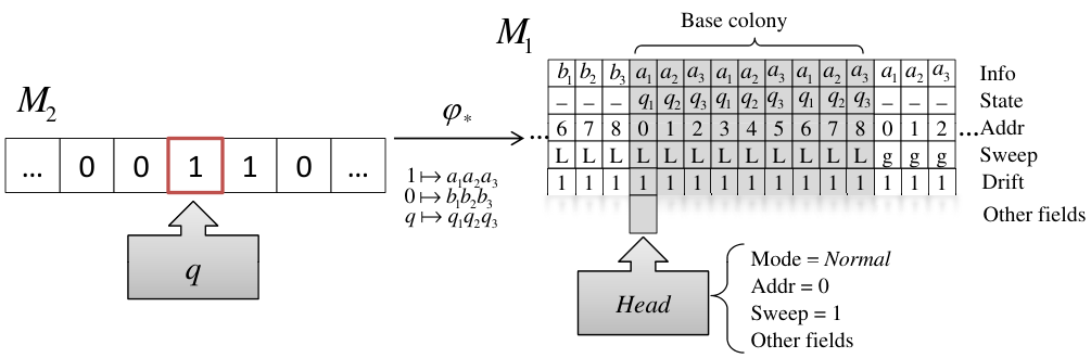
Refer to caption — Figure 2: The initial configuration of machine $M_{2}$ is encoded into the initial configuration of $M_{1}$ , where $L=\mathrm{Last}(1)$ , $g=\mathrm{Last}(-1)$ .

The corresponding block decoding function $\varphi^{*}$ is obtained applying the decoding function $\upsilon^{*}$ to just the c.Info track of $M_{1}$ (actually to just the part between addresses $1.1E$ and $Q-1.1E$ of each colony) to obtain the tape of the simulated machine $M_{2}$ , and to just the c.State track of the base colony to obtain its state.

This definition of decoding will be refined for configurations different from the initial one, since the location of the base colony must also be found using decoding.

3.2 Sweep counter and direction

The global sweeping movement of the head will be controlled by the parametrized rule

\displaystyle\texttt{Swing\/}(a,b,u,v).

This rule makes the head swing between two extreme points $a,b$ , while the counter Sw increases from value $u$ to value $v$ . The Sw value is incremented at the “turns” $a,b$ (and is also recorded on the track c.Sw).

The sweep direction $\delta$ of the simulating head is derived from Sw, Addr and the current value Dir in the following way. On arrival of the head to an endpoint (that is when $\textit{Dir}\neq 0$ and $\textit{Addr}\in\{a,b\}$ ), the values Sw and c.Sw are incremented and Dir is set to 0. In all other cases, the sweep direction is determined by the formula

\displaystyle\mathrm{dir}(s)=(-1)^{s+1}.

(3.4)

Let

\delta=\begin{cases}0&\text{ if $\textit{Addr}\in\{a,b\}$ and $\textit{Dir}\neq 0$},\\ \mathrm{dir}(\textit{Sw})&\text{otherwise}.\end{cases}

(3.5)

As an example of rules, we present the zigging rule in Rule 3.2, which itself uses the rule $\texttt{Move\/}(d)$ . At each non-zigging step, $\textit{Addr}\leftarrow\textit{Addr}+\delta$ .

Rule 3.1

\texttt{Move\/}(d)

\textit{Dir}\leftarrow d

d\in\{-1,0,1\}

\textit{Mode}=\mathrm{Normal}

then

\textit{Addr}\leftarrow\textit{c.Addr}\leftarrow\textit{Addr}+d

else

\textit{Rec}.\textit{Addr}\leftarrow\textit{Rec}.\textit{Addr}+d

Move in direction

d

Rule 3.2

\texttt{Zigzag\/}(d)

d\in\{-1,1\}

is the direction of progress.

\textit{ZigDir}=-1

and ((

\textit{ZigDepth}=0

and

(Z-4\beta)|\textit{Addr}

)

0<\textit{ZigDepth}<Z

) then

\textit{ZigDepth}\mathord{+}\mathord{+}

\textit{ZigDepth}=Z-1

then

\textit{ZigDir}=1

\texttt{Move\/}(-d)

else if

\textit{ZigDir}=1

or (

\textit{ZigDepth}=0

and

(Z-4\beta)\not|\textit{Addr}

) then

\textit{ZigDepth}>0

then

\textit{ZigDepth}\mathord{-}\mathord{-}

else

\textit{ZigDir}\leftarrow-1

\texttt{Move\/}(d)

3.3 The computation phase

The aim of this phase is to obtain new values for c.State, c.Drift and c.Info. It essentially repeats three times the following stages: decoding, applying the transition, encoding. In more detail:

1.
For every $j=1,2,3$ do
1. (a)
  
  Calling by $g$ the string found on the c.State track of the base colony between addresses $1.1E$ and $Q-1.1E$ , decode it into string $\hat{g}=\upsilon^{*}(g)$ (this should be the current state of the simulated machine $M_{2}$ ), and store it on some auxiliary track in the base colony. Do this by simulating the universal machine on some work track, with the program $p_{\mathrm{decode}}$ : $\hat{g}=U({\mathopen{\langle}p_{\mathrm{decode}}\mathclose{\rangle}}g)$ .
  
  Proceed similarly with the string $a$ found on the c.Info track of the base colony, to get $\hat{a}=\upsilon^{*}(a)$ (this should be the observed tape symbol of the simulated machine $M_{2}$ ).
2. (b)
  
  Compute the value
  
  $\displaystyle(a^{\prime},g^{\prime},d)=\delta_{2}(\hat{a},\hat{g})$
  
  similarly, simulating the universal machine $U$ with program $p_{2}$ . The string $p_{2}$ (as well as the constant-size programs $p_{\mathrm{decode}},p_{\mathrm{decode}}$ ) is “hardwired” into the transition function of $M_{1}$ , that is the program we are writing. More precisely, before performing the computation of $U({\mathopen{\langle}p_{2}\mathclose{\rangle}}{\mathopen{\langle}\hat{a},\hat{q}\mathclose{\rangle}})$ of Definition 1.11, machine $M_{1}$ writes the program $p_{2}$ onto some work track: for this, the string $p_{2}$ will be a literal part of the program of $M_{1}$ .
3. (c)
  
  Write the encoded new state $\upsilon_{*}(g^{\prime})$ onto the $\textit{c.Hold}[j].\textit{State}$ track of the base colony between positions $1.1E$ and $Q-1.1E$ .
  
  Similarly, write the encoded new observed cell content $\upsilon_{*}(a^{\prime})$ onto the $\textit{c.Hold}[j].\textit{Info}$ track of the base colony. Write also the first symbol of $a^{\prime}$ into position 0 of the same track (just because the Main Theorem 1.13 expects the result of the whole computation at tape position 0, not $1.1E$ ).
  
  Write $d$ into the $\textit{c.Hold}[j].\textit{Drift}$ field of each cell of the base colony.
2.

Repeat the following twice:

Sweeping through the base colony, at each cell compute the majority of $\textit{c.Hold}[j].\textit{Info}$ , $j=1,2,3$ , and write into the field c.Info. Proceed similarly, and simultaneously, with State and Drift.

It can be arranged—and we assume so—that the total number of sweeps of this phase, and thus the starting sweep number of the next phase,

$\displaystyle\mathrm{TfSt}=O(Q),$ (3.6)

depends only on $Q$ .


(a)		(b)

Figure 3: A work period of the machine

M_{1}

(zigging and many sweeps are not shown, for clarity). In (a) the machine drifts left, while in (b) it drifts right.

3.4 Transfer phase

The aim of this phase, present only if $\textit{Drift}\neq 0$ , is to transfer the new State of $M_{2}$ into the neighbor colony in the direction of $\delta=\textit{Drift}$ (which was computed in the previous phase), and to move there. $\mathrm{TfSw}(\delta)$ is the transfer sweep, the sweep in which we start transferring in direction $\delta$ :

\mathrm{TfSw}(1)=\mathrm{TfSt},\quad\mathrm{TfSw}(-1)=\mathrm{TfSt}+1.

(3.7)

The phase consists of the following actions.

1.

Spread the value $\delta$ found in the cells of the c.Drift track (they should all be the same) onto the neighbor colony in direction $\delta$ .
2.

For $i=1,2,3$ :

Copy the content of c.State track of the base colony to the $\textit{c.Hold}[i].\textit{State}$ track of the neighbor colony.
3.

Assign the field majority: $\textit{c.State}\leftarrow\mathop{\mathrm{maj}}(\textit{c.Hold}[1\dots 3].\textit{State})$ in all cells of the neighbor colony. This part ends with a sweep value $\mathrm{TransferLast}$ depending only on the program $p_{2}$ .
4.

If $\textit{Drift}=1$ , then move right to cell $Q$ (else stay where you are).

The last sweep number of the work period is

\displaystyle\mathrm{Last}(\delta)=\mathrm{TransferLast}+\max(0,\delta).

(3.8)

The work period in case of both non-zero drift values is illustrated in Figure 3.

3.5 Interval plurality

We give an algorithm that computes the plurality of some field c.F over some interval, that is, the value that appears the most, but at least $1/3$ of the times. Rule 3.3 is a version of an algorithm from [7]. Running in a single sweep, the rule maintains a data structure of $2$ pairs of $(v_{i},c_{i})$ that store some candidate majority values and their current weight.

Rule 3.3

\texttt{Interval-plur\/}(\textit{F},\textit{G},n)

// Interval “majority” of the field F, computed and then stored in the field G of the machine’s state. Initially

(v_{i},c_{i})=(\emptyset,0)

i=1,2

if the end of the interval of length

n

is reached then

i\leftarrow\arg\max_{j=1,2}(c_{j})

\textit{G}\leftarrow v_{i}

else

v_{j}=\textit{c.F}

c_{j}=0

for some

j\in\{1,2\}

then

v_{j}\leftarrow\textit{c.F}

c_{j}\mathord{+}\mathord{+}

else

c_{1}\mathord{-}\mathord{-}

c_{2}\mathord{-}\mathord{-}

(move right)

// Actually, the swing rule will move the head (with zigging).

3.6 Simulation with no faults

The proof of Theorem 1.13 uses a simulation of machine $M_{2}$ by machine $M_{1}$ . Though the theorem only speaks about the end result, for the sake of the proof we give a formal definition of simulation. For the moment, we concentrate on the fault-free case.

Definition 3.1.

Let $M_{1},M_{2}$ be two machines, further let

\displaystyle\varphi_{*}:\mathrm{Configs}_{M_{2}}\to\mathrm{Configs}_{M_{1}}

be a mapping from configurations of $M_{2}$ to those of $M_{1}$ , such that it maps starting configurations into starting configurations. We will call such a map a configuration encoding. Let

\displaystyle\Phi^{*}:\mathrm{Histories}_{M_{1}}\to\mathrm{Histories}_{M_{2}}

be a mapping. The pair $(\varphi_{*},\Phi^{*})$ of mappings is called a simulation (of $M_{2}$ by $M_{1}$ ) if whenever $\xi$ is an initial configuration of $M_{2}$ and $\eta$ is a trajectory of machine $M_{1}$ with initial configuration $\varphi_{*}(\xi)$ , the history $\Phi^{*}(\eta)$ is a trajectory of machine $M_{2}$ .

We say that $M_{1}$ simulates $M_{2}$ if there is a simulation $(\varphi_{*},\Phi^{*})$ of $M_{2}$ by $M_{1}$ . ∎

We summarize the construction of the previous section in the following statement.

Lemma 3.2.

Machine $M_{1}$ simulates machine $M_{2}$ .

Proof.

Since there are no faults interfering with the operation of $M_{1}$ , the history of $M_{1}$ is a trajectory, easy to break up into work periods: intervals in which the counter Sw is growing. Let $\tau_{t}$ be the end of the $t$ -th work period. (Though $\tau_{t}$ is roughly proportional to $t$ , we did not make it an exact multiple. Such a relation would be lost in the faulty case, anyway.)

The code $(\varphi_{*},\varphi^{*})$ is given in Section 3.1. The history decoding function $\Phi^{*}$ for the noise-free case is

\displaystyle\Phi^{*}(\eta)(t)=\varphi^{*}(\eta(\tau_{t})),

where $\varphi^{*}$ is the tape configuration decoding function obtained from the block code $(\varphi_{*},\varphi^{*})$ .

If $t$ reaches a final state of $M_{2}$ , then starting from step $\tau_{t}$ , machine $M_{1}$ will not change the state represented on the c.Info track anymore. ∎

We will define formally later in Definition 4.5 what it means for the state to be coordinated with the observed cell. This is always the case in the noise-free simulation, so let us display the “main” rule of machine $M_{1}$ in Rule 3.4. Recall the definition of marked in (2.4).

Rule 3.4 Main rule

\textit{Mode}=\mathrm{Normal}

then

if not

\mathrm{Coordinated}

or the cell is marked for recovery then Alarm

else if

1\leq\textit{Sw}<\mathrm{TfSt}

then Compute

else if

\mathrm{TfSt}\leq\textit{Sw}<\mathrm{Last}

then Transfer

else if

\mathrm{Last}\leq\textit{Sw}

then MoveBase

Here, rule MoveBase just moves the head to the new base in case it is not there yet.

4 Faults

A fault is a violation of the transition function. A burst of faults can change the state to an arbitrary one, and change an interval of cells of size $\beta$ arbitrarily. We will call such an interval an “island of bad cells” here informally, later formally.

Faults cause two kinds of change. One is that they change the information about the represented machine $M_{2}$ . This problem will be corrected with the help of redundancy (encoding of the information and repetition of computation). The second kind of change affects the very structure of the simulation. These changes will be detected and corrected locally, by the recovery rule.

When a coordination check fails, we will switch to recovery mode. Recovery will start with trying to identify a small interval containing the damage. This is followed by restoring the “structure” (addresses, c.Sw and c.Drift values) in the interval.

4.1 Integrity

Let us specify the kind of structural integrity we expect a configuration to have. Informally, in the absence of faults, “outer” cells are those outside the base colony, and even outside the area (to be called workspace) in which the program extends it in the transfer phase.

Definition 4.1 (Outer cells).

Recall the definition of the sweep value $\mathrm{Last}(\delta)$ from (3.8). For $\delta\in\{-1,1\}$ , if a cell is nonempty and has $0\leq\textit{c.Addr}<Q$ , $\textit{c.Drift}=\delta$ , $\textit{c.Sw}=\mathrm{Last}(\delta)$ then it will be called a right outer cell if $\delta=-1$ . It is a left outer cell if $\delta=1$ . If it is empty then it will be considered both a left outer cell and a right outer cell. ∎

Definition 4.2 (Healthy configuration, base colony, extended base colony, workspace).

A configuration $\xi$ is healthy if the mode is normal, further the following holds.

Let $d$ denote the direction of sweep, as determined by (3.5). Recall that $\xi.\textit{pos}$ is the head position. We define the position $f=\mathrm{front}(\xi)$ , called the front, by

\displaystyle\mathrm{front}(\xi)=\xi.\textit{pos}+\textit{ZigDepth}\cdot d.

This is the farthest position to which the head has advanced before starting a new backward zig.

Let $\delta=\textit{Drift}$ . Recall the definition of the transfer sweep $\mathrm{TfSw}(\delta)$ in (3.7), if $\delta\neq 0$ . There is no transfer sweep if $\delta=0$ . We require:

Colonies

The non-blank cells of the tape form a single segment, subdivided into colonies, starting from the base defined by counting back from Addr (this is not necessarily the origin of the tape). The leftmost colony and rightmost colony may be only partially filled.

The colony starting at the base is called the base colony. There is also an extended base colony $X$ : this is obtained by extending the base colony in the direction $\delta$ , provided $\textit{Sw}\geq\mathrm{TfSt}$ (defined in (3.6)).

The front $\mathrm{front}(\xi)$ is always in the extended base colony. The drift of nonempty outer cells points towards the base colony.

Workspace

The non-outer cells form a single interval called workspace, with the following properties:

•

For $\textit{Sw}<\mathrm{TfSw}(\delta)$ , it is equal to the base colony.
•

In case of $\textit{Sw}=\mathrm{TfSw}(\delta)$ , it is the smallest interval including the base colony and the cell adjacent to $\mathrm{front}(\xi)$ on the side of the base colony.
•

If $\mathrm{TfSw}(\delta)<\textit{Sw}<\mathrm{Last}(\delta)$ , then it is the extended base colony.
•

When $\textit{Sw}=\mathrm{Last}(\delta)$ , it is the smallest interval including the future base colony and $\mathrm{front}(\xi)$ (it is shrinking onto the future base colony).

The field c.Addr varies continuously over the workspace in all these cases, except possibly $\textit{Sw}=1$ .

Sweep

For $1\leq\textit{c.Sw}\leq\mathrm{Last}(\delta)$ , we have $\textit{c.Sw}(x)=\textit{Sw}$ in all cells $x$ behind $\mathrm{front}(\xi)$ in the workspace. For $1<\textit{c.Sw}$ , we have $\textit{c.Sw}(x)=\textit{Sw}-1$ in all cells $x$ ahead of $\mathrm{front}(\xi)$ (inclusive) in the workspace.

Addresses

Consider addresses c.Addr in the workspace. Except for $\textit{Sw}=1$ , they increase continuously.

In the first sweep, the address track c.Addr is either $[-Q,0)$ or $[Q,2Q)$ , but reduced modulo $Q$ on the segment $[0,\mathrm{front}(\xi))$ .

Drift

If $\textit{Sw}\geq\mathrm{TfSt}$ or $\textit{Sw}=1$ then c.Drift is constant on the workspace.

Simulated content

The Info and State tracks contain valid codewords as defined in Section 3.1.

Normality

All cells are unmarked, that is $\textit{c.Rec}.\textit{Core}=0$ throughout (see the definition of marking after (2.4)).

∎

The following observation comes directly from the definition of health.

Lemma 4.3.

In a healthy configuration, a cell is either under the head, or is in the workspace, or is an outer cell.

Definition 4.4 (Local configuration, replacement).

A local configuration on a (finite or infinite) interval $I$ is given by values assigned to the cells of $I$ , along with the following information: whether the head is to the left of, to the right of or inside $I$ , and if it is inside, on which cell, and what is the state.

If $I^{\prime}$ is a subinterval of $I$ , then a local configuration $\xi$ on $I$ clearly gives rise to a local configuration $\xi(I^{\prime})$ on $I^{\prime}$ as well, called its subconfiguration: If the head of $\xi$ was in $I$ and it was for example to the left of $I^{\prime}$ , then now $\xi(I^{\prime})$ just says that it is to the left, without specifying position and state.

Let $\xi$ be a configuration and $\zeta(I)$ a local configuration that contains the head if and only if $\xi(I)$ contains the head. Then the configuration $\xi|\zeta(I)$ is obtained by replacing $\xi$ with $\zeta$ over the interval $I$ , further if $\xi$ contains the head then also replacing $\xi.\textit{pos}$ with $\zeta.\textit{pos}$ and $\xi.\textit{state}$ with $\zeta.\textit{state}$ . ∎

Definition 4.5 (Coordination).

The state is called coordinated with the content of the observed cell if it is possible for them to be in some healthy configuration. ∎

Of course, it would be possible to give a finite table describing the coordination conditions. But we just point out some consequences of coordination we will use later:

Lemma 4.6 (Coordination).

Each $\textit{Core}=(\textit{Addr},\textit{Sw},\textit{Drift})$ value determines uniquely the c.Core value of the cell it is coordinated with.

In the reverse direction, the relation is less strict: each $(\textit{c.Addr},\textit{c.Sw})$ pair determines uniquely the Addr that can be coordinated with it, and requires $\textit{Sw}\in\{\textit{c.Sw},\textit{c.Sw}+1\}$ , with the following exception: when c.Addr is within $4\beta$ of a colony end.

Proof.

The exception comes from the fact that there are two ways for the head to step onto cells of a neighbor colony: either during the transfer sweep, or at times when the head makes a turn at the end of a sweep, and after moving forward $Z-4\beta$ steps, zigs back $Z$ steps, thereby reaching $4\beta$ steps into the neighbor. ∎

To describe the self-correction process, we need to characterize the kind of configurations that can be found during it. We cannot hope to restore health in all islands created by faults, in a very short time after the faults occurred. Indeed, as seen from Figure 4, it may happen that a burst creates an island, but leaves it with a state of the head that will not require it to zig back anymore. Moreover, this may happen in the last sweep of a work period, while moving the base, say, to the left: so the island created this way will be seen next, if ever, only if the simulated computation transfers the base right again.

The following definition classifies the kinds of alteration that noise can bring to a healthy configuration. Informally, in islands, the structure may have been damaged, while in stains, only the c.Info and c.State tracks could be. The distress area is where structure is currently being restored. Recall that the $\textit{Core}=(\textit{Addr},\textit{Sw},\textit{Drift})$ , c.Core and $\textit{c.Rec}.\textit{Core}$ tracks were introduced in (2.1) and (2.4).


(a)	(b)

Figure 4: (a) A burst during the last visit of the colony, at the bottom of a zig. It puts the state into normal mode, with appropriate values of ZigDepth and ZigDir. This leaves the created island “undetected” until the head returns to the colony (b) A burst switches the sweep value causing the head to move forward and leaving an island and a part of the tape without incremented sweep number.

Definition 4.7 (Annotated configuration).

An annotated configuration is a quadruple

\displaystyle(\xi,\chi,\mathcal{I},\mathcal{S},D),

with the following meaning: $\xi$ is a configuration, $\chi$ is a healthy configuration, $\mathcal{I}$ is a set of intervals of cells called islands, further $\mathcal{S}\supset\mathcal{I}$ is a set of intervals of cells called stains, $D$ is an interval containing the head called the distress area.

The distress area contains any island containing the head.

Islands and stains are of size $\leq\beta$ . The distress area has size $\leq 3E$ .

We can obtain $\chi$ from $\xi$ by changing

•

the c.Core and $\textit{c.Rec}.\textit{Core}$ tracks in the islands and possibly additional $\leq Z-3\beta$ cells within $D$ ;
•

the c.Info and c.State track in the stains;
•

the state, the $\textit{c.Rec}.\textit{Core}$ track in $D$ , and the head position inside $D$ .

We say that an interval $W$ is the workspace of the annotated configuration $\mathcal{A}$ if it is the workspace of $\chi$ .

The following additional properties are required:

Islands: At most one island intersects the workspace. There are at most 2 islands in each colony that do not intersect the workspace. If there is more than one, then one is within distance $E+5\beta$ from the colony boundary towards the base colony.
Stains: In the base colony, either all stains but one are within a distance $E+\beta$ to the left colony boundary, or all but one are within a distance $E+\beta$ to the right colony boundary. In all other colonies, all stains but one are within distance $E+\beta$ of the boundary towards the base colony.
Distress: If $D$ is empty then the mode is normal.

We say that a cell is free in an annotated configuration when it is not in any island or $D$ . The head is free when $D$ is empty. An annotated configuration is centrally consistent if the workspace is free. ∎

Definition 4.8 (Admissible configuration).

A configuration $\xi$ is admissible if there is an annotated configuration $(\xi,\chi,\mathcal{I},\mathcal{S},D)$ . In this case, we say that $\chi$ is a healthy configuration satisfying $\xi$ . Any change to an admissible configuration is called admissible, if the resulting configuration is also admissible. ∎

The following key lemma shows that an admissible configuration can be locally corrected. Recall outer cells from Definition 4.1.

Lemma 4.9 (Correction).

Consider an annotated configuration

\displaystyle(\xi,\chi,\mathcal{I},\mathcal{S},D),

and an interval $R=[a,b)$ of length $2E$ , further

\displaystyle R_{i}^{j}=[a+0.1iE,b-0.1jE)\text{{ for }}i,j=0,2,4.

Assume that either in the left half or the right half of $R$ , at least $E-3\beta$ cells of $\xi(R)$ are nonempty. Then it is possible to compute from $\xi.\textit{c.Core}(R)$ an interval $\hat{R}\in\mathopen{\{}R,R_{0}^{4},R_{4}^{0}\mathclose{\}}$ , a local configuration $\zeta=\zeta(\hat{R})$ with no empty cells, such that $\chi|\zeta(\hat{R})$ is healthy, and the following holds:

(a)

If $\chi.\textit{pos}\in R_{2}^{2}$ then $\hat{R}=R$ , $\zeta.\textit{pos}\in R$ , and $\zeta.\textit{ZigDepth}=0$ .

If $\chi.\textit{pos}<a+0.2E$ then $\hat{R}=R_{4}^{0}$ , and $\zeta.\textit{pos}$ is to the left of $\hat{R}$ . Similarly, if $\chi.\textit{pos}\geq b-0.2E$ then $\hat{R}=R_{0}^{4}$ , and $\zeta.\textit{pos}$ is to the right of $\hat{R}$ .
(b)

The states of nonempty cells of $\xi$ can differ from the corresponding cells of $\zeta$ only in the islands, and in at most $Z-3\beta$ additional positions in an interval in $D$ containing $\chi.\mathrm{front}$ .
(c)

The computation of $\zeta$ can be carried out by the machine $M_{1}$ (relying only on $\xi$ and $R$ ), using a constant number (independent of $\beta$ , $Q$ ) of passes over $R$ , and a constant number of fields containing values of size $\leq Q$ .

Proof.

For any interval $I$ , let $\alpha(I)$ denote the majority value of $\xi.\textit{c.Addr}(x)-(x-a)$ over $I$ , further $\sigma(I)$ and $\delta(I)$ the majority value of $\xi.\textit{c.Sw}(x)$ , and $\xi.\textit{c.Drift}(x)$ over $I$ . Let $m_{\alpha}(I)$ , and so on, denote the multiplicity of $\alpha(I)$ , and so on, over interval $I$ .

We now outline a procedure that finds $\hat{R}$ and $\zeta$ . Even if the reasoning below refers to the healthy configuration $\chi$ occasionally, the computation only relies on the configuration $\xi$ . Whenever we write plurality, we mean a value with multiplicity larger than $1/3$ of the total. Empty cells are not counted in the total, and do not contribute to the counts.

We have the following, not mutually exclusive possibilities, that can be checked:

•

All but $3\beta$ cells of the left/right half of $R$ are outer cells.
•

All but $3\beta$ cells of the left/right half of $R$ are workspace cells.

Proof. This follows from the fact that in the healthy configuration $\chi$ , the workspace is surrounded by outer cells.

Assume that at least $1.7E$ cells of $R$ are left outer cells of $\xi$ , or at least $1.7E$ are right outer cells.

Without loss of generality, assume that at least $1.7E$ cells in $R$ are left outer cells: set $\hat{R}\leftarrow R_{0}^{4}$ . The value $\sigma[a,b-E/2)$ is necessarily $\mathrm{Last}(1)$ . Let $\alpha=\alpha[a,b-E/2)$ . Setting $\zeta.\textit{c.Addr}(x)=\alpha+x-a$ , $\zeta.\textit{c.Sw}=\mathrm{Last}(1)$ , and $\zeta.\textit{c.Drift}=-1$ defines $\zeta.\textit{c.Core}(x)$ accordingly for all $x$ in $\hat{R}$ (not leaving empty cells).

Assume that the above test fails: then given that $R$ intersects at most 3 islands, we can assume that at least $0.3E-3\beta$ cells of $R$ belong to the workspace of the healthy configuration $\chi$ .

Suppose that $\xi$ has at most $3\beta$ outer cells in $R$ .

Then the non-workspace cells of

\displaystyle R^{-}=[a+3\beta,b-3\beta)

are all island cells, since the non-island non-workspace cells of $R$ must all be at the ends.

Compute $\sigma(R^{-})$ , and assume without loss of generality $\mathrm{dir}(\sigma)=1$ (the right sweep).

We claim

\displaystyle\chi.\mathrm{front}-Z\leq a^{+}+m_{\sigma}\leq\chi.\mathrm{front}+Z,

where $a^{+}=a+3\beta$ . Indeed, in the healthy configuration $\chi$ , the right-sweeping cells inside $R^{-}$ form an interval on the left of $\chi.\mathrm{front}$ . By the definition of annotation, $m_{\sigma}$ could differ from the size of this interval only due to island cells, and possibly an interval of size $\leq Z-3\beta$ containing $\chi.\mathrm{front}$ .

Compute the addresses and sweep values.

Recall that we assumed $\mathrm{dir}(\sigma)=1$ . First we compute the candidate address and sweep values in $[a,a^{+}+m_{\sigma})$ .

Note that $\xi.\textit{c.Addr}(x)-(x-a)$ should be constant as $x$ runs on all non-island workspace cells of $R^{-}$ with the above plurality value of $\sigma$ . Therefore it has some majority value $\alpha$ .

For cells $x$ in $[a,a^{+}+m_{\sigma})$ , let $\zeta.\textit{c.Sw}(x)\leftarrow\sigma$ , $\zeta.\textit{c.Addr}(x)\leftarrow\alpha+x-a$ . This can change only island cells or shift the front to the left by a number of cells equal to the number of island cells encountered in this interval.

If $a^{+}+m_{\sigma}\geq b-0.3E$ , then set $\hat{R}\leftarrow R_{0}^{4}$ .

Assume now $a^{+}+m_{\sigma}<b-0.3E$ , and set $\hat{R}\leftarrow R$ .

Now we compute the candidate address and sweep values in $[a^{+}+m_{\sigma},b^{-})$ . Let $\sigma^{\prime}$ be the majority value of $\xi.\textit{c.Sw}$ in $[a^{+}+m_{\sigma},b^{-})$ , where $b^{-}=b-3\beta$ (the majority exists, due to admissibility). Note that $\xi.\textit{c.Addr}(x)-(x-a)$ and $\xi.\textit{c.Sw}(x)$ should be constant for almost all $x$ in $[a^{+}+m_{\sigma},b^{-})$ . For $x$ in $[a^{+}+m_{\sigma},b)$ , set $\zeta.\textit{c.Sw}(x)\leftarrow\sigma^{\prime}$ , $\zeta.\textit{c.Addr}(x)\leftarrow\alpha^{\prime}+x-a$ . This again can only change island cells or possibly some cells due to the left shift of the front.

In this way, the total number of cell changes is at most $3\beta+Z$ : at most $3\beta$ in the islands and $3\beta+(Z-3\beta)$ due to the shift of the front.

Compute the remainder of $\zeta$ .

Assume first $|\sigma^{\prime}-\sigma|=1$ , that is two consecutive sweep values within a work period.

If $\sigma^{\prime}<\sigma$ , then set $\zeta.\mathrm{front}\leftarrow a^{+}+m_{\sigma}$ , $\zeta.\textit{Sw}\leftarrow\sigma$ ; otherwise $\zeta.\mathrm{front}\leftarrow a^{+}+m_{\sigma}-1$ , $\zeta.\textit{Sw}\leftarrow\sigma^{\prime}$ . If $\min(\sigma,\sigma^{\prime})\geq\mathrm{TfSt}$ then all over $\hat{R}$ , set the $\zeta.\textit{c.Drift}$ values to the majority of the $\xi.\textit{c.Drift}$ values over $R$ .

Assume now that $\sigma,\sigma^{\prime}$ are the two values corresponding to the transition to a new work period.

By assumption $\sigma=1$ ; we set $\zeta.\mathrm{front}\leftarrow a^{+}+m_{\sigma}$ .

The value $\chi.\textit{c.Drift}$ has a constant value $\delta$ on $R$ . We can determine it using majority of $\xi.\textit{c.Drift}$ over $R^{-}$ , and replace it all over $\hat{R}$ .

Assume that the test 4.1 also fails: then $R$ intersects the workspace without being essentially contained in it, or essentially disjoint from it. From the four possibilities of part 4.1 above, now only these remained: one half of $R$ is essentially covered by workspace cells and the other one is not, or one half of $R$ is essentially covered by outer cells and the other one is not. We can therefore make, without loss of generality, the following assumption:

Assume that the left half of $R$ is not covered essentially (that is to within $3\beta$ ) by outer cells. Also, either the left half is covered essentially by workspace cells, or the right half is covered essentially by outer cells.

Let $m$ be the number of workspace cells of $\xi$ in $R$ . Then the intersection of the workspace with $R$ must agree within $3\beta+Z$ with $[a,a+m)$ , just as above in part 4.1. Now we can carry out the computations of part 4.1 in the interval $[a,a+m)$ in place of $R^{-}$ . Since $m\geq 0.3R-Z$ , there will be still sufficient cells left in this interval for the correct computation of the majorities.

It is straightforward to check that the conditions of the lemma guarantee that the construction of $\zeta$ has the properties claimed in the lemma.

∎

Assuming that the conditions of Lemma 4.9 hold, it is clearly possible to compute a constant upper bound on the number of sweeps of the domain $R$ needed for the machine $M_{1}$ to perform the calculations, resulting in a bound $O(\beta)$ on the total number of steps used.

Definition 4.10 (Correction data).

The following information $\Delta=(s,\alpha,\alpha^{\prime},\sigma,\sigma^{\prime},\delta,f)$ incorporates all the data defining the corrected healthy local configuration $\zeta(\hat{R})$ , provided $R$ is given:

•

$s\in\{-1,0,1\}$ says which of the three alternative values of $R_{0}^{4}$ , $R$ , $R_{4}^{0}$ does $\hat{R}$ have. (In this case, $\hat{R}=[a+\max(0,s)0.4E,b+\min(0,s)0.4E]$ .)
•

$\alpha,\alpha^{\prime},\sigma,\sigma^{\prime}$ help computing the address and sweep values as seen in the proof of the Correction lemma.
•

$\delta$ is the c.Drift value shared by all elements of the workspace inside $\hat{R}$ in case $\sigma\geq\mathrm{TfSt}$ or $\sigma=1$ .
•

$f=\mathrm{front}(\zeta)-a$ in case $\hat{R}=R$ .

∎

4.2 Recovery procedure

Starting from a point $x$ , the recovery procedure opens an interval

\displaystyle R=z_{1}+[-E,E),\quad\text{with }z_{0}=z_{1}-E,

to which it applies the algorithm of the proof of the Correction Lemma 4.9. There is a point in which the Correction Lemma did not specify all the changes: when $\hat{R}=R_{0}^{4}$ then it only said that the head should go to the right of $\hat{R}$ , not the exact place where it should go. In this case, the procedure will put the head at $z_{1}+E$ , that is all the way to the right edge of $R$ . Similarly, if $\hat{R}=R_{4}^{0}$ then the head goes to $z_{1}-E$ , that is on the left edge of $R$ . In both cases we set $\textit{ZigDepth}=0$ .

The following example shows the need for a careful choice of the recovery interval.

Example 4.11 (Motivation for aligned recovery intervals).

Denote $C(b)$ a colony with starting point $b$ . Consider the following scenario. During the rightward transferring sweep to colony $C(b)$ , while within distance $E-4\beta$ of the right boundary $b+Q$ , the head hits an island, calling alarm. The recovery procedure opens a recovery interval and proceeds to work on it. Now, while the head is on the right boundary of this interval, a burst occurs. As a result of this burst, nothing changes inside the recovery interval, or in the head position or the state, but an island $I$ is created on the right, outside of the recovery interval. Assume that the computation from now on continues to the left of $b+Q$ . In some much later work period, at the last sweep before moving left from colony $C(b)$ , a burst leaves an island within distance $E-5\beta$ from $b+Q$ . Then, in some much later work period, during the transferring sweep to $C(b)$ , the head hits this new island and the recovery starts. Now we repeat the same scenario as above, creating an island $I-\beta$ which will stay there. If we continue with this adversarial way of putting islands, the entire interval $b+4\beta+[0,E+\beta)$ can be covered by islands. Then, much later, in a transfer to colony $C(b+Q)$ , the algorithm of the Correction Lemma 4.9 may be defeated. ∎

To prevent such scenarios, the recovery procedure will try to ensure that the recovery interval have the following special property.

Definition 4.12.

An interval is called aligned if its endpoints are divisible by $E$ . We require

\displaystyle E\mid Q.

(4.1)

∎

For controlling the details, the procedure uses the field $\textit{Rec}.\textit{Addr}$ to measure the distance from point $a$ , and a field $\textit{Rec}.\textit{Sw}$ to measure the progress, just as in the main program. There are corresponding $\textit{c.Rec}.\textit{Addr}$ and $\textit{c.Rec}.\textit{Sw}$ fields in the cells. According to the values of $\textit{Rec}.\textit{Sw}$ , we distinguish stages, and introduce the pseudofield Stage (it is just a function of $\textit{Rec}.\textit{Sw}$ ), with values

\displaystyle\textit{Stage}\in\{\mathrm{Marking},\mathrm{Planning}_{i}\;(i=1,2),\mathrm{Mopping}_{i}(i=1,2)\}.

The process makes use of a number of rules: Alarm, Mark, $\texttt{Plan\/}(i)$ , $\texttt{Mop\/}(i)$ for $i=1,2$ . Whenever we say that a rule “checks” something, it is understood that if the check fails, alarm is called. In all rules but in Mop, wherever the head steps, it walks on marked cells or it marks them, that is it sets $\textit{c.Rec}.\textit{Core}\neq 0$ . The rule Mop is devoted to unmarking. Zigging will be performed using the fields

\displaystyle\textit{Rec}.\textit{ZigDepth},\textit{Rec}.\textit{ZigDir},

and the constant parameter

\displaystyle\textit{Rec}.Z=11\beta.

(4.2)

However, even while zigging, the head stays strictly within the recovery interval.

The following rule is going to run simultaneously through all the rest of the recovery procedure.

•

Check if $c.\textit{Rec}.\textit{Addr}=\textit{Rec}.\textit{Addr}+d$ , where $d=\pm 1$ is the direction of the sweep.
•

If not zigging, check if $c.\textit{Rec}.\textit{Sw}=\textit{Rec}.\textit{Sw}-1$ . If zigging, check if $c.\textit{Rec}.\textit{Sw}=\textit{Rec}.\textit{Sw}$ .
•

Update the field $\textit{Rec}.\textit{Addr}$ in every move, increasing or decreasing it as we move left or right.

1.

The rule Alarm sets $\textit{Mode}\leftarrow\mathrm{Recovering}$ , $\textit{Stage}\leftarrow\mathrm{Marking}$ .
2.

Rule Mark locates and marks the recovery area with $\textit{c.Rec}.\textit{Core}\leftarrow 1$ , and moves to $z_{0}$ . (The meaning of the value 1 is that the cell is marked, but we did not assign any useful Core values to it yet.) It alarms if any of the cells along the way that it expects to be already marked is not.

In order to mark $R$ , the head moves in a zigging way, similarly to what is done in the main simulation, as described in point 7 of Section 2, except that we do not go outside the interval $R$ . Zigging makes sure not to mark too many cells in one sweep or without checking that they are marked consistently with what was marked before.

After determining the interval $R$ from examining a segment of $14\beta$ cells, the rule marks one half of this interval, then passes over the marked half to mark the other half. Here are the details.

Let $[x_{0},x_{1})$ be the aligned interval of length $E$ containing the cell $x$ where alarm was called.
1. i.
  
  This part starts from a cell $x$ (where the alarm was called), and ends on cell $x+7\beta$ . In its sweep 1, moving left, it remembers the majority of $\textit{c.Addr}(y)-(y-x)\bmod Q$ for $y\in x+[-7\beta,0)$ as a candidate modulo $Q$ address $\lambda_{-1}$ for $x$ . If there is no such majority, the value is undefined. It also computes a majority sweep value $\sigma_{-1}$ if a majority exists. Now, the machine turns right and while passing over $[x,x+7\beta)$ it computes $\lambda_{1}$ and $\sigma_{1}$ similarly. Admissibility implies that if both $\lambda_{j}$ are defined then they are equal. Moreover, if both are defined then at least one of the $\sigma_{j}$ is defined.
  
  From these values, we will compute a candidate mod $Q$ address $\lambda$ and a candidate direction $\delta$ as follows.
  1. (1)
    
    If one of the pairs $(\lambda_{j},\sigma_{j})$ is defined and the other one is not, then $\lambda\leftarrow\lambda_{j}$ , $\delta\leftarrow-j$ (direction is towards the undefined pair). Otherwise let $\lambda$ be the common value of the $\lambda_{j}$ .
  2. (2)
    
    If $\sigma_{j^{\prime}}\leq\sigma_{j}\leq\sigma_{j^{\prime}}+1$ or $\sigma_{j}<\sigma_{j^{\prime}}$ then $\delta\leftarrow(-1)^{\sigma_{j}+1}$ , that is $\delta$ is the direction of the current sweep as defined in (3.4).
  From $\lambda$ we can compute the values $x_{0},x_{1}$ . Now we determine $z_{1}$ as follows: If $|x-x_{j}|<0.2E$ for some $j$ then let $z_{1}=x_{j}$ . Otherwise, let $z_{1}=x_{j}$ for the $x_{j}$ with ${\operatorfont sign}(x_{j}-x)=\delta$ .
  The rule achieves the following conditions.
  1. a.
    
    The point $x$ is in $R$ , at least $0.2E$ away from its boundary.
  2. b.
    
    If $|x-\mathrm{front}(\chi)|<0.1E$ , then $R$ reaches less than $1.3E$ backwards from $\mathrm{front}(\chi)$ .
    
    Indeed, without loss of generality assume that the direction of the sweep is 1. From $x-z_{1}\leq 0.2E$ , we obtain
    
    $\displaystyle x-z_{1}+E\leq 1.2E.$ (4.3)
    
    From our assumption and (3.1) we have $x\geq\chi.\mathrm{front}-0.1E$ . Applying it to (4.3) yields $\chi.\mathrm{front}-(z_{1}-E)<1.3E$ .
  At the end of this rule, being in a cell $y$ , we set the field
  
  $\displaystyle\textit{Rec}.\textit{Addr}=y-z_{0}.$
3.

The rule RangeCheck checks that all cells of $R$ are marked.
4.

Rule Calculate carries out, over interval $R$ , the algorithm of the Correction Lemma 4.9 to determine the interval $\hat{R}$ and the local configuration $\zeta(\hat{R})$ . If none of the cases apply in the algorithm described in the proof, the rule calls alarm. It remembers the computation result in a field $\Delta$ as given in Definition 4.10.
5.

Stages $\mathrm{Planning}_{1}$ and $\mathrm{Planning}_{2}$ follow each other. Stage $\mathrm{Planning}_{i}$ calls rule $\texttt{Plan\/}(i)$ .

$\texttt{Plan\/}(i)$ calls RangeCheck and then Calculate. In case $i=1$ , it writes the resulting $\zeta.\textit{c.Core}$ values on the $\textit{c.Rec}.\textit{Core}$ track of $\hat{R}$ , and $\textit{c.Rec}.\textit{Core}\leftarrow 1$ into $R\setminus\hat{R}$ . In case $i=2$ , it just checks whether the result is equal to the existing values of $\textit{c.Rec}.\textit{Core}$ .
6.

Stages $\mathrm{Mopping}_{1}$ and $\mathrm{Mopping}_{2}$ also follow each other. Rule $\texttt{Mop\/}(1)$ unmarks the cells over $R$ , setting $\textit{c.Core}\leftarrow\textit{c.Rec}.\textit{Core}$ at the same time, if $\textit{c.Rec}.\textit{Core}\not\in\{0,1\}$ . It relies on the field $\textit{Rec}.\textit{Addr}$ measuring the distance $x-z_{1}$ of the current cell $x$ from $z_{1}$ , and also on part $f$ of the data $\Delta$ introduced in Definition 4.10, (and computed in each stage $\mathrm{Planning}_{i}$ ).

If $\hat{R}=R_{0}^{4}$ then Rule $\texttt{Mop\/}(1)$ moves from the left end of $R$ to the right end while unmarking, and stays there. If it is $\hat{R}=R_{4}^{0}$ then it moves from the right end to the left end while unmarking. Otherwise, it first moves to the end of $R$ in direction $-\mathrm{dir}(\zeta.\textit{Sw})$ (that is backward from the sweep direction from $\zeta$ ), and then erases the marks up to position $\zeta.\mathrm{front}$ . Then Rule $\texttt{Mop\/}(2)$ follows, which is similar, but works from the other direction, ending up at $\zeta.\mathrm{front}$ with no marked cells.

Zigging is used during the mopping stage just as during the marking stage.

Remark 4.13 (More on alignment).

One solution for the problem presented in Example 4.11 would be to zig also outside of the recovery interval during the mopping phase. However, this would open the door for the errors to influence the recovery interval in a sliding manner in yet another, but similar way. Alignment snaps the interval $R$ always to center on the colony boundary, preventing a sliding contamination with islands. (Stains can still be created in the neighbor colony, but as we will see later in Lemma 5.6, they stay within $E+\beta$ cells from the colony boundary.) ∎

It is easy to check that the recovery procedure uses only a constant number of sweeps, for a total number of steps

\displaystyle K_{R}=O(\beta).

(4.4)

5 Proof of the Main Theorem

It is useful to spell out the kind of simulation that machine $M_{1}$ performs.

Definition 5.1.

A computation history in the sense of Definition 1.3 is a $(\beta,V)$ -noisy trajectory, if faults in it are confined to bursts of size $\leq\beta$ separated by time intervals of size $\geq V$ .

A pair of mappings $(\varphi_{*},\Phi^{*})$ in the sense of Definition 3.1 is a $(\beta,V)$ -tolerant simulation of Turing machine $M_{2}$ by Turing machine $M_{1}$ if for every string $x\in\Sigma_{2}^{*}$ , every $(\beta,V)$ -noisy trajectory $\eta$ of $M_{1}$ whose initial configuration is $\varphi_{*}(x)$ , the history $\Phi^{*}(\eta)$ is a trajectory of $M_{2}$ . ∎

The proof of the main theorem will show, as a side result, that our simulation is a $(\beta,V)$ -tolerant simulation of $M_{2}$ by $M_{1}$ . We assume that the output of $M_{2}$ is 0 or 1 written in cell 0. It is time to define more precisely the concepts connected with recovery.

5.1 Annotated history

Let us analyze the kind of histories that are possible with sparse bursts of faults. Recall the definition of (possibly centrally consistent) annotated configuration in Definition 4.7.

Definition 5.2 (Annotated history).

An annotated history is a sequence of annotated configurations if its sequence of underlying configurations is a $(\beta,V)$ -trajectory, and it satisfies some additional requirements given below.

If the head is in a free cell, in normal mode, then the time (and the configuration) will be called distress-free. If the annotated configuration at a certain time is centrally consistent, then we call that time centrally consistent. A time that is not distress-free and was preceded by a distress-free time will be called a distress event.

Consider a time interval $[t,t+u)$ starting with a distress event and ending with the head becoming free again. It is called a relief event of duration $u$ if the only possible island that remains from the distress area is due to some burst that occurred at a time intersecting $[t,t+u)$ . Moreover, if such an island exists, then the sweep direction from before the distress event is preserved, except when the island is outside the extended base colony—then it will be reversed.

The extent of a relief event is the maximum size interval covering the distress area during the distress.

Recall the definition of the parameter $K_{R}$ in (4.4). The additional requirements for annotated history are:

(a)

Islands are only created by noise. Stains and the distress area start out as islands.
(b)

Each distress event is followed immediately by a relief event, of duration $\leq 3K_{R}$ and extent $\leq 3E$ .
(c)

If a distress-free configuration has $\textit{Sw}\geq\mathrm{TfSt}$ , then the base colony contains no stains from earlier work periods.

∎

Lemma 5.6 (Recovery) will be a crucial step towards the proof of the main theorem. Before spelling it out and proving it, we provide some preparatory lemmas.

5.2 Undisturbed recovery

The idea of the proof of relief from damage is the following. If alarm is called and the recovery process is allowed to complete, then it carries out the needed correction, as guaranteed by the Correction Lemma 4.9. Most complications are due to the fact that the state after a burst is arbitrary.

When the mode is normal then zigging will make sure that the effect is limited to near the island where the burst happened: for example, the direction of a sweep cannot be changed in the middle of the workspace, since then zigging would notice this and call alarm.

But the mode after the burst can be the recovery mode, with arbitrary values for all fields. Moreover, a new burst may occur after an alarm, at an arbitrary stage of the recovery.

In this section, we address the cases when two bad effects do not combine: either an alarm is called and completes without a new burst intervening, or a burst occurs at a distress-free time. Recall the definitions of the constants $K_{R}$ in (4.4) and $Z$ in (2.2).

Lemma 5.3 (Undisturbed alarm).

Suppose that in an annotated history, alarm sounds at a time when the front of the healthy configuration $\chi$ is at a distance at most $2Z$ from the head¹¹ 1 The worst case occurs when the front is within $Z-4\beta$ cells from a colony boundary and the head while zigging visits the neighboring colony where, within the first $4\beta$ steps a burst occurs and puts the state into marking (right locating branch). Alarm will be called closer to the front, and the distress area can grow by up to $(\textit{Rec}.Z-4\beta)+\beta$ ., and the distress area does not stretch more than total size $2Z$ . Suppose also that no burst occurs in the next $K_{R}$ steps. Then the annotation of the history can be extended so that relief comes in fewer than $K_{R}$ steps, while no more than $2E$ cells are added to the distress area before it disappears.

Proof.

Assume that the conditions of the lemma hold. Let $x$ denote the position of the head at the moment when alarm is called. Let us follow the recovery procedure, to show how the relief is achieved.

After the alarm, in the first two sweeps of the recovery procedure, interval $[x-7\beta,x+7\beta)$ is created and then, an interval $R$ is opened that extends the distress area. For the procedure to succeed, the condition of the Correction Lemma 4.9 must hold that in one half of $R$ no more than $3\beta$ cells are empty. This is trivially true even when the alarm is called on the very first few steps of the simulation (since we have assumed that the address fields of the base colony and its two neighbors are nonempty).

Recall the notation $R=[a,b)$ and $\hat{R}$ of the Correction Lemma 4.9. In its proof, we used $m_{\sigma}$ to denote the multiplicity of the plurality sweep $\sigma$ within the interval $[a+3\beta,b-3\beta)$ . Without loss of generality, assume that the direction of $\sigma$ is 1. We will have

\displaystyle\chi.\mathrm{front}\leq a+1.3E=b-0.7E,

and therefore $\chi.\mathrm{front}$ is not to the right of $\hat{R}$ . Indeed, the assumptions of the lemma along with definitions of $Z,E,\textit{Rec}.Z$ in (2.2), (3.1) and (4.2) imply that $x$ is not further than $0.04E<0.1E$ from $\chi.\mathrm{front}$ . Now the claim follows from property 2(i)b of the recovery procedure.

Furthermore, at least $m_{\sigma}$ right sweeping cells in $R$ will be on the left of $\chi.\mathrm{front}$ . As a majority among not fewer than $E-3\beta$ cells, $m_{\sigma}\geq(E-3\beta)/2$ . This shows that $\chi.\mathrm{front}$ is not to the left of $\hat{R}$ , hence $\hat{R}=R$ . It follows that the recovery procedure erases the marks in the distress area, and rewrites all island cells in $R$ , allowing to erase the distress area and the islands to get relief within $K_{R}$ steps. ∎

Lemma 5.4 (Burst).

Assume that the history has been annotated up to a time when a burst, creating an island $J_{0}$ , occurs at a distress-free time. Then the burst is followed by a relief event of duration $\leq K_{R}+Z$ and extent $\leq 3E$ .

Proof.

We consider various situations after the burst. Recall that we called an interval $R$ of length $2E$ aligned if in a healthy configuration satisfying the present one, its ends have addresses divisible by $E$ (equivalently, if its end positions as absolute integers are divisible by $E$ ).

Let $\chi$ denote the healthy configuration that is part of the annotation at the time of the burst. Since the burst occurs at a distress-free time, the head is within $Z$ from $\chi.\mathrm{front}$ when it happens. In what follows, we will sometimes refer to $\chi.\mathrm{front}$ of this moment as just the front.

Assume first that the mode immediately after the burst is normal.

Without loss of generality, assume that the sweep was to the right. We start at some position $x$ that is either in island $J_{0}$ or next to it. Now the head zigs backward and forward $Z$ steps (see (2.2)), with respect to the sweep direction, between any two sequences of $Z-4\beta$ forward moving steps. In any of these, it may discover an incoordination and call alarm, in which case Lemma 5.3 becomes applicable.

Assume first that the burst does not change the sweep and address.

In this case, the head will continue its forward sweep, with just possibly changed zigging. While hitting elements of the island $J_{0}$ it may sense incoordination and call alarm. If this happens then Lemma 5.3 applies, since we are at most $Z+3\beta$ steps behind front, and at most $3\beta$ steps ahead it.

Before the head manages to traverse $J_{0}$ , it may hit another island causing an alarm. The point where this alarm can be called may be at most $Z-3\beta$ steps ahead of the front, so Lemma 5.3 applies again.

In case of alarm, the recovery area will cover the island $J_{0}$ , and if it was triggered by another island then that one, too. Any points of island $J_{0}$ traversed during the progress and zigging can be erased from the island, and after a complete cycle of zigging occurs the untraversed parts of $J_{0}$ may stay as an island.

How can it happen that not the whole $J_{0}=:[a,a+\beta)$ is traversed? In this case, the next backward zig does not cross $J_{0}$ , so it starts from $\geq a+Z$ . To get there we need $\chi.\mathrm{front}\geq a+Z-(Z-4\beta)=a+4\beta$ when we start.

Assume now that the burst changes Addr or Sw.

Lemma 4.6 says that unless c.Addr is in a certain interval of length $4\beta$ , the pair $(\textit{c.Addr},\textit{c.Sw})$ pair determines uniquely the Addr value coordinated with it. If the burst changes Addr then therefore this will be noticed as soon as the head leaves the island and possibly this interval, causing an alarm, so Lemma 5.3 applies.

Similarly, if Sw changes by more than 1 then it will be noticed, as soon as the head leaves the island or the area of size $4\beta$ mentioned. If it just changes by 1 then the head reverses direction, and the incoordination may not be immediately noticed when stepping off the island. But zigging will take us all the way across $J_{0}$ and therefore if alarm does not sound, $J_{0}$ can be erased (this can only happen if $J_{0}$ is at the end of the colony where the sweep would have changed anyway). Indeed, just as above, we can see that the only possibility that the next backward zig does not cross $J_{0}$ would be that the front is to the left of $a+\beta$ by at least $4\beta$ . But this is impossible, since as the original sweep is to the right, the head was not right of the front when the island occurred.

Suppose that the mode after the burst is $\mathrm{Recovering}$ .

In the recovery rule, as defined in Section 4.2, the head moves around in an aligned interval $R$ of size $2E$ . The marked area is extended in stage $\mathrm{Marking}$ , and shrunk in stages $\mathrm{Mopping}_{i}$ . If the stage after the burst is $\mathrm{Planning}_{i}$ , then alarm is called almost immediately (possibly passing through some island cells first), since we assumed a start from a distress-free configuration, in which by definition no non-island cells are marked. Then Lemma 5.3 applies.

Suppose that the stage after the burst is $\mathrm{Marking}$ .

By its design, the marking rule marks new cells while also using a rule similar to $\texttt{Zigzag\/}(d)$ , but moving (and marking) at most $\textit{Rec}.Z-4\beta$ cells while moving in one direction. Alarm is only called when an alignment problem is found, or non-marked cells are found where marked ones are expected. Therefore alarm can only occur within the first $2\textit{Rec}.Z$ steps after a burst. Indeed, zigging checks alignment with the cells marked earlier. If alignment inconsistency is not found then it will not be found later either.

It follows that in case of new alarm, Lemma 5.3 applies, and the recovery reprocesses all cells marked after the burst.

Assume that after the burst a mopping stage is entered.

The mopping stages only erase marks, and apply $\textit{c.Core}\leftarrow\textit{c.Rec}.\textit{Core}$ . Since we started in a distress-free configuration, we had $\textit{c.Rec}.\textit{Core}=0$ everywhere but in the islands. Marking will not change the c.Core value anywhere else. It follows that within at most as many cells as the total length of islands possibly encountered, there is either an alarm due to not seeing marks, or return to normal mode. From there on, the analysis of part 5.2 applies. ∎

5.3 Disturbed recovery

We would say that recovery is disturbed when a burst occurs during a recovery process started by an alarm. Since bursts are rare, the alarm in question must have happened then without a burst, which could occur only on encountering some island $J_{1}$ . Since there was no recent burst (within the last $V$ steps), this encounter could have occurred only during the transfer phase.

Lemma 5.5 (Disturbed recovery).

Assume that the history has been admissible up to a time when the head steps on an island $J_{1}$ , in a transfer sweep $\mathrm{TfSt}(\delta)$ , $\delta\in\{-1,1\}$ or in the first zigging into the neighbor colony immediately after this sweep.

Then the annotation can be extended such that a relief event of duration $\leq 3K_{R}$ and extent $\leq 3E$ occurs.

Proof.

Without loss of generality, assume $\delta=1$ , that is the direction of the transferring sweep is to the right. Let $\chi$ denote the healthy configuration that is part of the annotation at the time when an alarm occurs at some cell

\displaystyle x_{0}.

In what follows, we will sometimes refer to $\chi.\mathrm{front}$ of this moment as just the front.

In the transferring phase all structural (that is c.Core) information in the non-island cells we pass is computable from the field Core of the state (see Lemma 4.6). Therefore if no alarm or burst occurs while the head is on $J_{1}$ , then the part of $J_{1}$ that was passed can be deleted from the island.

If no burst occurs within the next $2K_{R}$ steps, then Lemma 5.3 is applicable. From now on, we assume that a burst occurs during this time, creating an island $J_{0}$ .

If the burst occurs while the head is on island $J_{1}$ , then Lemma 5.4 is applicable. Assume therefore that alarm occurs at some time while the head is on $J_{1}$ (or over a cell next to it), but a burst occurs only at some later time $t_{1}$ . Let $D(t)$ denote the interval of marked cells at time $t$ , created by the recovery process started by the alarm.

Suppose that new alarm will be called within $2Z$ steps after the burst at some cell $x$ .

Then zigging implies that we are also not removed beyond distance $Z$ from $D(t_{1})$ at the time of the alarm.

After the burst, we are within distance $\beta$ from $D(t_{1})$ . If the recovery before the burst did not determine $z_{1}$ yet, then the size of $D(t_{1})$ is at most $7\beta$ . Since after the burst we are burst-free for a while, Lemma 5.3 guarantees the relief. Otherwise, recovery after the initial alarm has already defined cell $z_{1}$ of the recovery procedure. Then,

\displaystyle x_{0}\in[z_{1}-0.3E,z_{1}+0.2E).

(5.1)

A new recovery area $R^{\prime}=z^{\prime}_{1}+[-E,E)$ will be created. The alignment guarantees $z^{\prime}_{1}=z_{1}$ , $z_{1}-E$ or $z_{1}+E$ . The direction $\delta$ computed after the second alarm is necessarily the same as the one computed after the first one.

Now, if alarm after the burst is called in the same interval (5.1) as the initial alarm then the same recovery interval will be opened again, hence $z^{\prime}_{1}=z_{1}$ . If $x<z_{1}-0.3E$ , then $z^{\prime}_{1}=z_{1}-E$ . Finally, if alarm after the burst is called to the right of $z_{1}+0.2E$ , then $z^{\prime}_{1}=z_{1}+E$ .

If $z^{\prime}_{1}=z_{1}$ , then all cells of $D(t_{1})$ will be reprocessed, and the recovery succeeds.

Assume $z^{\prime}_{1}=z_{1}-E$ .

If $\chi.\mathrm{front}<z^{\prime}_{1}+0.3E$ then $\widehat{R^{\prime}}=R^{\prime}$ . Then after the new recovery finishes, marked cells in interval $D(t_{1})\setminus R^{\prime}$ of length $\leq E$ may still be there. However, the mode after the recovery is normal, and we have assumed that the sweep direction is to the right. Therefore, these marked cells will be reached, and alarm will be triggered. Indeed, even if the front is at the colony boundary, and $z_{1}$ is the colony boundary (in which case the head is turning left), within $Z-4\beta$ steps the zigging will start, and the head will pass over $z_{1}$ , where marked cells may exist. If they exist they trigger alarm, and an undisturbed recovery, with a recovery interval equal to $R$ , will eliminate remaining marks.²² 2 We allow the head to zig into the neighbor colony in order to definitely reach all remaining marked cells.

If $\chi.\mathrm{front}\geq z^{\prime}_{1}+0.3E=z_{1}-0.2E$ , then $\widehat{R^{\prime}}=(R^{\prime})_{0}^{4}$ . Once the recovery over $R^{\prime}$ finishes, the head will be left on its right end, where alarm will be called, since marked cells will be found. Then, a new undisturbed recovery cleans the remaining marks and in the previous case.

Consider the case $z^{\prime}_{1}=z_{1}+E$ .

Now the new recovery interval does not contain the front $0.2E$ deep inside. Indeed, alarm at $x_{0}$ was called on an island either when moving right, or while zigging into a right neighor colony (this zigging goes at most $4\beta$ deep). Therefore, the position where alarm is called for the first time can only be to the right of the front within a distance not exceeding $Z-4\beta$ (see Fig. 5).

Figure 5: Point

x_{0}

where the alarm is called once the head encountered the island, is always to the left of

z_{1}+0.2E

, therefore

\mathrm{front}(\chi)<z_{1}+0.2E

as well

Since $x_{0}\in[z_{1}-0.3E,z_{1}+0.2E)$ , the front cannot be in $[z^{\prime}_{1}-0.3E,z^{\prime}_{1}+0.3E)$ , and the Correction Lemma 4.9 yields $\widehat{R^{\prime}}=(R^{\prime})_{4}^{0}$ .

Once the recovery completes, the head is put into $z_{1}$ , where a new alarm will be called when the marked cells are discovered during zigging. The new recovery area after this alarm is $R$ again, and the process eliminates the remaining parts of $D(t_{1})$ , leading to relief.

Suppose that alarm will not be called within $2Z$ steps after the burst.

Suppose that the burst brings the machine to normal mode.

If $J_{0}\supseteq D(t_{1})$ then the proof of Lemma 5.4 is applicable. Otherwise, as zigging meets the marked cells in $D(t)$ within $2Z$ steps, a new alarm will be called, and part 5.3 is applicable.

If a burst occurs while the head is near the boundary of the recovery interval, then it may leave an island outside the recovery interval (within distance of $E+\beta$ from $z_{1}$ ), provided that after the burst the recovery continues seamlessly where it was interrupted.

Suppose that the stage after the burst is $\mathrm{Marking}$ .

If the recovery process continues the old one seamlessly, then it terminates with success.

Otherwise, since the marking stage employs zigging, alarm occurs within $2\textit{Rec}.Z<2Z$ steps. From then on, an analysis identical to the one in the proof of Lemma 5.4 shows that the cells marked after the burst will be contained in the recovery area created by the new alarm. To what happens after, the analysis of part 5.3 is applicable.

Suppose that the stage after the burst is $\mathrm{Planning}_{i}$ or $\mathrm{Mopping}$ .

Since these stages expect to walk over a recovery area, they must seamlessly continue what went on before, except for changing the state and the content of some cells in an island—otherwise alarm occurs immediately.

If the burst occurs during $\mathrm{Planning}_{1}$ , and it changes what is computed, then $\mathrm{Planning}_{2}$ will notice this and trigger alarm. Since this alarm occurs in the existing marked area $D(t_{1})$ , the analysis of part 5.3 still applies.

If the burst occurs during $\mathrm{Planning}_{2}$ or $\mathrm{Mopping}$ then it either triggers alarm, in which case the above analysis applies, or it allows the recovery process to end, with the lasting effect of the burst restricted just to the island $J_{0}$ .

Lemma 4.9 guarantees that whatever assignments $\textit{c.Core}\leftarrow\textit{c.Rec}\textit{Core}$ were made in the mopping stage, they are admissible; even if mopping will be interrupted by a burst (and then continued as mopping).

To bound the duration of relief, we note that at the worst case in part 5.3, the first recovery initiated by the island can reach only up to mopping. After the burst, at most two other full recovery cycles occur with at most $2Z\ll E$ steps before them. Hence the total duration of the relief is $\leq 3K_{R}$ .

∎

5.4 Finishing the proof

The following lemma implies the main theorem.

Lemma 5.6 (Recovery).

Assume that machine $M_{1}$ starts working on a tape configuration of the form $\varphi_{*}(x)$ . Every $(\beta,V)$ -noisy trajectory of $M_{1}$ can be annotated.

Proof.

Assume that the history has been annotated in an admissible way up to a certain time. First we show that in case a distress event occurs, the annotation can be extended to keep property 5.2 (b). Then using this, we will show that in case of no distress, the annotation can also be extended in an admissible way while keeping the other properties.

Consider property 5.2 (b).

If a distress event occurs due to a burst then Lemma 5.4 applies.

Assume now that a distress event occurs due to stepping onto an island $J_{1}$ .

Assume first that no burst occurs in the following $3K_{R}$ steps. Now, if no alarm sounds within $2Z$ steps, then zigging guarantees that the part of the island passed over can be replaced with a stain. (The only way not to pass some part is when the island is in a neighbor colony at distance $\approx 4\beta$ from the boundary: zigging may reach just a part of it.) If alarm sounds, then Lemma 5.3 is applicable.

If there will also be a burst within the following $3K_{R}$ steps, then there has not occurred any burst recently (within $V$ steps). There could not have been any distress in the last sweep: indeed, any earlier island on which the head could have stepped would have been eliminated (at least its part in the path of the head) without or with alarm, as seen in the previous paragraph. But then the only way to step on an island is under the conditions of Lemma 5.5.

Consider property 5.2 (a).

Assume an admissible annotated history until a distress-free time $t$ . We will show that by just keeping the islands constant, the annotation is extendable in an admissible way to $t+1$ . In particular, there will still be a satisfying healthy configuration.

Looking at Definition 4.2 of healthy configurations, most properties are obviously preserved in each step by just the form of the transition rule. The exceptions are the property which requires that the c.Drift track holds constant values in certain intervals at certain times, and the property which requires that c.Info and c.State tracks hold valid codewords of the code $(\varphi_{*},\varphi^{*})$ defined in Section 3.1.

So we are only concerned with the recomputation of the values of c.State, c.Info, c.Drift in the base colony, during the computation phase, and then the transfer of c.State during the transfer phase. (The value of c.Drift in the neighbor colonies is inherited from earlier, and its spreading from Drift is watched over by the coordination requirement: a change would trigger alarm at zigging.)

Recall the structure and the tasks of the computation phase given in 3.3. By properties of annotated configurations in Definition 4.7, in the base colony, besides a possible island, there is at most 1 more stain of size $\beta$ , and possibly more stains, all contained in a single interval of size $E+\beta$ . (The bound comes from the length of possible penetration of the head in a neighboring colony while faults could occur.) These last stains can be ignored, since our code is defined in such a way that it places a codeword of the $(\beta,2)$ burst-error-correcting code $(\upsilon_{*},\upsilon^{*})$ at a distance $1.1E$ away from the colony boundaries.

The recovery rules do not change the c.Hold, c.State and Info tracks, and given that $\textit{Sw}<\mathrm{TfSt}$ , they do not change c.Drift track either. Therefore, since there are at most 2 stains at distance $1.1E$ from the boundaries, and our code is $(\beta,2)$ burst-error-correcting, the result of decoding from the Info and State tracks during the computation phase will be the same as if the configurations had been stainless all along.

Even if a fault causes the head to step into a neighbor colony that can be empty and set $\textit{Sw}=\mathrm{TfSw}(\pm 1)$ , after at most $2Z$ steps, the head will step back inside the colony it came from, and it will call alarm there. Since $E\gg Z$ , the distress area will contain entirely this segment of cells.

Any distress event will directly affect at most one of the three repetitions of the computation phase: the configuration is centrally consistent during the others. Consequently, the correct values will will be stored in track $\textit{c.Hold}[i]$ , $i\in\{1,2,3\}$ for all but one $i$ . If the sweep of the field majority computation during the encoding stage of the computation phase is distress-free, then every cell will receive the correct value $\mathop{\mathrm{maj}}(\textit{c.Hold}[1\dots 3])$ . But even if distress occurs in this sweep, relief guarantees that all cells but the ones in the island of the burst that caused the distress will hold the correct value.

The same argument proves the property that the newly computed c.State will be correctly transferred to the extended base colony in the transfer phase.

Consider property 5.2(c).

From the above argument it is clear that the only possible stain remaining in the base colony is the one created by a burst in the current work period. On the other hand, we can add stains and islands to neighbor colonies.

Let us see what is the farthest distance to which we can intrude into a neighbor colony and leave islands. With zigging, the head can penetrate at most $4\beta$ cells into the neighbor colony, where it can find an island causing alarm. A burst ocurring anywhere in the recovery interval created by this alarm may leave a stain anywhere within distance of $E+\beta$ from the colony boundary (where the recovery interval is centered). ∎

Lemma 5.7 (Simulation).

Under the conditions of Lemma 5.6, via some simulation function $\Phi^{*}$ (to be defined in the proof of the present lemma), the movement of the base colony corresponds to the head movement of the simulated machine $M_{2}$ (scaled up by a factor of $Q$ ). Whenever the sweep in the free cells of the base colony is not one of switching to a new work period, the array of c.State values there decodes into the state of $M_{2}$ , and the array of c.Info values decodes into the current tape cell symbol of $M_{2}$ .

Proof.

Lemma 5.6 gives us an admissible history. At all distress-free times, it also defines uniquely a base colony. For distressed times, let the base colony be equal to that of the last distress-free time. Once a base colony is given for each configuration, the simulation function is also uniquely defined: we decode the simulated cell content of each cell of $M_{2}$ from the corresponding colony, and the simulated state from the c.State array of the base colony. Part 5.4 of the proof of Lemma 5.6 shows that the decoding indeed defines a trajectory of $M_{2}$ . ∎

Proof of Theorem 1.13.

The statement follows essentially from Lemma 5.7, adding only the following. Let $f$ be a projection from the alphabet of $M_{1}$ to the alphabet of $M_{2}$ , defined by $f(s)=s.\textit{c.Info}$ . Consider now the cell at the origin of the tape. Then, relation (1.3) holds due the step 1c of the computation procedure in section 3.3.

What are all the lower bounds on $Q$ ? Since the program of the machine $M_{2}$ must fit in a colony, $Q$ is lowerbounded by $p_{2}$ . Definitions (2.2) and (3.1) show $E=O(\beta)$ . We needed to be able to define the code $(\phi_{*},\phi^{*})$ in Section 3.1 fitting into the part of the colony away by $1.1E$ from the boundary. These requirements are satisfied with $Q$ depending linearly on $\log{|\Sigma_{2}|}$ , $\log{|\Gamma_{2}|}$ and $E$ .

The computation phase lasts $O(Q)$ steps, where we also used the requirement in Definition 1.11. The transferring of the State into the neighboring colony will need $Q$ sweeps, that is $O(Q^{2})$ steps. Therefore the constant $V$ bounding the time overhead of machine $M_{1}$ is $V=O(Q^{2})$ . ∎

6 Conclusions and future work

In this paper we have shown that for any Turing machine there is one that can simulate it while while correcting occasional violations of its own transition function. The procedure recovering the simulation structure is based on an organization in which any group of cells affected by the faults is surrounded by cells that conserve some valid traces of the computation.

We hope to use this construction, similarly to [4], as a building block in a more complex construction of a Turing machine that can resist faults occurring independently with small probability.

To the best of our knowledge, this is the first construction of a reliable sequential machine. An interesting question is if the Turing machines are the simplest machines that can perform universal computation under isolated bursts of noise. It seems that simpler models, like the counter machines of [12], are insufficient, but there are some interesting questions open concerning the nature of their insufficiency.

References

[1] Asarin E., Collins P.: Noisy Turing machines. In: ICALP’05, LNCS 3580 (2005) 1031-1041.
[2] Çapuni I., Gács, P. : A Turing machine resisting isolated bursts of faults. In: M. Bieliková et al. (Eds.): SOFSEM 2012, LNCS 7147 (2012) 165-176.
[3] Gács, P.: Reliable computation with cellular automata. Journal of Computer System Science, 32/1, (1986) 15-78.
[4] Gács, P.: Reliable cellular automata with self-organization. Journal of Statistical Physics 103/1-2 (2001), 45-267.
[5] Gács, P., Reif, J.A: Simple three-dimensional real-time reliable cellular array. J. Comput. Syst. Sci. 36/2 (1988) 125-147.
[6] Kurdyumov, G.L.: An example of a nonergodic one-dimensional homogenous random medium with positive transition probabilities. Soviet Math. Dokl. 19/1 (1978) 211-214.
[7] Misra J., Gries D.: Finding repeated elements. Science of Computer Programming 2 (1982) 143-152.
[8] Pippenger,N.: On networks of noisy gates. In: Proc. of the 26-th IEEE FOCS Symposium (1985) 30-38.
[9] Spielman, D.: Highly fault-tolerant parallel computation. In: Proc. of the 37th IEEE FOCS Symposium (1996) 154-163.
[10] Toom, A.: Stable and attractive trajectories in multicomponent systems. In Multicomponent Systems (R.L. Dobrushin, ed.), Advances in Probability 6, Dekker, New York, (1980) 549-575.
[11] von Neumann, J.: Probabilistic logics and the synthesis of reliable organisms from unreliable components. In: Automata Studies (C. Shannon and McCarthy eds.), Princeton University Press, Princeton, NJ. (1956)
[12] Minsky, M.: Computation: Finite and infinite machines, Englewood Cliffs 1967.