Origin of $\Delta I=1/2$ Rule for Kaon Decays: QCD Infrared Fixed Point

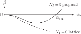
The precise determination of the mass and width of the $f_{0}(500)$ resonance [1, 2, 3] prompts us to revisit an old idea [5, 4] that the chiral condensate $\langle\bar{q}q\rangle_{\mathrm{vac}}\not=0$ may also be a condensate for scale transformations in the chiral $SU(3)_{L}\times SU(3)_{R}$ limit. This can occur in QCD if the heavy quarks $t,b,c$ are first decoupled and then the strong coupling¹¹ 1 We have $[D_{\mu}\,,\,D_{\nu}]=igG^{a}_{\mu\nu}T^{a}$ where $D_{\mu}$ is the covariant derivative, $\{T^{a}\}$ generate the gauge group, $\alpha_{s}=g^{2}/4\pi$ is the strong coupling, and $\beta=\mu\partial\alpha_{s}/\partial\mu$ and $\delta=-\mu\partial\ln m_{q}/\partial\mu$ refer to a mass-independent renormalization scheme with scale $\mu$. $\alpha_{s}$ of the resulting 3-flavor theory runs nonperturbatively to a fixed point $\alpha_{\mathrm{IR}}$ in the infrared limit (Fig. 1). At that point, $\beta(\alpha_{\mathrm{IR}})$ vanishes, so the gluonic term in the strong trace anomaly [9]

is absent, which implies

and hence a $0^{++}$ QCD dilaton²² 2 We reserve the term dilaton and notation $\sigma$ for a Nambu-Goldstone boson due to exact scale invariance in some limit. We are not talking about the $\sigma$-model, scalar gluonium [10], or “walking gauge theories” [11] where $\beta$ is small but never zero. $\sigma$ due to quark condensation.³³ 3 In field and string theory, it is often stated that Green’s functions are manifestly conformal invariant for $\beta=0$. That depends on the unlikely assumption that no scale condensates are present; otherwise, conformal invariance becomes manifest only if all 4-momenta are space-like and large. The obvious candidate for this state is the $f_{0}(500)$, which arises from a pole on the second sheet at a complex mass with typical value [1]

and surprisingly small errors [12]. In all estimates of this type, the real part of $m_{f_{0}}$ is less than $m_{K}$.

We begin by setting up chiral-scale perturbation theory $\chi$PT_σ for amplitudes expanded in $\alpha_{s}$ about $\alpha_{\mathrm{IR}}$. Its Lagrangian summarises soft-$\{\pi,K,\eta,\sigma\}$ meson theorems for approximate chiral $SU(3)_{L}\times SU(3)_{R}$ and scale symmetry, with results for strong interactions similar to those found originally [5, 4]. Effective weak operators are then added to simulate nonleptonic $K$ decays. The main result is a simple explanation of the $\Delta I=1/2$ rule for kaon decays: in leading order of $\chi$PT_σ, there is a dilaton pole diagram (Fig. 2) which accounts for the dominant $I=0$ amplitude.

It is well known that dispersive analyses which include $f_{0}(500)$ pole amplitudes produce excellent fits to data for $K\to\pi\pi$ [13, 14, 15] and $\gamma\gamma\to\pi\pi$ [16, 17] as well as $\pi\pi\to\pi\pi$. The problem is that, in the context of conventional chiral $SU(3)_{L}\times SU(3)_{R}$ perturbation theory $\chi$PT₃, these corrections are far too large.⁴⁴ 4 Similarly $\chi$PT₃ fails for $K_{L}\to\pi^{0}\gamma\gamma$ [18]. They cannot contribute to leading terms ${\cal A}_{\mathrm{LO}}$ in $\chi$PT₃ expansions

because $f_{0}$ does not belong to the $\chi$PT₃ Goldstone sector $\{\pi,K,\eta\}$. How can this be reconciled with the success [19] of $\chi$PT₃ elsewhere⁵⁵ 5 Except non-leptonic hyperon decays: either $\chi$PT for baryons or the weak sector of the Standard Model will have to be amended. where next to leading order terms ${\cal A}_{\mathrm{NLO}}$ are corrections $\lesssim$ 30%? The discrepancy is extreme for $K\to\pi\pi$: an $f_{0}$ pole in ${\cal A}_{\mathrm{NLO}}$ producing the factor of 22 enhancement of the $I=0$ amplitude would be $\approx$ 70 times the expected 30% correction.

Our solution to this problem is to replace $\chi$PT₃ with $\chi$PT_σ. We include $f_{0}=\sigma$ in the Goldstone sector $\{\pi,K,\eta,\sigma\}$ and identify scale invariance (Eq. (2)) as the symmetry most likely to permit this. The idea works because $\chi$PT_σ includes $f_{0}$ pole amplitudes in its leading order terms without upsetting successful leading order $\chi$PT₃ predictions for amplitudes which do not involve the $0^{++}$ channel; that is because the $\chi$PT₃ Lagrangian equals the $\sigma\to 0$ limit of the $\chi$PT_σ Lagrangian. In next to leading order, new chiral loop diagrams involving $\sigma$ need to be checked.

Notice that $\sigma$ becomes a Goldstone boson only if all three quarks $u,d,s$ become massless for $\alpha_{s}\to\alpha_{\mathrm{IR}}$.

In the limit $m_{u,d}\to 0$ with $m_{s}\not=0$, we use standard chiral $SU(2)_{L}\times SU(2)_{R}$ perturbation theory $\chi$PT₂, where momenta $i\partial$ are $O(m_{\pi})$ and the Goldstone sector is $\{\pi^{+},\pi^{0},\pi^{-}\}$. We do not include a dilaton in $\chi$PT₂: $f_{0}$ belongs to the non-Goldstone sector, so it retains most of its mass and width in that limit. $\chi$PT₂ is not sensitive to the behavior of $\beta$ because of the relatively large term $m_{s}\bar{s}s$ in Eq. (1) for $\theta^{\mu}_{\mu}$.

Consider strong interactions at low energies $\alpha_{s}\lesssim\alpha_{\mathrm{IR}}$ within the physical region

The gluonic trace anomaly is represented by a term $\mathcal{L}_{\mathrm{anom}}$ in an effective chiral-scale Lagrangian

constructed from a chiral invariant QCD dilaton field $\sigma$ and the usual chiral $SU(3)$ field $U=U(\pi,K,\eta)$. Both $\mathcal{L}_{\mathrm{inv}}$ and $\mathcal{L}_{\mathrm{anom}}$ are $SU(3)_{L}\times SU(3)_{R}$ invariant, while $\mathcal{L}_{\mathrm{mass}}$ belongs to the representation $(\mathbf{3},\bar{\mathbf{3}})\oplus(\bar{\mathbf{3}},\mathbf{3})$ associated with the $\pi,K,\eta$ (mass)² matrix $M$. The operator dimensions of $\mathcal{L}_{\mathrm{inv}}$ and $\mathcal{L}_{\mathrm{mass}}$ satisfy $d_{\mathrm{inv}}=4$ and $1\leqslant d_{\mathrm{mass}}<4$, with

as a result of expanding in $\alpha_{s}$ about $\alpha_{\mathrm{IR}}$. The dimension of $\mathcal{L}_{\mathrm{anom}}$ is found by noting that the gluonic anomaly corresponds to the $\beta\partial/\partial\alpha_{s}$ term in the Callan-Symanzik equation

for renormalization-group invariant QCD amplitudes $\mathcal{A}$. Taking $\partial/\partial\alpha_{s}$, we find

so for $\alpha_{s}\lesssim\alpha_{\mathrm{IR}}$, ${\cal L}_{\mathrm{anom}}$ has a positive anomalous dimension equal to the slope of $\beta$ at the fixed point (Fig. 1):

As $\alpha_{s}\to\alpha_{\mathrm{IR}}$, the gluonic anomaly vanishes, so for consistency, we must suppose that terms in ${\cal L}_{\mathrm{anom}}$ contain derivatives $O(\partial\partial)=O(M)$ or have $O(M)$ coefficients. The result is a chiral-scale perturbation expansion $\chi$PT_σ about $\alpha_{\mathrm{IR}}$ with QCD dilaton mass $m_{\sigma}=O(m_{K})$.

Note that QCD in the limit (2) resembles the physical theory in the resonance region, but differs completely at high energies because it lacks asymptotic freedom: instead, Green’s functions scale with nonperturbative anomalous dimensions. All particles except $\pi,K,\eta$ and $\sigma$ remain massive. Strong gluon fields set the scale of the condensate $\langle\bar{q}q\rangle_{\mathrm{vac}}$, which then sets the scale for massive particles and resonances except (possibly) glueballs.

An explicit formula for the $\chi$PT_σ Lagrangian (6) can be found by applying the method of Ellis [4, 20]. Let $F_{\sigma}$ be the coupling of $\sigma$ to the vacuum via the energy momentum tensor $\theta_{\mu\nu}$, improved [21] when spin-0 fields are present:

The dilaton field is given a scaling property $\sigma\to\sigma$ + {constant} such that $e^{\sigma/F_{\sigma}}$ has dimension $1$. Then the dimensions of chiral Lagrangian operators such as

and the dilaton operator $\mathcal{K}_{\sigma}=\frac{1}{2}\partial_{\mu}\sigma\partial^{\mu}\sigma$ can be adjusted by powers of $e^{\sigma/F_{\sigma}}$ to form terms in $\mathcal{L}$. In leading order,

where $\beta^{\prime}$ and $\delta$ are the anomalous dimensions $\beta^{\prime}(\alpha_{\mathrm{IR}})$ and $\delta(\alpha_{\mathrm{IR}})$ of Eqs. (10) and (7). The constants $c_{1}$ and $c_{2}$ are not fixed by general arguments, while $c_{3}$ and $c_{4}$ depend on how the field $\sigma$ is chosen. For the vacuum to be stable in the $\sigma$ direction at $\sigma=0$, terms linear in $\sigma$ must cancel:

Because of our requirement ${\cal L}_{\mathrm{anom}}=O(\partial^{2},M)$, both $c_{3}$ and $c_{4}$ are $O(M)$.

The critical exponent $\beta^{\prime}$ normalises the gluonic term in the trace of the effective energy-momentum tensor:

In leading order, $\cal L$ gives formulas for the $\sigma\pi\pi$ coupling

and dilaton mass $m_{\sigma}$

which resemble pre-QCD results [4, 5, 20, 22] but have extra gluonic terms proportional to $\beta^{\prime}$. We assume that the unknown coefficient $2+(1-c_{1})\beta^{\prime}$ in Eq. (16) does not vanish accidentally. That preserves the key feature of the original work, that $\mathcal{L}_{\sigma\pi\pi}$ is mostly derivative: for soft $\pi\pi$ scattering (energies $\sim m_{\pi}$), the dilaton pole amplitude is negligible because the $\sigma\pi\pi$ vertex is $O(m_{\pi}^{2})$, while the $\sigma\pi\pi$ vertex for an on-shell dilaton

is $O(m_{\sigma}^{2})$, consistent with $\sigma$ being the broad resonance $f_{0}(500)$.

Comparisons with data require an estimate of $F_{\sigma}$, most simply from $NN$ scattering and the dilaton relation

The data imply [23] a mean value $g_{\sigma NN}\sim 9$ and hence $F_{\sigma}\sim-100\,\mathrm{MeV}$ but with an uncertainty which is either model dependent or very large ($\approx 70\%$). That accounts for the large uncertainty in

when we compare Eq. (18) with $|g_{\sigma\pi\pi}|=3.31^{+0.35}_{-0.15}\,\mathrm{GeV}$ [2] and $m_{\sigma}\approx 441\,\mathrm{MeV}$.

The convergence of our chiral-scale expansion can be tested by adding $\sigma$-loop diagrams to the standard analysis [19, 24] for $\chi$PT₃. These involve the (as yet) undetermined constants $\beta^{\prime},\delta,c_{1\ldots 4}$: for example, corrections to $g_{\sigma\pi\pi}$ involve the $\sigma\sigma\sigma$ and $\sigma\sigma\pi\pi$ vertices derived from Eq. (13). However, when we apply the dimensional arguments of Manohar and Georgi [24] to our scheme, we find that there are two $\chi$PT_σ scales $\chi_{\pi}=4\pi F_{\pi}$ and $\chi_{\sigma}=4\pi F_{\sigma}$, which are numerically similar ($F_{\sigma}\sim F_{\pi}$). The following points should be noted:

1. 1.

   The $\alpha_{s}\lessapprox\alpha_{IR}$ scales $\chi_{\pi,\sigma}\approx$ 1 GeV must not be confused with the scale $\Lambda_{\mathrm{QCD}}\approx$ 200 MeV for ultraviolet expansions $\alpha_{s}\gtrapprox 0$ (asymptotic freedom).

2. 2.

   The small value of $F_{\sigma}\ll\chi_{\pi,\sigma}$ implies a $\sigma$ width

   $$\Gamma_{\sigma\pi\pi}\approx\frac{|g_{\sigma\pi\pi}|^{2}}{16\pi m_{\sigma}}\sim\frac{m_{\sigma}^{3}}{16\pi F_{\sigma}^{2}}\sim 250\mbox{ MeV}$$

   (21)

   which is numerically misleading: $\Gamma_{\sigma\pi\pi}$ is $O(m_{\sigma}^{3})$ and hence non-leading relative to the mass $m_{\sigma}$. So tree diagrams produce the leading order⁶⁶ 6 Beyond leading order, and in degenerate cases like the $K_{L}$–$K_{S}$ mass difference, methods used to estimate corrections at the $Z^{0}$ peak [25] and the $\rho$ resonance [26] may be necessary. of $\chi$PT_σ, as in $\chi$PT₂ and $\chi$PT₃.

3. 3.

   The technique used to obtain Eq. (13) from $\chi$PT₃ also works for $O(\partial^{4},M\partial^{2},M^{2})$ terms in $\cal L$ (and in ${\cal L}_{\mathrm{weak}}$ below). For example, a term $\sim(\mbox{Tr}\partial U\partial U^{\dagger})^{2}$ appears in ${\cal L}^{d=4}_{\mathrm{inv,NLO}}$ without $\sigma$-field dependence, but within ${\cal L}^{d>4}_{\mathrm{anom,NLO}}$, it becomes⁷⁷ 7 To the extent allowed by data for soft-$\sigma$ amplitudes, $O(\partial^{4})$ coefficients can be predicted by saturation by non-Goldstone resonances — like $\chi$PT₃ [27], but with $f_{0}$ excluded.

   $$\{\mbox{coefficient}\}\bigl(\mbox{Tr}\partial U\partial U^{\dagger}\bigr)^{2}e^{\beta^{\prime}\sigma/F_{\sigma}}.$$

   (22)

The most important feature of $\chi\mathrm{PT}_{\sigma}$ is that it explains the $\Delta I=1/2$ rule for $K\rightarrow\pi\pi$ decays.

In the leading order of standard $\chi$PT₃, the effective weak Lagrangian

contains an octet operator [28]

the $U$-spin triplet component [29, 30] of a 27 operator

and a weak mass operator [31]

Although $Q_{M}$ has isospin 1/2, it cannot be used to solve the $\Delta I=1/2$ puzzle if dilatons are absent: when $Q_{M}$ is added to the strong mass term $\left.{\cal L}_{\mathrm{mass}}\right|_{\sigma=0}$, it can be removed by a chiral rotation which aligns the vacuum [30] such that $\langle U\rangle_{\mathrm{vac}}=I$ and $M$ = real diagonal. Therefore the conclusion that $|g_{8}/g_{27}|$ is unreasonably large ($\approx$ 22) is not avoided.

In $\chi$PT_σ, the outcome is entirely different. The weak mass operator’s dimension $(3+\delta_{w})$ is not the same as the dimension $(3+\delta)$ of ${\cal L}_{\mathrm{mass}}$, so the $\sigma$ dependence of $Q_{M}e^{(3+\delta_{w})/F_{\sigma}}$ cannot be eliminated by a chiral rotation. Instead, after aligning the vacuum, we find

noting that $Q_{8}$ represents quark-gluon operators with differing dimensions at $\alpha_{\mathrm{IR}}$. As a result, there is a residual interaction $\mathcal{L}_{K_{S}\sigma}=g_{K_{S}\sigma}K_{S}^{0}\sigma$ which mixes $K_{S}$ and $\sigma$ in leading order

and produces the $\Delta I=1/2$ amplitude $A_{\sigma\textrm{-pole}}$ of Fig. 2.

From $\gamma\gamma\rightarrow\pi^{0}\pi^{0}$ and $K_{S}^{0}\rightarrow\gamma\gamma$ (Fig. 3), we estimate

to about 30% precision and so, to the extent that $g_{\sigma NN}$ and hence $F_{\sigma}$ can be determined,

This accounts for the large $I=0\ \pi\pi$ amplitude $A_{0}$ [3]

compared with $A_{2}$. So we conclude that the observed ratio $|A_{0}/A_{2}|\simeq 22$ is mostly due to the dilaton-pole diagram of Fig. 2, that $g_{8}=\sum_{n}g_{8n}$ and $g_{27}$ may have similar magnitudes as simple calculations indicate, and that only $g_{27}$ can be fixed precisely (from $K^{+}\rightarrow\pi^{+}\pi^{0}$).

Consequently, the leading order of $\chi$PT_σ solves the $\Delta I=1/2$ problem for kaon decays. The chiral Ward identities which relate the on-shell $K\to 2\pi$ and $K\to\pi$ amplitudes have extra terms due to $\sigma$ poles, but the no-tadpoles theorem [30] is still valid:

The presence of the $\sigma\gamma\gamma$ vertex in Fig. 3 leads us to apply the electromagnetic trace anomaly [33, 34]

to QCD at the infrared fixed point $\alpha_{s}=\alpha_{\mathrm{IR}}$. Here $F_{\mu\nu}$ and $\alpha$ are the electromagnetic field strength tensor and fine-structure constant.

The $\chi$PT_σ result for the $\sigma\gamma\gamma$ amplitude is affected by the observation [32] that in $\gamma\gamma$ channels, charged $\pi,K$ loop diagrams are finite in the chiral limit. This means that they are of the same order as $\sigma$-pole diagrams: partial conservation of the dilatation current is not equivalent to simple $\sigma$-pole dominance in $\gamma\gamma$ channels. The electromagnetic trace anomaly remains the same (with $R\to R_{\mathrm{IR}}$), but because of the extra $(\pi^{\pm},K^{\pm})$ loops in $\langle\gamma\gamma|\theta^{\mu}_{\mu}|\mathrm{vac}\rangle$, the $\sigma\gamma\gamma$ coupling is proportional to $R_{\mathrm{IR}}-\frac{1}{2}$, not $R_{\mathrm{IR}}$:

Evidently, data used to estimate $|g_{K_{S}\sigma}|$ can also be used to find a phenomenological value for $R_{\mathrm{IR}}$. In a dispersive analysis of $\gamma\gamma\to\pi\pi$, it was shown [16] that the residue of the $f_{0}(500)$ pole can be extracted from the Crystal Ball data [35]. We use an updated value [17] of the width $\Gamma(f_{0}\rightarrow\gamma\gamma)=1.98^{+0.30}_{-0.24}$ keV. Within the large uncertainty due to that in $F_{\sigma}$, we find:

This result is a feature of the non-perturbative theory at $\alpha_{\mathrm{IR}}$, so it has nothing to do with asymptotic freedom or the free-field formula $(N_{f}=3)$

Notice that $\chi$PT_σ relates amplitudes in the physical region (5) to high-energy quantities like $\delta(\alpha_{\mathrm{IR}})$ and $R_{\mathrm{IR}}$ characteristic of massless QCD at $\alpha_{\mathrm{IR}}$. Does QCD simplify in that limit and, unlike QED [36], allow $\beta^{\prime}\not=0$ at the fixed point?

Unfortunately, our analysis does not explain the failure of chiral theory to account for non-leptonic $|\Delta S|=1$ hyperon decays. We have shown that octet dominance is not necessary, but that makes no difference for hyperon decays: the Pati-Woo $\Delta I=1/2$ mechanism [37] forbids all contributions from 27 operators.