Accessible nonlinear entanglement witnesses

Entangled states are an important resource for performing quantum information processing tasks [1]. As a tool for characterization of this resource entanglement verification finds broad application in theoretical and practical testing of quantum resources and devices, such as quantum memories, quantum repeaters or quantum channels [2, 3], which are essential for the creation, storage and distribution of quantum information.

In experimentally relevant scenarios entanglement witnesses (EW) are playing a central role as a tool for entanglement detection [1, 4]. Recently, a theoretical construction has been suggested which extends witnesses that use linear combinations of observed expectation values to those using nonlinear functions [5, 6, 7]. The nonlinear extension of a linear EW is stronger in the sense that it detects a strictly larger set of entangled states. However, the evaluation of a generic nonlinear extension will typically require additional measurements compared to the evaluation of the linear EW. This fact can be a drawback for experimental applications.

In all experiments for entanglement detection which use EWs as a tool, the observable corresponding to the witness is not measured directly. Instead, the EW observable is decomposed in terms of local observables. Then, one performs a series of measurements corresponding to the measurement of each term in the decomposition. Such a decomposition is not unique and can be chosen according to the specific nature of the experiment [1].

The problem of entanglement detection with a fixed restricted set of measurements has been already addressed in Ref. [8]. Investigation of this problem naturally leads to the definition of verifiable states. For the given set of restricted measurements a state is called verifiable if the outcomes of the measurements are not compatible with the outcomes of the same measurements on any separable state. The set of all linear witnesses which can be constructed from this restricted set of measurements is called the verification set. Characterizing the verification set or finding a witness for a given verifiable state is a challenging problem [8], which is in fact as hard as finding an EW for an arbitrary entangled state [4].

Here we introduce a framework for the entanglement detection when only a restricted set of local observables is measured and no further knowledge about the state can be obtained. It leads to a family of easily computable entanglement criteria - accessible nonlinear EWs. Accessibility of a nonlinear witness (for which a rigorous definition is given later) refers to the fact that it can be written as a rational function of expectation values that can be accessed by just performing the restricted set of measurements, i.e. the same measurements that are necessary for the evaluation of the linear EW. As the range of detected states is significantly extended for non-linear witnesses, we can to some degree avoid the problem of searching through the verification set of linear witnesses. This comes at the price that not all verifiable states will be detected. Furthermore we address the question under which conditions an accessible nonlinear EW can be constructed. In a general scenario we provide sufficient conditions for the accessibility of the nonlinear extension. For several relevant but more specific scenarios we find necessary conditions as well. Besides, accessible nonlinear EWs turn out to have higher detection significance when evaluated from the experimental data.

Main idea.- Let us first introduce some notation. Denote by $\mathcal{H}_{A}$ ($\mathcal{H}_{B}$) Hilbert space of dimension $d_{A}$ ($d_{B}$) and by $\mathcal{B}(\mathcal{H}_{A})$ ($\mathcal{B}(\mathcal{H}_{B})$) the set of all bounded linear operators on the corresponding Hilbert space. Quantum states on a bipartite Hilbert space $\mathcal{H}_{AB}$ are described by positive semi-definite operators with unit trace and denoted by $\rho_{AB}$. A linear EW on $\mathcal{H}_{AB}$ is a Hermitian operator $W_{AB}$, such that

Initial work on non-linear witnesses [5] concentrated on extension of linear witnesses that were equivalent to some negative partial transposition criterion. Subsequently, it was pointed out that by employing Choi-Jamiołkowski isomorphism [9, 10] it is in principle possible to construct nonlinear improvements for any given linear EW [11]. We will review nonlinear witnesses using this generalized view. Any entanglement witness $W_{AB}\in\mathcal{B}(\mathcal{H}_{A}\otimes\mathcal{H}_{B})$ is equivalent to a positive but not completely positive (PnCP) map $\Lambda_{W}:\mathcal{B}(\mathcal{H}_{A})\rightarrow\mathcal{B}(\mathcal{H}_{B})$ via the following relationship

for any $X_{A}\in\mathcal{B}(\mathcal{H}_{A})$, where the partial transposition is taken w.r.t. an orthonormal basis $\{|k\rangle_{k=1}^{d_{A}}\}$. Due to the isomorphism of the map $W_{AB}\mapsto\Lambda_{W}(.)$ the witness is restored by applying an extension of $\Lambda_{W}$ to the projector onto the maximally entangled state on $\mathcal{H}_{AA^{\prime}}$, where $\mathcal{H}_{A^{\prime}}\cong\mathcal{H}_{A}$,

In the remainder of the paper we will omit the subscript $AB$ of $W$, unless we state explicitly to which two parties we refer to, while keeping in mind that $W$ always acts on a bipartite Hilbert space $\mathcal{H}_{AB}$ and the extension of the map $\tilde{\Lambda}$, corresponding to $W$, acts always from $\mathcal{H}_{AA^{\prime}}$ to $\mathcal{H}_{AB}$.

In order to derive a nonlinear EW we first note that $\mbox{Tr}\left(\rho\mathcal{O}\mathcal{O}^{\dagger}\right)$ is positive semi-definite for any state $\rho$ and any operator $\mathcal{O}$. As a consequence, for any decomposition $\mathcal{O}=\sum_{i=1}^{n}c_{i}\mathcal{O}_{i}$ with free parameters $c_{i}$ and any set of operators $\mathcal{O}_{i}$, this is equivalent to the positive semi-definiteness of a matrix $M_{\rho}=\left\{\mbox{Tr}\left(\rho\mathcal{O}_{i}\mathcal{O}^{\dagger}_{j}\right)\right\}_{i,j=1}^{n}$. Then, by choosing $\mathcal{O}_{1}$ as the projector onto the maximally entangled state $\mbox{P}_{\Psi^{+}}$ and $\mathcal{O}_{2}$ as some unitary $U$ we see that for all separable bipartite states $\rho_{s}\in\mathcal{B}(\mathcal{H}_{AB})$ the matrix

must be positive semi-definite [7]. Here we introduced $\tilde{\Lambda}^{\dagger}$ as the adjoint map of $\tilde{\Lambda}$. Since, $\Lambda_{W}$ is a PnCP map $\tilde{\Lambda}_{W}$ will transform separable states into positive operators, and so will its adjoint $\tilde{\Lambda}^{\dagger}$. Therefore for general bi-partite states $\rho$, failure of the matrix in Eq. (Accessible nonlinear entanglement witnesses) to be positive is a conclusive proof that that particular $\rho$ must be entangled. By using the definition of the adjoint map again, while noting that $\tilde{\Lambda}_{W}[\mbox{P}_{\Psi_{AA^{\prime}}^{+}}]=W_{AB}$ and assuming that $\mbox{Tr}\left(\rho\tilde{\Lambda}_{W}[\mathbbm{1}]\right)\neq 0$, we construct from the determinant of Eq. (Accessible nonlinear entanglement witnesses) a nonlinear function which improves the entanglement detection given by the linear EW,

That is, if for some $U$ we have that $w_{NL}(\rho)<0$, then the state $\rho\in\mathcal{B}(\mathcal{H}_{AB})$ must be entangled. The new criterion (6) detects more entangled states, for we subtract a strictly positive number from the expectation value of $W$.

The quantity $w_{NL}(\rho)$ can be represented as an expectation value of an operator $W_{NL}$, which we call a nonlinear EW. From Eq. (6) it is straightforward to verify that $W_{NL}$ is given by

The case of $\varkappa\neq 1$ reveals the fact that $\Lambda_{W}$ can be non-unital, meaning that $\tilde{\Lambda}_{W}$ does not necessarily map the identity onto the identity.

Let us mention some facts about the nonlinear EWs. To begin with, note that Eq. (6) can be easily iterated in a similar way as it is done in Ref. [7]. There, for example, nonlinear improvements for all fully PPT witnesses [12, 13], i.e. EWs of the form $W=P^{\Gamma}$, with $P\geq 0$ and $\Gamma$ the partial transposition w.r.t. either of parties, were considered. The iteration process in the general case is established by defining

Then the $n$th nonlinear improvement is given by $W_{n}:=\tilde{\Lambda}_{W}[Q_{n}Q_{n}^{\dagger}]$. Moreover, a simple calculation shows that $w_{n}(\rho):=\mbox{Tr}\left(\rho W_{NL}\right)$ is given by a recurrence relation

with

If $w_{n}(\rho)<0$ for some $n$ then $\rho$ must have been entangled.

The evaluation of the quantities $w_{n}(\rho)$ in general would require the knowledge of the whole density matrix. In order to overcome this restrictive circumstance, we can employ the aforementioned fact that the linear witnesses are not measured directly but rather decomposed in a linear combination of local measurable observables which are then measured. Therefore the starting point of all our studies will be always a particular decomposition of a linear EW in terms of the local observables $A_{i}\in\mathcal{B}(\mathcal{H}_{A})$ and $B_{i}\in\mathcal{B}(\mathcal{H}_{B})$ on Alice’s and Bob’s side. Let us write this decomposition as $W=\sum_{i=1}^{N}c_{i}A_{i}\otimes B_{i}$. By measuring the observables $\{A_{i}\otimes B_{i}\}_{i=1}^{N}$ we naturally induce a linear and, in general, not injective map $\mathcal{M}:\rho\mapsto\mathcal{M}(\rho)\in\mathbbm{R}^{N}$, where the space $\mathbbm{R}^{N}$ consists of the expectation values of observables $\{A_{i}\otimes B_{i}\}_{i=1}^{N}$ in all possible physical states $\rho\in\mathcal{B}(\mathcal{H}_{AB})$ [8]. The map $\mathcal{M}$ maps a convex set of separable states $S$ onto a convex set $S^{\prime}=\mathcal{M}(S)\in\mathbbm{R}^{N}$ - the equivalence class of all separable states that are compatible with the expectation values $\{\langle A_{i}\otimes B_{i}\rangle\}_{i=1}^{N}$. The set of all linear EWs $W=\sum_{i=1}^{N}\alpha^{W}_{i}A_{i}\otimes B_{i}$ for different coefficients $\{\alpha_{i}^{W}\}$ form the verification set and are equivalent to a set of hyper-planes in $\mathbbm{R}^{N}$, each dividing $\mathbbm{R}^{N}$ into two halves, one of which contains the set $S^{\prime}$ [8].

It is evident now that no additional measurements are needed if $w_{n}(\rho)$ can be evaluated from the expectation values $\{\langle A_{i}\otimes B_{i}\rangle\}_{i=1}^{N}$ only and, therefore, defines a hyper-surface in $\mathbbm{R}^{N}$. This leads us to the definition of an accessible nonlinear EW as a nonlinear improvement of a linear EW from the verification set.

As we will show now, it is possible to formulate conditions when the knowledge of the set of expectation values $\{\langle A_{i}\otimes B_{i}\rangle\}_{i=1}^{N}$ is sufficient (and in some cases even necessary and sufficient) for the calculation of $w_{n}(\rho)=\mbox{Tr}\left(W_{n}\rho\right)$.

Our first goal is to find the conditions when, for the first step of the iteration, $w_{NL}(\rho)$ in Eq. (6) can be written as a rational function in the space $\mathbbm{R}^{N}$ that is defined by the restricted set of measurements. For that it is sufficient to show that the operators $\tilde{\Lambda}_{W}[\mbox{P}_{\Psi^{+}}U]$ and $\tilde{\Lambda}_{W}[\mathbbm{1}]$ can be decomposed only in terms of the observables $\{A_{i}\otimes B_{i}\}_{i=1}^{N}$. This will imply that the quadratic term in Eq. (6) can be computed from the expectation values $\langle A_{i}\otimes B_{i}\rangle_{\rho}$ and no further measurements are needed or equivalently that $w_{NL}(\rho)$ is a rational function in $\mathbbm{R}^{N}$.

Formally, the sufficient condition from the previous paragraph can be grasped by the following Observation.

Proof: First note that $\mbox{P}_{\Psi^{+}}\in V^{\prime}$, since $\tilde{\Lambda}_{W}[\mbox{P}_{\Psi^{+}}]=W\in V$. As $V^{\prime}$ is an unital algebra and $U\in V^{\prime}$ it follows that $\mathbbm{1},\mbox{P}_{\Psi^{+}}U\in V^{\prime}$ and therefore $\tilde{\Lambda}_{W}[\mathbbm{1}]$, $\tilde{\Lambda}_{W}[\mbox{P}_{\Psi^{+}}U]\in V$. This implies that the operator $\tilde{\Lambda}_{W}[\mbox{P}_{\Psi^{+}}U]$ can be decomposed in terms of local observables $\{A_{i}\otimes B_{i}\}_{i=1}^{N}$ only and $w_{NL}(\rho)$ is accessible. $\hfill\blacksquare$

Furthermore, if the conditions of Observation 2 are fulfilled, then $w_{n}(\rho)$ represents an accessible nonlinear EW for any $n$. This can be readily shown by applying the method of the mathematical induction in $n$. Since the conditions of Observation 2 hold, the definition of the operator $Q_{1}$ implies that it lies in the algebra $V^{\prime}$ and therefore $w_{1}(\rho)$ is accessible. Thus if $Q_{n-1}$ lies in $V^{\prime}$ and $U_{n-1}\in V^{\prime}$ so does $Q_{n}$, which implies that $w_{n}(\rho)$ is accessible. Formally we have:

Before we go over to examples of accessible nonlinear witnesses, we will now provide structures that are useful for these examples and many experimental implementations.

An analytical formula for the iterations.- For a special choice of unitary operators in the iteration process, $\lim_{n\rightarrow\infty}w_{n}$ can be calculated analytically and gives a strong accessible nonlinear EW.

Proof: In order to prove the statement first note that by applying twice the recurrence relation Eq. (8) to $\mbox{Tr}\left(\rho\tilde{\Lambda}_{W}[Q_{n}]\right)$, while keeping in mind that $U_{n}^{2}=\mathbbm{1}$, we have $\mbox{Tr}\left(\rho\tilde{\Lambda}_{W}[Q_{n}]\right)=0$ for all $n>1$. Hence, by using the same recurrence relation again we immediately see that the coefficients $c_{n}(\rho)$ form a geometric progression $c_{n}(\rho)=\varkappa^{2}|k(\rho)|^{2}c_{n-1}(\rho)$. Thus $w_{n}(\rho)=\mbox{Tr}\left(W\rho\right)-\varkappa|c(\rho)|^{2}-\varkappa|d(\rho)|^{2}\sum_{m=1}^{n-1}(\varkappa|k|)^{2(m-1)}$. Taking the limit $n\rightarrow\infty$ proves the claim.$\hfill\blacksquare$

Notably, for the special choice of the unitary as in Proposition 4, we can strengthen Observation 2 and formulate conditions which are necessary and sufficient for the evaluation of the analytical formula.

Proof: First assume that $k(\rho)$, $\varkappa(\rho)$ and $d(\rho)$ are accessible. Then $w_{n}(\rho)$ must be accessible as it is a function of $k(\rho),\varkappa(\rho)$ and $d(\rho)$ only, for all values of $n$. This finishes the first part of the proof.

Now assume every $w_{n}(\rho)$ is accessible. Define $v_{i}:=\mbox{Tr}\left(\rho A_{i}\otimes B_{i}\right)$ and $z_{j}:=\mbox{Tr}\left(\rho Z_{j}\right)$ where the set of hermitian operators $\{Z_{j}\}$ form a basis of the orthogonal complement $V^{\perp}$ of $V=\mbox{span}\{A_{i}\otimes B_{i}\}_{i=1}^{N}$. Then a quantity $q(\{v_{i}\},\{z_{i}\})$ is accessible if it can be expressed as a function of the variables $v_{i}$ only. Equivalently one can say that all derivatives of $q$ with respect to every $z_{j}$ must vanish for all values of the variables $\{v_{i}\}$ and $\{z_{j}\}$.

First note that for $c(\rho)=0$, we find that $w_{n}(\rho)=w_{0}(\rho)$ for all $n$ and for any values of $\varkappa(\rho)$ and $k(\rho)$, since $c_{n}(\rho)=\varkappa^{2}|k|^{2}c_{n-1}(\rho)$ when $U_{n}^{2}=\mathbbm{1}$. In this case the nonlinear improvements coincide with the expectation value of the linear witness and therefore do not provide any advantage, so we do not have to worry about the accessibility of $\varkappa(\rho)$ and $k(\rho)$ at all. So from now on we can assume that $c(\rho)\neq 0$ whenever necessary.

In general, we can write $c=\sum_{i}a_{i}v_{i}+\sum_{j}x_{j}z_{j}$ and $\varkappa^{-1}=\sum_{i}b_{i}v_{i}+\sum_{j}y_{j}z_{j}$ for some fixed numbers $\{a_{i}\},\{x_{j}\},\{b_{i}\},\{y_{j}\}$. We want to show that $x_{j}=y_{j}=0$ for all values of $j$. Using the fact that $w_{1}$ and $\mbox{Tr}\left(\rho W\right)$ are accessible together with the above expressions for $c$ and $\varkappa^{-1}$ one can show that the condition $\frac{\partial}{\partial z_{l}}\varkappa|c|^{2}=0$, for any $l=1,\ldots,dim(V^{\perp})$ is equivalent to the system of linear equations

where

Recall from (6) that we always have $\varkappa^{-1}=\gamma_{l}+y_{l}z_{l}\neq 0$ and therefore Eqns. (12) and (13) imply $|x_{l}|=0$ (otherwise both $\gamma_{l}$ and $y_{l}$ must be equal to zero, which would imply $\varkappa^{-1}=0$). Since this holds for any arbitrary $l$, it proves that $d$ is accessible. Further, because of $|x_{l}|=0$, Eq. (16) becomes $\beta_{l}=0$ and Eq. (15) becomes $\alpha_{l}=\sum_{i}\sum_{j}a_{i}a_{j}^{*}v_{i}v_{j}=|c|^{2}$. Moreover Eq. (14) gives $\alpha_{l}y_{l}=0$. Since $\alpha_{l}=|c|^{2}\neq 0$ it must be that $y_{l}=0$ for all values of $l$. This proves that $\varkappa$ is also accessible. Finally, using the fact that $w_{2}$ and $w_{3}$ are accessible, it is straightforward to show that $\varkappa|k|$ is accessible and this implies that $k$ is accessible as well. $\hfill\blacksquare$

Examples.- As a first example we consider an optimal decomposable witness for two qubits $W_{0}=P^{\Gamma}$, where $P$ is a positive semi-definite operator and $\Gamma$ denotes the partial transposition w.r.t. either one of the qubits [14]. Note that transposition is a PnCP map that leads to a necessary and sufficient criterion for entanglement detection in two qubit case [15]. The decomposition of such two-qubit EW in terms of local observables has been extensively studied. Let us consider an EW with the decomposition of the form $W_{0}=(\mathbbm{1}+\sum_{\alpha=x,y,z}\sigma_{\alpha}\otimes\sigma_{\alpha})/4$. This is an optimal entanglement witness [16, 17]. This EW does not detect the entanglement of the state $(|00\rangle+|11\rangle)/\sqrt{2}$, which is one of the Bell states. However, that entanglement is detected by the nonlinear improvement in Eq. (11). Indeed $\tilde{\Lambda}_{W}$ corresponds to the partial transposition and consequently $\varkappa^{-1}=1$. Direct calculation for the choice $U=(\mathbbm{1}+\sum_{\alpha=\{x,y,z\}}\sigma_{\alpha}\otimes\sigma_{\alpha})/2$ which satisfies $U^{2}=\mathbbm{1}$, gives $|k|=1$, with $d(\rho)\neq 0$ and hence $w_{\infty}(\rho)=-\infty$, meaning that the state is detected by the constructed accessible nonlinear EW $w_{\infty}(\rho)$.

In Fig. 1 we illustrate the results for a particular family of the states $\rho(\varphi)=(2/3)|\varphi\rangle\langle\varphi|+(1/12)\mathbbm{1}$, with $|\varphi\rangle=\frac{1}{\sqrt{2}}(|01\rangle-e^{i\varphi}|10\rangle)$ with $\varphi\in[0,2\pi]$. The value of the white noise admixture has been chosen to demonstrate a typical behavior. As we see, the linear witness detects entanglement only outside some interval containing $[\pi/2,3\pi/2]$, while the accessible nonlinear extension detects most entanglement within the interval. Note that the state is entangled for all values of $\varphi$, so this particular nonlinear extension does not detect all entanglement.

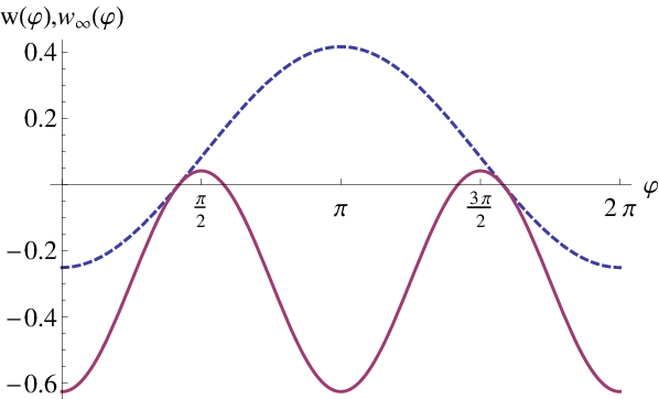
This example provides a nice demonstration of the general fact that the accessible nonlinear EWs always detect more states than their linear ancestors.

As our second example we consider improvements for a particular decomposition of a witness that detects bound entanglement in the four qubit Smolin state $\rho_{S}=\frac{1}{4}\sum_{k=0}^{3}|\Psi_{k}\rangle\langle\Psi_{k}|_{12}\otimes|\Psi_{k}\rangle\langle\Psi_{k}|_{34}$ [18]. Notably this state was recently prepared in the lab and its bound entanglement was confirmed experimentally [19]. The witness $W$ with the decomposition $W=\frac{1}{16}(\mathbbm{1}-\sum_{\alpha=x,y,z}\sigma_{\alpha}^{\otimes 4})$ is optimal for this state [20].

An accessible nonlinear witness can be derived from this witness decomposition by choosing the unitaries $U_{n}=(\mathbbm{1}+\sigma_{x}\otimes\sigma_{x}+\sigma_{y}\otimes\sigma_{y}+\sigma_{z}\otimes\sigma_{z})/2$ for all $n$ and constructed the nonlinear EW according to Eq. (11). In Fig. 2 we present a numerical calculation for the detection of the Smolin state mixed with the white noise $\rho_{S}(p)=(1-p)\rho_{S}+p\mathbbm{1}/16$ depending on the noise parameter $p$. The expectation value of the linear EW is represented by the line $w(p)$ and its improvement by the curve $w_{\infty}(p)$. Both witnesses tolerate a critical amount of noise of $p=2/3$ as the linear witness happens to be optimal at that point. Other types of noise would reveal the advantage of the nonlinear improvement in a manner similar to the example in Fig. 1.

Volume of detectable states and detection significance of the accessible nonlinear EWs.-

For the entanglement verification in experiments, detection significance is an important issue, which has to be addressed. The common and widely used approach to put error bars on the measured data - the Gaussian error propagation (see e.g. [21]), has recently lead to somewhat counterintuitive statements, stating, for example, that the smaller negative value of a linear entanglement witness does not necessarily imply higher detection significance [22].

In order to make reliable and meaningful statements for detection significance in entanglement verification experiments one ought to apply a more consistent framework. Such a framework has been recently presented by M. Christandl and R. Renner in Ref. [23]. There, the outcomes of $n$ runs of an experiment leads to an estimate density $\mu_{n}(\rho)$, which can be seen as a measure on the space of all states. According to Chapter 6 in Ref. [23] we assign the probability for a state to be in a subset $\Gamma$ of the state space w.r.t. the estimate density $\mu_{n}(\rho)$ as follows:

This picture can be related to the detection significance provided by the entanglement witnesses in the following sense. Denote by $\Gamma_{W}$ the set of all states that are detected by a witness $W$. According to Christandl-Renner framework any measured state will give rise to an estimate density $\mu_{n}$ which is typically non-zero on the whole state space. Then the detection significance of the state is given by $P_{\mu_{n}}(\Gamma_{W})$. Moreover, we say that a state is detected with a high significance if $P_{\mu_{n}}(\Gamma_{W})=1-\epsilon_{W}$, where $\epsilon_{W}$ is small comparing to 1.

From the previous considerations and from our first example it is clear that the volume of the states detected by the accessible nonlinear EW always includes the volume of the states detected by its linear ancestor. Interestingly, analyzed according to the framework of Ref. [23] the detection significance can only increase for accessible nonlinear EWs. Indeed, denote by $\Gamma_{W}$ and $\Gamma_{W_{NL}}$ the sets of states that are detected by the linear and the accessible nonlinear EW respectively. Then, since $\Gamma_{W}$ is strictly contained in $\Gamma_{W_{NL}}$, for any state we have

and the detection efficiency of the accessible nonlinear EW is strictly bigger than the detection efficiency of the linear EW.

Possible extensions and outlook.- The theory developed in this paper may be applied to a wide range of linear EWs and various examples of accessible nonlinear EWs can be constructed. One of the open questions which is worth investigating is whether for a given decomposition of a linear EW there exists an accessible non-linear extension. Moreover, it is interesting to understand if it is possible or not to construct nonlinear improvements which would detecting genuine multipartite entanglement.

Conclusion.- In this paper we investigated the separability of quantum states with only a restricted set of measurements using accessible nonlinear EWs. We have demonstrated that accessible nonlinear EWs detect entanglement in many states, which are not detected by the initial EW.

Moreover, we provided error analysis for the accessible nonlinear EWs and showed that the detection is performed with high statistical significance.

Therefore our framework provides a new systematic approach for studying entanglement of bipartite quantum systems both in theory and in experiment.

Acknowledgements.- We thank T.Moroder, O. Gühne and M. Piani for fruitful discussions. This work has been supported by the Industry Canada and NSERC Strategic Project Grant (SPG) FREQUENCY.

References

- [1] O. Gühne and G. Toth, Physics Reports 474, 1 (2009), ISSN 0370-1573.
- [2] N. Killoran, D. N. Biggerstaff, R. Kaltenbaek, K. J. Resch, and N. Lütkenhaus, Phys. Rev. A 81, 012334 (2010a).
- [3] N. Killoran, H. Häseler, and N. Lütkenhaus, Phys. Rev. A 82, 052331 (2010b).
- [4] R. Horodecki, P. Horodecki, M. Horodecki, and K. Horodecki, Rev. Mod. Phys. 81, 865 (2009).
- [5] O. Gühne and N. Lütkenhaus, Phys. Rev. Lett. 96, 170502 (2006).
- [6] O. Gühne and N. Lütkenhaus, Journal of Physics: Conference Series 67, 012004 (2007), ISSN 1742-6588.
- [7] T. Moroder, O. Gühne, and N. Lütkenhaus, Phys. Rev. A 78, 032326 (2008).
- [8] M. Curty, O. Gühne, M. Lewenstein, and N. Lütkenhaus, Phys. Rev. A 71, 022306 (2005).
- [9] A. Jamiołkowski, Rep. Math. Phys. 3, 275 (1972).
- [10] M. Lewenstein, B. Kraus, J. I. Cirac, and P. Horodecki, Phys. Rev. A 62, 052310 (2000).
- [11] O. Gühne, M. Mechler, G. Tóth, and P. Adam, Phys. Rev. A 74, 010301 (2006).
- [12] B. Jungnitsch, T. Moroder, and O. Gühne, Phys. Rev. Lett. 106, 190502 (2011a).
- [13] B. Jungnitsch, T. Moroder, and O. Gühne, arXiv:1106.1114 (2011b).
- [14] R. Augusiak, G. Sarbicki, and M. Lewenstein, arXiv:1107.0505 (2011).
- [15] A. Peres, Phys. Rev. Lett. 77, 1413 (1996).
- [16] O. Gühne, P. Hyllus, D. Bruß, A. Ekert, M. Lewenstein, C. Macchiavello, and A. Sanpera, Phys. Rev. A 66, 062305 (2002).
- [17] O. Gühne, P. Hyllus, D. Bruß, A. Ekert, M. Lewenstein, C. Macchiavello, and A. Sanpera, J. Mod. Opt. 50, 1079 (2003).
- [18] J. A. Smolin, Phys. Rev. A 63, 032306 (2001).
- [19] J. Lavoie, R. Kaltenbaek, M. Piani, and K. J. Resch, Phys. Rev. Lett. 105, 130501 (2010).
- [20] A. O. Pittenger and M. H. Rubin, Linear Algebra and its Applications 346, 47-71. (2002).
- [21] W. Eadie, D. Drijard, F. James, M. Roos, and B. Sadoulet, Statistical Methods in Experimental Physics (North-Holland Publishing Co., 1971).
- [22] B. Jungnitsch, S. Niekamp, M. Kleinmann, O. Gühne, H. Lu, W. Gao, Y. Chen, Z. Chen, and J. Pan, Phys. Rev. Lett. 104, 210401 (2010).
- [23] M. Christandl and R. Renner, arXiv:1108.5329 (2011).