跳到论文正文
W Papers独立论文阅读器 arXiv:1203.1180 论文正文 计算阅读时间 · 0%
引用这篇论文根据当前论文元数据生成,正式投稿前建议核对。


License: arXiv.org perpetual non-exclusive license
arXiv:1203.1180v1 [cs.RO] 06 Mar 2012

Incremental Temporal Logic Synthesis of Control Policies for Robots Interacting with Dynamic Agents

Tichakorn Wongpiromsarn    Alphan Ulusoy    Calin Belta    Emilio Frazzoli    Daniela Rus ††thanks: T. Wongpiromsarn is with the Singapore-MIT Alliance for Research and Technology, Singapore 117543, Singapore. nok@smart.mit.edu††thanks: A. Ulusoy and C. Belta are with Boston University, Boston, MA, USA alphan@bu.edu, cbelta@bu.edu††thanks: E. Frazzoli and D. Rus are with the Massachusetts Institute of Technology, Cambridge, MA, USA frazzoli@mit.edu, rus@csail.mit.edu
Abstract

We consider the synthesis of control policies from temporal logic specifications for robots that interact with multiple dynamic environment agents. Each environment agent is modeled by a Markov chain whereas the robot is modeled by a finite transition system (in the deterministic case) or Markov decision process (in the stochastic case). Existing results in probabilistic verification are adapted to solve the synthesis problem. To partially address the state explosion issue, we propose an incremental approach where only a small subset of environment agents is incorporated in the synthesis procedure initially and more agents are successively added until we hit the constraints on computational resources. Our algorithm runs in an anytime fashion where the probability that the robot satisfies its specification increases as the algorithm progresses.

I Introduction

Temporal logics [1, 2, 3] have been recently employed to precisely express complex behaviors of robots. In particular, given a robot specification expressed as a formula in a temporal logic, control policies that ensure or maximize the probability that the robot satisfies the specification can be automatically synthesized based on exhaustive exploration of the state space [4, 5, 6, 7, 8, 9, 10, 11, 12]. Consequently, the main limitation of existing approaches for synthesizing control policies from temporal logic specifications is almost invariably due to a combinatorial blow up of the state space, commonly known as the state explosion problem.

In many applications, robots need to interact with external, potentially dynamic agents, including human and other robots. As a result, the control policy synthesis problem becomes more computationally complex as more external agents are incorporated in the synthesis procedure. Consider, as an example, the problem where an autonomous vehicle needs to go through a pedestrian crossing while there are multiple pedestrians who are already at or approaching the crossing. The state space of the complete system (i.e., the vehicle and all the pedestrians) grows exponentially with the number of the pedestrians. Hence, given a limited budget of computational resources, solving the control policy synthesis problem with respect to temporal logic specifications may not be feasible when there are a large number of pedestrians.

In this paper, we partially address the aforementioned issue and propose an algorithm for computing a robot control policy in an anytime manner. Our algorithm progressively computes a sequence of control policies, taking into account only a small subset of the environment agents initially and successively adds more agents to the synthesis procedure in each iteration until the computational resource constraints are exceeded. As opposed to existing incremental synthesis approaches that handle temporal logic specifications where representative robot states are incrementally added to the synthesis procedure [8], we consider incrementally adding representative environment agents instead.

The main contribution of this paper is twofold. First, we propose an anytime algorithm for synthesizing a control policy for a robot interacting with multiple environment agents with the objective of maximizing the probability for the robot to satisfy a given temporal logic specification. Second, an incremental construction of various objects needed to be computed during the synthesis procedure is proposed. Such an incremental construction makes our anytime algorithm more efficient by avoiding unnecessary computation and exploiting the objects computed in the previous iteration. Experimental results show that not only we obtain a reasonable solution much faster, but we are also able to obtain an optimal solution faster than existing approaches.

The rest of the paper is organized as follows: We provide useful definitions and descriptions of the formalisms in the following section. Section III is dedicated to the problem formulation. Section IV provides a complete solution to the control policy synthesis problem for robots that interact with environment agents. Incremental computation of control policies is discussed in Section V. Section VI presents experimental results. Finally, Section VII concludes the paper and discusses future work.

II Preliminaries

We consider systems that comprise multiple (possibly stochastic) components. In this section, we define the formalisms used in this paper to describe such systems and their desired properties. Throughout the paper, we let X∗X^{*}, XωX^{\omega} and X+X^{+} denote the set of finite, infinite and nonempty finite strings, respectively, of a set XX.

II-A Automata

Definition 1

A deterministic finite automaton (DFA) is a tuple 𝒜=(Q,Σ,δ,qi​n​i​t,F){\mathcal{A}}=(Q,\Sigma,\delta,q_{init},F) where

  • •

    QQ is a finite set of states,

  • •

    Σ\Sigma is a finite set called alphabet,

  • •

    δ:Q×Σ→Q\delta:Q\times\Sigma\to Q is a transition function,

  • •

    qi​n​i​t∈Qq_{init}\in Q is the initial state, and

  • •

    F⊆QF\subseteq Q is a set of final states.

We use the relation notation, q⟶wq′q\stackrel{{\scriptstyle w}}{{\longrightarrow}}q^{\prime} to denote δ⁡(q,w)=q′\delta(q,w)=q^{\prime}.

Consider a finite string σ=σ1​σ2​…​σn∈Σ∗\sigma=\sigma_{1}\sigma_{2}\ldots\sigma_{n}\in\Sigma^{*}. A run for σ\sigma in a DFA 𝒜=(Q,Σ,δ,qi​n​i​t,F){\mathcal{A}}=(Q,\Sigma,\delta,q_{init},F) is a finite sequence of states q0​q1​…​qnq_{0}q_{1}\ldots q_{n} such that q0=qi​n​i​tq_{0}=q_{init} and q0⟶σ1q1⟶σ2q2⟶σ3…⟶σnqnq_{0}\stackrel{{\scriptstyle\sigma_{1}}}{{\longrightarrow}}q_{1}\stackrel{{\scriptstyle\sigma_{2}}}{{\longrightarrow}}q_{2}\stackrel{{\scriptstyle\sigma_{3}}}{{\longrightarrow}}\ldots\stackrel{{\scriptstyle\sigma_{n}}}{{\longrightarrow}}q_{n}. A run is accepting if qn∈Fq_{n}\in F. A string σ∈Σ∗\sigma\in\Sigma^{*} is accepted by 𝒜{\mathcal{A}} if there is an accepting run of σ\sigma in 𝒜{\mathcal{A}}. The language accepted by 𝒜{\mathcal{A}}, denoted by ℒ⁡(𝒜)\mathcal{L}({\mathcal{A}}), is the set of all accepted strings of 𝒜{\mathcal{A}}.

II-B Linear Temporal Logic

Linear temporal logic (LTL) is a branch of logic that can be used to reason about a time line. An LTL formula is built up from a set Π\Pi of atomic propositions, the logic connectives ¬\neg, ∨\vee, ∧\wedge and ⟹\Longrightarrow and the temporal modal operators ○\ocircle (“next”), □\square (“always”), ◇\Diamond (“eventually”) and 𝒰\hskip 2.84526pt\mathcal{U}\hskip 2.84526pt (“until”). An LTL formula over a set Π\Pi of atomic propositions is inductively defined as

φ:=𝑇𝑟𝑢𝑒|p|¬φ​|φ∧φ|​○​φ|φ​𝒰​φ\varphi:=\mathit{True}\hskip 2.84526pt|\hskip 2.84526ptp\hskip 2.84526pt|\hskip 2.84526pt\neg\varphi\hskip 2.84526pt|\hskip 2.84526pt\varphi\wedge\varphi\hskip 2.84526pt|\hskip 2.84526pt\ocircle\varphi\hskip 2.84526pt|\hskip 2.84526pt\varphi\hskip 2.84526pt\mathcal{U}\hskip 2.84526pt\varphi

where p∈Πp\in\Pi. Other operators can be defined as follows: φ∧ψ=¬(¬φ∨¬ψ)\varphi\wedge\psi=\neg(\neg\varphi\vee\neg\psi), φ⟹ψ=¬φ∨ψ\varphi\Longrightarrow\psi=\neg\varphi\vee\psi, ◇​φ=𝑇𝑟𝑢𝑒​𝒰​φ\Diamond\varphi=\mathit{True}\hskip 2.84526pt\mathcal{U}\hskip 2.84526pt\varphi, and □​φ=¬◇​¬φ\square\varphi=\neg\Diamond\neg\varphi.

Semantics of LTL: LTL formulas are interpreted on infinite strings over 2Π2^{\Pi}. Let σ=σ0​σ1​σ2​…\sigma=\sigma_{0}\sigma_{1}\sigma_{2}\ldots where σi∈2Π\sigma_{i}\in 2^{\Pi} for all i≥0i\geq 0. The satisfaction relation ⊧\models is defined inductively on LTL formulas as follows:

  • •

    σ⊧𝑇𝑟𝑢𝑒\sigma\models\mathit{True},

  • •

    for an atomic proposition p∈Πp\in\Pi, σ⊧p\sigma\models p if and only if p∈σ0p\in\sigma_{0},

  • •

    σ⊧¬φ\sigma\models\neg\varphi if and only if σ⊧̸φ\sigma\not\models\varphi,

  • •

    σ⊧φ1∧φ2\sigma\models\varphi_{1}\wedge\varphi_{2} if and only if σ⊧φ1\sigma\models\varphi_{1} and σ⊧φ2\sigma\models\varphi_{2},

  • •

    σ⊧○​φ\sigma\models\ocircle\varphi if and only if σ1​σ2​…⊧φ\sigma_{1}\sigma_{2}\ldots\models\varphi, and

  • •

    σ⊧φ1​𝒰​φ2\sigma\models\varphi_{1}\hskip 2.84526pt\mathcal{U}\hskip 2.84526pt\varphi_{2} if and only if there exists j≥0j\geq 0 such that σj​σj+1​…⊧φ2\sigma_{j}\sigma_{j+1}\ldots\models\varphi_{2} and for all ii such all 0≤i<j0\leq i<j, σi​σi+1​…⊧φ1\sigma_{i}\sigma_{i+1}\ldots\models\varphi_{1}.

More details on LTL can be found, e.g., in [1, 2, 3].

In this paper, we are particularly interested in a class of LTL known as co-safety formulas. An important property of a co-safety formula is that any word satisfying the formula has a finite good prefix, i.e., a finite prefix that cannot be extended to violate the formula. Specifically, given an alphabet Σ\Sigma, a language L⊆ΣωL\subseteq\Sigma^{\omega} is co-safety if and only if every w∈Lw\in L has a good prefix x∈Σ∗x\in\Sigma^{*} such that for all y∈Σωy\in\Sigma^{\omega}, we have x⋅y∈Lx\cdot y\in L. In general, the problem of determining whether an LTL formula is co-safety is PSPACE-complete [13]. However, there is a class of co-safety formulas, known as syntactically co-safe LTL formulas, which can be easily characterized. A syntactically co-safe LTL formula over Π\Pi is an LTL formula over Π\Pi whose only temporal operators are ○\ocircle, ◇\Diamond and 𝒰\hskip 2.84526pt\mathcal{U}\hskip 2.84526pt when written in positive normal form where the negation operator ¬\neg occurs only in front of atomic propositions [3, 13]. It can be shown that for any syntactically co-safe formula φ\varphi, there exists a DFA 𝒜φ{\mathcal{A}}_{\varphi} that accepts all and only words in p​r​e​f​(φ)pref(\varphi), i.e., ℒ⁡(𝒜φ)=p​r​e​f​(φ)\mathcal{L}({\mathcal{A}}_{\varphi})=pref(\varphi), where p​r​e​f​(φ)pref(\varphi) denote the set of all good prefixes for φ\varphi [9].

II-C Systems and Control Policies

We consider the case where each component of the system can be modeled by a deterministic finite transition system, Markov chain or Markov decision process, depending on the characteristics of that component. These different models are defined as follows.

Definition 2

A deterministic finite transition system (DFTS) is a tuple 𝒯=(S,Act,⟶,si​n​i​t,Π,L){\mathcal{T}}=(S,Act,\longrightarrow,s_{init},\Pi,L) where

  • •

    SS is a finite set of states,

  • •

    A​c​tAct is a finite set of actions,

  • •

    ⟶⊆S×Act×S\longrightarrow\subseteq S\times Act\times S is a transition relation such that for all s∈Ss\in S and α∈A​c​t\alpha\in Act, |P​o​s​t​(s,α)|≤1|Post(s,\alpha)|\leq 1 where P​o​s​t​(s,α)={s′∈S|(s,α,s′)∈⟶}Post(s,\alpha)=\{s^{\prime}\in S\hskip 2.84526pt|\hskip 2.84526pt(s,\alpha,s^{\prime})\in\longrightarrow\},

  • •

    si​n​i​t∈Ss_{init}\in S is the initial state,

  • •

    Π\Pi is a set of atomic propositions, and

  • •

    L:S→2ΠL:S\to 2^{\Pi} is a labeling function.

(s,α,s′)∈⟶(s,\alpha,s^{\prime})\in\longrightarrow is denoted by s⟶αs′s\stackrel{{\scriptstyle\alpha}}{{\longrightarrow}}s^{\prime}. An action α\alpha is enabled in state ss if and only if there exists s′s^{\prime} such that s⟶αs′s\stackrel{{\scriptstyle\alpha}}{{\longrightarrow}}s^{\prime}.

Definition 3

A (discrete-time) Markov chain (MC) is a tuple ℳ=(S,𝐏,ιi​n​i​t,Π,L){\mathcal{M}}=(S,\mathbf{P},\iota_{init},\Pi,L) where SS, Π\Pi and LL are defined as in DFTS and

  • •

    𝐏:S×S→[0,1]\mathbf{P}:S\times S\to[0,1] is the transition probability function such that for any state s∈Ss\in S, ∑s′∈S𝐏⁡(s,s′)=1\sum_{s^{\prime}\in S}\mathbf{P}(s,s^{\prime})=1, and

  • •

    ιi​n​i​t:S→[0,1]\iota_{init}:S\to[0,1] is the initial state distribution satisfying ∑s∈Sιi​n​i​t​(s)=1\sum_{s\in S}\iota_{init}(s)=1.

Definition 4

A Markov decision process (MDP) is a tuple ℳ=(S,A​c​t,𝐏,ιi​n​i​t,Π,L){\mathcal{M}}=(S,Act,\mathbf{P},\iota_{init},\Pi,L) where SS, A​c​tAct, ιi​n​i​t\iota_{init}, Π\Pi and LL are defined as in DFTS and MC and 𝐏:S×A​c​t×S→[0,1]\mathbf{P}:S\times Act\times S\to[0,1] is the transition probability function such that for any state s∈Ss\in S and action α∈A​c​t\alpha\in Act, ∑s′∈S𝐏⁡(s,α,s′)∈{0,1}\sum_{s^{\prime}\in S}\mathbf{P}(s,\alpha,s^{\prime})\in\{0,1\}.

An action α\alpha is enabled in state ss if and only if ∑s′∈S𝐏⁡(s,α,s′)=1\sum_{s^{\prime}\in S}\mathbf{P}(s,\alpha,s^{\prime})=1. Let A​c​t​(s)Act(s) denote the set of enabled actions in ss.

Given a complete system as the composition of all its components, we are interested in computing a control policy for the system that optimizes certain objectives. We define a control policy for a system modeled by an MDP as follows.

Definition 5

Let ℳ=(S,A​c​t,𝐏,ιi​n​i​t,Π,L){\mathcal{M}}=(S,Act,\mathbf{P},\iota_{init},\Pi,L) be a Markov decision process. A control policy for ℳ{\mathcal{M}} is a function 𝒞:S+→A​c​t{\mathcal{C}}:S^{+}\to Act such that 𝒞⁡(s0​s1​…​sn)∈A​c​t​(sn){\mathcal{C}}(s_{0}s_{1}\ldots s_{n})\in Act(s_{n}) for all s0​s1​…​sn∈S+s_{0}s_{1}\ldots s_{n}\in S^{+}.

Let ℳ=(S,A​c​t,𝐏,ιi​n​i​t,Π,L){\mathcal{M}}=(S,Act,\mathbf{P},\iota_{init},\Pi,L) be an MDP and 𝒞:S+→A​c​t{\mathcal{C}}:S^{+}\to Act be a control policy for ℳ{\mathcal{M}}. Given an initial state s0s_{0} of ℳ{\mathcal{M}} such that ιi​n​i​t​(s0)>0\iota_{init}(s_{0})>0, an infinite sequence rℳ𝒞=s0​s1​…r_{\mathcal{M}}^{\mathcal{C}}=s_{0}s_{1}\ldots on ℳ{\mathcal{M}} generated under policy 𝒞{\mathcal{C}} is called a path on ℳ{\mathcal{M}} if 𝐏⁡(si,𝒞⁡(s0​s1​…​si),si+1)>0\mathbf{P}(s_{i},{\mathcal{C}}(s_{0}s_{1}\ldots s_{i}),s_{i+1})>0 for all ii. The subsequence s0​s1​…​sns_{0}s_{1}\ldots s_{n} where n≥0n\geq 0 is the prefix of length nn of rℳ𝒞r_{\mathcal{M}}^{\mathcal{C}}. We define P​a​t​h​sℳ𝒞Paths_{\mathcal{M}}^{\mathcal{C}} and F​P​a​t​h​sℳ𝒞FPaths_{\mathcal{M}}^{\mathcal{C}} as the set of all infinite paths of ℳ{\mathcal{M}} under policy 𝒞{\mathcal{C}} and their finite prefixes, respectively, starting from any state s0s_{0} with ιi​n​i​t​(s0)>0\iota_{init}(s_{0})>0. For s0​s1​…​sn∈F​P​a​t​h​sℳ𝒞s_{0}s_{1}\ldots s_{n}\in FPaths_{\mathcal{M}}^{\mathcal{C}}, we let P​a​t​h​sℳ𝒞​(s0​s1​…​sn)Paths_{\mathcal{M}}^{\mathcal{C}}(s_{0}s_{1}\ldots s_{n}) denote the set of all paths in P​a​t​h​sℳ𝒞Paths_{\mathcal{M}}^{\mathcal{C}} with the prefix s0​s1​…​sns_{0}s_{1}\ldots s_{n}.

The σ\sigma-algebra associated with ℳ{\mathcal{M}} under policy 𝒞{\mathcal{C}} is defined as the smallest σ\sigma-algebra that contains P​a​t​h​sℳ𝒞​(r^ℳ𝒞)Paths_{\mathcal{M}}^{\mathcal{C}}(\hat{r}_{\mathcal{M}}^{\mathcal{C}}) where r^ℳ𝒞\hat{r}_{\mathcal{M}}^{\mathcal{C}} ranges over all finite paths in F​P​a​t​h​sℳ𝒞FPaths_{\mathcal{M}}^{\mathcal{C}}. It follows that there exists a unique probability measure P​rℳ𝒞Pr_{\mathcal{M}}^{\mathcal{C}} on the σ−\sigma-algebra associated with ℳ{\mathcal{M}} under policy 𝒞{\mathcal{C}} where for any s0​s1​…​sn∈F​P​a​t​h​sℳ𝒞s_{0}s_{1}\ldots s_{n}\in FPaths_{\mathcal{M}}^{\mathcal{C}},

Prℳ𝒞​{P​a​t​h​sℳ𝒞​(s0​s1​…​sn)}=ιi​n​i​t​(s0)​∏0≤i<n𝐏⁡(si,𝒞⁡(s0​s1​…​si),si+1).\begin{array}[]{l}\mathrm{Pr}_{\mathcal{M}}^{\mathcal{C}}\{Paths_{\mathcal{M}}^{\mathcal{C}}(s_{0}s_{1}\ldots s_{n})\}=\\ \hskip 28.45274pt\iota_{init}(s_{0})\prod_{0\leq i<n}\mathbf{P}(s_{i},{\mathcal{C}}(s_{0}s_{1}\ldots s_{i}),s_{i+1}).\end{array}

Given an LTL formula φ\varphi, one can show that the set {s0​s1​…∈P​a​t​h​sℳ𝒞|L⁡(s0)​L​(s1)​…⊧φ}\{s_{0}s_{1}\ldots\in Paths_{\mathcal{M}}^{\mathcal{C}}\hskip 2.84526pt|\hskip 2.84526ptL(s_{0})L(s_{1})\ldots\models\varphi\} is measurable [3]. The probability for ℳ{\mathcal{M}} to satisfy φ\varphi under policy 𝒞{\mathcal{C}} is then defined as

Prℳ𝒞​(φ)=Prℳ𝒞​{s0​s1​…∈P​a​t​h​sℳ𝒞|L⁡(s0)​L​(s1)​…⊧φ}.\mathrm{Pr}_{\mathcal{M}}^{\mathcal{C}}(\varphi)=\mathrm{Pr}_{\mathcal{M}}^{\mathcal{C}}\{s_{0}s_{1}\ldots\in Paths_{\mathcal{M}}^{\mathcal{C}}\hskip 2.84526pt|\hskip 2.84526ptL(s_{0})L(s_{1})\ldots\models\varphi\}.

For a given (possibly noninitial) state s∈Ss\in S, we let ℳs=(S,A​c​t,𝐏,ιi​n​i​ts,Π,L){\mathcal{M}}^{s}=(S,Act,\mathbf{P},\iota^{s}_{init},\Pi,L) where ιi​n​i​ts​(t)=1\iota^{s}_{init}(t)=1 if s=ts=t and ιi​n​i​ts​(t)=0\iota^{s}_{init}(t)=0 otherwise. We define Prℳ𝒞​(s⊧φ)=Prℳs𝒞​(φ)\mathrm{Pr}_{\mathcal{M}}^{\mathcal{C}}(s\models\varphi)=\mathrm{Pr}_{{\mathcal{M}}^{s}}^{\mathcal{C}}(\varphi) as the probability for ℳ{\mathcal{M}} to satisfy φ\varphi under policy 𝒞{\mathcal{C}}, starting from ss.

A control policy essentially resolves all nondeterministic choices in an MDP and induces a Markov chain ℳ𝒞{\mathcal{M}}_{\mathcal{C}} that formalizes the behavior of ℳ{\mathcal{M}} under control policy 𝒞{\mathcal{C}} [3]. In general, ℳ𝒞{\mathcal{M}}_{\mathcal{C}} contains all the states in S+S^{+} and hence may not be finite even though ℳ{\mathcal{M}} is finite. However, for a special case where 𝒞{\mathcal{C}} is memoryless, it can be shown that ℳ𝒞{\mathcal{M}}_{\mathcal{C}} can be identified with a finite MC.

Definition 6

Let ℳ=(S,A​c​t,𝐏,ιi​n​i​t,Π,L){\mathcal{M}}=(S,Act,\mathbf{P},\iota_{init},\Pi,L) be a Markov decision process. A control policy 𝒞{\mathcal{C}} on ℳ{\mathcal{M}} is memoryless if and only if for each sequence s0​s1​…​sns_{0}s_{1}\ldots s_{n} and t0​t1​…​tm∈S+t_{0}t_{1}\ldots t_{m}\in S^{+} with sn=tms_{n}=t_{m}, 𝒞⁡(s0​s1​…​sn)=𝒞⁡(t0​t1​…​tm){\mathcal{C}}(s_{0}s_{1}\ldots s_{n})={\mathcal{C}}(t_{0}t_{1}\ldots t_{m}). A memoryless control policy 𝒞{\mathcal{C}} can be described by a function 𝒞:S→A​c​t{\mathcal{C}}:S\to Act.

III Problem Formulation

Consider a system that comprises the plant (e.g., the robot) and NN independent environment agents. We assume that at any time instance, the state of the system, which incorporates the state of the plant and the environment agents, can be precisely observed. The system can regulate the state of the plant but has no control over the state of the environment agents. Hence, we do not distinguish between a control policy for the system and a control policy for the plant and refer to them as a control policy in general, as there is no confusion that in both cases, only the state of the plant can be regulated and both the system and the plant can precisely observe the current state of the complete system. Hence, even though a control policy may be implemented on the plant, it may be defined over the state of the complete system.

We assume that each environment agent can be modeled by a finite Markov chain. Let ℳi=(Si,𝐏i,ιi​n​i​t,i,Πi,Li){\mathcal{M}}_{i}=(S_{i},\mathbf{P}_{i},\iota_{init,i},\Pi_{i},L_{i}) be the model of the iith environment agent. The plant is modeled either by a deterministic finite transition system or by a finite Markov decision process, depending on whether each control action leads to a deterministic state transition. We use 𝒯{\mathcal{T}} to denote the model of the plant and let 𝒯=(S0,Act,⟶,si​n​i​t,0,Π0,L0){\mathcal{T}}=(S_{0},Act,\longrightarrow,s_{init,0},\Pi_{0},L_{0}) for the case where 𝒯{\mathcal{T}} is a DFTS and 𝒯=(S0,A​c​t,𝐏0,ιi​n​i​t,0,Π0,L0){\mathcal{T}}=(S_{0},Act,\mathbf{P}_{0},\iota_{init,0},\Pi_{0},L_{0}) for the case where 𝒯{\mathcal{T}} is an MDP. For the simplicity of the presentation, we assume that for all s∈S0s\in S_{0}, A​c​t​(s)≠∅Act(s)\not=\emptyset. In addition, we assume that all the components 𝒯,ℳ1,ℳ2,…,ℳN{\mathcal{T}},{\mathcal{M}}_{1},{\mathcal{M}}_{2},\ldots,{\mathcal{M}}_{N} in the system make a transition simultaneously, i.e., each of them makes a transition at every time step.

Example 1

Consider a problem where an autonomous vehicle (plant) needs to go through a pedestrian crossing while there are NN pedestrians (agents) who are already at or approaching the crossing. Suppose the road is discretized into a finite number of cells c0,c2,…,cMc_{0},c_{2},\ldots,c_{M}. The vehicle is modeled by either a DFTS 𝒯=(S0,Act,⟶,si​n​i​t,0,Π0,L0){\mathcal{T}}=(S_{0},Act,\longrightarrow,s_{init,0},\Pi_{0},L_{0}) or an MDP 𝒯=(S0,A​c​t,𝐏0,ιi​n​i​t,0,Π0,L0){\mathcal{T}}=(S_{0},Act,\mathbf{P}_{0},\iota_{init,0},\Pi_{0},L_{0}) whose state s∈S0s\in S_{0} describes the cell occupied by the vehicle and whose action α∈A​c​t\alpha\in Act corresponds to a motion primitive of the vehicle (e.g., stop, accelerate, decelerate). If each motion primitive leads to a deterministic change in the vehicle’s state, then 𝒯{\mathcal{T}} is a DFTS. Otherwise, 𝒯{\mathcal{T}} is an MDP. The motion of the iith pedestrian is modeled by an MC ℳi=(Si,𝐏i,ιi​n​i​t,i,Πi,Li){\mathcal{M}}_{i}=(S_{i},\mathbf{P}_{i},\iota_{init,i},\Pi_{i},L_{i}) whose state s∈Sis\in S_{i} describes the cell occupied by the iith pedestrian. The labeling function LiL_{i}, i∈{0,…,N}i\in\{0,\ldots,N\} essentially maps each cell to its label, indexed by the agent ID, i.e., Li​(cj)=cjiL_{i}(c_{j})=c_{j}^{i} for all j∈{0,…​M}j\in\{0,\ldots M\}.

Control Policy Synthesis Problem

Given a system model described by 𝒯,ℳ1,…,ℳN{\mathcal{T}},{\mathcal{M}}_{1},\ldots,{\mathcal{M}}_{N} and a syntactically co-safe LTL formula φ\varphi over Π0∪Π1∪…∪ΠN\Pi_{0}\cup\Pi_{1}\cup\ldots\cup\Pi_{N}, we want to automatically synthesize a control policy that maximizes the probability for the system to satisfy φ\varphi.

Example 2

Consider the autonomous vehicle problem described in Example 1 and the desired property stating that the vehicle does not collide with any pedestrian until it reaches cell cMc_{M} (e.g., the other side of the pedestrian crossing). In this case, the specification φ\varphi is given by φ=(¬⋁i≥1,j≥0(cj0∧cji))​𝒰​cM0\varphi=\left(\neg\bigvee_{i\geq 1,j\geq 0}(c^{0}_{j}\wedge c^{i}_{j})\right)\hskip 2.84526pt\mathcal{U}\hskip 2.84526ptc^{0}_{M}. Using simple logic manipulation, it can be checked that φ\varphi is a co-safe LTL formula.

IV Control Policy Synthesis

We employ existing results in probabilistic verification and consider the following 3 main steps to solve the control policy synthesis problem defined in Section III:

  1. 1.

    Compute the composition of all the system components to obtain the complete system.

  2. 2.

    Construct the product MDP.

  3. 3.

    Extract an optimal control policy for the product MDP.

In this section, we describe these steps in more detail and discuss their connection to our control policy synthesis problem described in Section III.

IV-A Parallel Composition of System Components

Assuming that all the components of the system make a transition simultaneously, we first construct the synchronous parallel composition of all the components to obtain the complete system. Synchronous parallel composition of different types of components is defined as follows.

Definition 7

Let ℳ1=(S1,𝐏1,ιi​n​i​t,1,Π1,L1){\mathcal{M}}_{1}=(S_{1},\mathbf{P}_{1},\iota_{init,1},\Pi_{1},L_{1}) and ℳ2=(S2,𝐏2,ιi​n​i​t,2,Π2,L2){\mathcal{M}}_{2}=(S_{2},\mathbf{P}_{2},\iota_{init,2},\Pi_{2},L_{2}) be Markov chains. Their synchronous parallel composition, denoted by ℳ1||ℳ2{\mathcal{M}}_{1}||{\mathcal{M}}_{2}, is the MC ℳ=(S1×S2,𝐏,ιi​n​i​t,Π1∪Π2,L){\mathcal{M}}=(S_{1}\times S_{2},\mathbf{P},\iota_{init},\Pi_{1}\cup\Pi_{2},L) where:

  • •

    For each s1,s1′∈S1s_{1},s_{1}^{\prime}\in S_{1} and s2,s2′∈S2s_{2},s_{2}^{\prime}\in S_{2}, 𝐏⁡(⟨s1,s2⟩,⟨s1′,s2′⟩)=𝐏1​(s1,s1′)​𝐏2​(s2,s2′)\mathbf{P}(\langle s_{1},s_{2}\rangle,\langle s_{1}^{\prime},s_{2}^{\prime}\rangle)=\mathbf{P}_{1}(s_{1},s_{1}^{\prime})\mathbf{P}_{2}(s_{2},s_{2}^{\prime}).

  • •

    For each s1∈S1s_{1}\in S_{1} and s2∈S2s_{2}\in S_{2}, ιi​n​i​t​(⟨s1,s2⟩)=ιi​n​i​t,1​(s1)​ιi​n​i​t,2​(s2)\iota_{init}(\langle s_{1},s_{2}\rangle)=\iota_{init,1}(s_{1})\iota_{init,2}(s_{2}).

  • •

    For each s1∈S1s_{1}\in S_{1} and s2∈S2s_{2}\in S_{2}, L⁡(⟨s1,s2⟩)=L⁡(s1)∪L⁡(s2)L(\langle s_{1},s_{2}\rangle)=L(s_{1})\cup L(s_{2}).

Definition 8

Let 𝒯1=(S1,Act,⟶,si​n​i​t,Π1,L1){\mathcal{T}}_{1}=(S_{1},Act,\longrightarrow,s_{init},\Pi_{1},L_{1}) be a deterministic finite transition system and ℳ2=(S2,𝐏2,ιi​n​i​t,2,Π2,L2){\mathcal{M}}_{2}=(S_{2},\mathbf{P}_{2},\iota_{init,2},\Pi_{2},L_{2}) be a Markov chain. Their synchronous parallel composition, denoted by 𝒯1||ℳ2{\mathcal{T}}_{1}||{\mathcal{M}}_{2}, is the MDP ℳ=(S1×S2,A​c​t,𝐏,ιi​n​i​t,Π1∪Π2,L){\mathcal{M}}=(S_{1}\times S_{2},Act,\mathbf{P},\iota_{init},\Pi_{1}\cup\Pi_{2},L) where:

  • •

    For each s1,s1′∈S1s_{1},s_{1}^{\prime}\in S_{1}, s2,s2′∈S2s_{2},s_{2}^{\prime}\in S_{2} and α∈A​c​t\alpha\in Act, 𝐏⁡(⟨s1,s2⟩,α,⟨s1′,s2′⟩)=𝐏2​(s2,s2′)\mathbf{P}(\langle s_{1},s_{2}\rangle,\alpha,\langle s_{1}^{\prime},s_{2}^{\prime}\rangle)=\mathbf{P}_{2}(s_{2},s_{2}^{\prime}) if s1⟶αs1′s_{1}\stackrel{{\scriptstyle\alpha}}{{\longrightarrow}}s_{1}^{\prime} and 𝐏⁡(⟨s1,s2⟩,α,⟨s1′,s2′⟩)=0\mathbf{P}(\langle s_{1},s_{2}\rangle,\alpha,\langle s_{1}^{\prime},s_{2}^{\prime}\rangle)=0 otherwise.

  • •

    For each s2∈S2s_{2}\in S_{2}, ιi​n​i​t​(⟨si​n​i​t,s2⟩)=ιi​n​i​t,2​(s2)\iota_{init}(\langle s_{init},s_{2}\rangle)=\iota_{init,2}(s_{2}) and ιi​n​i​t​(⟨s1,s2⟩)=0\iota_{init}(\langle s_{1},s_{2}\rangle)=0 for all s1∈S∖{si​n​i​t}s_{1}\in S\setminus\{s_{init}\}.

  • •

    For each s1∈S1s_{1}\in S_{1} and s2∈S2s_{2}\in S_{2}, L⁡(⟨s1,s2⟩)=L⁡(s1)∪L⁡(s2)L(\langle s_{1},s_{2}\rangle)=L(s_{1})\cup L(s_{2}).

Definition 9

Let ℳ1=(S1,A​c​t,𝐏1,ιi​n​i​t,1,Π1,L1){\mathcal{M}}_{1}=(S_{1},Act,\mathbf{P}_{1},\iota_{init,1},\Pi_{1},L_{1}) be a Markov decision process and ℳ2=(S2,𝐏2,ιi​n​i​t,2,Π2,L2){\mathcal{M}}_{2}=(S_{2},\mathbf{P}_{2},\iota_{init,2},\Pi_{2},L_{2}) be a Markov chain. Their synchronous parallel composition, denoted by ℳ1||ℳ2{\mathcal{M}}_{1}||{\mathcal{M}}_{2}, is the MDP ℳ=(S1×S2,A​c​t,𝐏,ιi​n​i​t,Π1∪Π2,L){\mathcal{M}}=(S_{1}\times S_{2},Act,\mathbf{P},\iota_{init},\Pi_{1}\cup\Pi_{2},L) where:

  • •

    For each s1,s1′∈S1s_{1},s_{1}^{\prime}\in S_{1}, s2,s2′∈S2s_{2},s_{2}^{\prime}\in S_{2} and α∈A​c​t\alpha\in Act, 𝐏⁡(⟨s1,s2⟩,α,⟨s1′,s2′⟩)=𝐏1​(s1,α,s1′)​𝐏2​(s2,s2′)\mathbf{P}(\langle s_{1},s_{2}\rangle,\alpha,\langle s_{1}^{\prime},s_{2}^{\prime}\rangle)=\mathbf{P}_{1}(s_{1},\alpha,s_{1}^{\prime})\mathbf{P}_{2}(s_{2},s_{2}^{\prime}).

  • •

    For each s1∈S1s_{1}\in S_{1} and s2∈S2s_{2}\in S_{2}, ιi​n​i​t​(⟨s1,s2⟩)=ιi​n​i​t,1​(s1)​ιi​n​i​t,2​(s2)\iota_{init}(\langle s_{1},s_{2}\rangle)=\iota_{init,1}(s_{1})\iota_{init,2}(s_{2}).

  • •

    For each s1∈S1s_{1}\in S_{1} and s2∈S2s_{2}\in S_{2}, L⁡(⟨s1,s2⟩)=L⁡(s1)∪L⁡(s2)L(\langle s_{1},s_{2}\rangle)=L(s_{1})\cup L(s_{2}).

From the above definitions, our complete system can be modeled by the MDP 𝒯||ℳ1|​|…||ℳN{\mathcal{T}}||{\mathcal{M}}_{1}||\ldots||{\mathcal{M}}_{N}, regardless of whether 𝒯{\mathcal{T}} is a DFTS or an MDP. We denote this MDP by ℳ=(S,A​c​t,𝐏,ιi​n​i​t,Π,L){\mathcal{M}}=(S,Act,\mathbf{P},\iota_{init},\Pi,L).

IV-B Construction of Product MDP

Let 𝒜φ=(Q,2Π,δ,qi​n​i​t,F){\mathcal{A}}_{\varphi}=(Q,2^{\Pi},\delta,q_{init},F) be a DFA that recognizes the good prefixes of φ\varphi. Such 𝒜φ{\mathcal{A}}_{\varphi} can be automatically constructed using existing tools [14]. Our next step is to obtain a finite MDP ℳp=(Sp,A​c​tp,𝐏p,ιp,i​n​i​t,Q,Lp){\mathcal{M}}_{p}=(S_{p},Act_{p},\mathbf{P}_{p},\iota_{p,init},Q,L_{p}) as the product of ℳ{\mathcal{M}} and 𝒜φ{\mathcal{A}}_{\varphi}, defined as follows.

Definition 10

Let ℳ=(S,A​c​t,𝐏,ιi​n​i​t,Π,L){\mathcal{M}}=(S,Act,\mathbf{P},\iota_{init},\Pi,L) be an MDP and let 𝒜=(Q,2Π,δ,qi​n​i​t,F){\mathcal{A}}=(Q,2^{\Pi},\delta,q_{init},F) be a DFA. The product of ℳ{\mathcal{M}} and 𝒜{\mathcal{A}} is the MDP ℳp=ℳ⊗𝒜{\mathcal{M}}_{p}={\mathcal{M}}\otimes{\mathcal{A}} defined by11 1 We slightly modify the definition of atomic propositions and labeling function of the product MDP from the definition often used in literature to facilitate incremental construction of product MDP, which is explained in Section V-B. ℳp=(Sp,A​c​t,𝐏p,ιp,i​n​i​t,Π,Lp){\mathcal{M}}_{p}=(S_{p},Act,\mathbf{P}_{p},\iota_{p,init},\Pi,L_{p}) where Sp=S×QS_{p}=S\times Q and Lp​(⟨s,q⟩)=L⁡(s)L_{p}(\langle s,q\rangle)=L(s). 𝐏p\mathbf{P}_{p} is defined as

𝐏p​(⟨s,q⟩,α,⟨s′,q′⟩)={𝐏~p​(⟨s,q⟩,α,⟨s′,q′⟩)if ​q′=δ⁡(q,L⁡(s′))0otherwise,\mathbf{P}_{p}(\langle s,q\rangle,\alpha,\langle s^{\prime},q^{\prime}\rangle)=\left\{\begin{array}[]{l}\tilde{\mathbf{P}}_{p}(\langle s,q\rangle,\alpha,\langle s^{\prime},q^{\prime}\rangle)\\ \hskip 56.9055pt\hbox{if }q^{\prime}=\delta(q,L(s^{\prime}))\\ 0\hskip 51.21495pt\hbox{otherwise}\end{array}\right., (1)

where 𝐏~p​(⟨s,q⟩,α,⟨s′,q′⟩)=𝐏⁡(s,α,s′)\tilde{\mathbf{P}}_{p}(\langle s,q\rangle,\alpha,\langle s^{\prime},q^{\prime}\rangle)=\mathbf{P}(s,\alpha,s^{\prime}). For the rest of the paper, we refer to 𝐏~p:Sp×A​c​t×Sp→[0,1]\tilde{\mathbf{P}}_{p}:S_{p}\times Act\times S_{p}\to[0,1] as the intermediate transition probability function for ℳp{\mathcal{M}}_{p}. Finally,

ιp,i​n​i​t​(⟨s,q⟩)={ι~p,i​n​i​t​(⟨s,q⟩)if ​q=δ⁡(qi​n​i​t,L⁡(s))0otherwise,\iota_{p,init}(\langle s,q\rangle)=\left\{\begin{array}[]{ll}\tilde{\iota}_{p,init}(\langle s,q\rangle)&\hbox{if }q=\delta(q_{init},L(s))\\ 0&\hbox{otherwise}\end{array}\right., (2)

where ι~p,i​n​i​t​(⟨s,q⟩)=ιi​n​i​t​(s)\tilde{\iota}_{p,init}(\langle s,q\rangle)=\iota_{init}(s). For the rest of the paper, we refer to ι~p,i​n​i​t:Sp→[0,1]\tilde{\iota}_{p,init}:S_{p}\to[0,1] as the intermediate initial state distribution for ℳp{\mathcal{M}}_{p}.

Stepping through the above definition shows that given a path rℳp𝒞p=⟨s0,q0⟩​⟨s1,q1⟩​…r_{{\mathcal{M}}_{p}}^{{\mathcal{C}}_{p}}=\langle s_{0},q_{0}\rangle\langle s_{1},q_{1}\rangle\ldots on ℳp{\mathcal{M}}_{p} generated under some control policy 𝒞p{\mathcal{C}}_{p}, the corresponding path s0​s1​…s_{0}s_{1}\ldots on ℳ{\mathcal{M}} generates a word L⁡(s0)​L​(s1)​…L(s_{0})L(s_{1})\ldots that satisfies φ\varphi if and only if there exists n≥0n\geq 0 such that qn∈Fq_{n}\in F (and hence q0​q1​…​qnq_{0}q_{1}\ldots q_{n} is an accepting run on 𝒜φ{\mathcal{A}}_{\varphi}), in which case we say that rℳp𝒞pr_{{\mathcal{M}}_{p}}^{{\mathcal{C}}_{p}} is accepting. Therefore, each accepting path of ℳp{\mathcal{M}}_{p} uniquely corresponds to a path of ℳ{\mathcal{M}} whose word satisfies φ\varphi. In addition, a control policy 𝒞p{\mathcal{C}}_{p} on ℳp{\mathcal{M}}_{p} induces the corresponding control policy 𝒞{\mathcal{C}} on ℳ{\mathcal{M}}. The details for generating 𝒞{\mathcal{C}} from 𝒞p{\mathcal{C}}_{p} can be found, e.g. in [3, 10].

Based on this argument, our control policy synthesis problem defined in Section III can be reduced to computing a control policy for ℳp{\mathcal{M}}_{p} that maximizes the probability of reaching a state in Bp={⟨s,q⟩∈Sp|q∈F}B_{p}=\{\langle s,q\rangle\in S_{p}\hskip 2.84526pt|\hskip 2.84526ptq\in F\}.

IV-C Control Policy Synthesis for Product MDP

For each s∈Sps\in S_{p}, let xsx_{s} denote the maximum probability of reaching a state in BpB_{p}, starting from ss. Formall, xs=sup𝒞Prℳp𝒞​(s⊧◇​Bp)x_{s}=\sup_{{\mathcal{C}}}\mathrm{Pr}^{\mathcal{C}}_{{\mathcal{M}}_{p}}(s\models\Diamond B_{p}), where, with an abuse of notation, BpB_{p} in ◇​Bp\Diamond B_{p} is a proposition that is satisfied by all states in BpB_{p}. There are two main techniques for computing the probability xsx_{s} for each s∈Sps\in S_{p}: linear programming (LP) and value iteration. LP-based techniques yield an exact solution but it typically does not scale as well as value iteration. On the other hand, value iteration is an iterative numerical technique. This method works by successively computing the probability vector (xs(k))s∈Sp(x_{s}^{(k)})_{s\in S_{p}} for increasing k≥0k\geq 0 such that limk→∞xs(k)=xs\lim_{k\to\infty}x_{s}^{(k)}=x_{s} for all s∈Sps\in S_{p}. Initially, we set xs(0)=1x_{s}^{(0)}=1 if s∈Bps\in B_{p} and xs(0)=0x_{s}^{(0)}=0 otherwise. In the (k+1)(k+1)th iteration where k≥0k\geq 0, we set

xs(k+1)={1if ​s∈Bpmax⁡∑t∈Spα∈A​c​tp​(s)⁡𝐏p​(s,α,t)​xt(k)otherwise.x_{s}^{(k+1)}=\left\{\begin{array}[]{ll}1&\hbox{if }s\in B_{p}\\ \displaystyle{\max_{\alpha\in Act_{p}(s)}}\sum_{t\in S_{p}}\mathbf{P}_{p}(s,\alpha,t)x_{t}^{(k)}&\hbox{otherwise}.\end{array}\right. (3)

In practice, we terminate the computation and say that xs(k)x_{s}^{(k)} converges when a termination criterion such as maxs∈Sp⁡|xs(k+1)−xs(k)|<ϵ\max_{s\in S_{p}}|x_{s}^{(k+1)}-x_{s}^{(k)}|<\epsilon is satisfied for some fixed (typically very small) threshold ϵ\epsilon.

As discussed in [15, 16], decomposition of ℳp{\mathcal{M}}_{p} into strongly connected components (SCC) can help speed up value iteration. C⊆SpC\subseteq S_{p} is an SCC of ℳp{\mathcal{M}}_{p} if there is a path in ℳp{\mathcal{M}}_{p} between any two states in CC and CC is maximal (i.e., there does not exist any C~⊆Sp\tilde{C}\subseteq S_{p} such that C⊂C~C\subset\tilde{C} and C~\tilde{C} is an SCC). The algorithm proposed in [17] allows us to identify all the SCCs of ℳp{\mathcal{M}}_{p} with time and space complexity that is linear in the size of ℳp{\mathcal{M}}_{p}.

The SCC-based value iteration works as follows. First, we set xs(0)=1x_{s}^{(0)}=1 if s∈Bps\in B_{p} and xs(0)=0x_{s}^{(0)}=0 otherwise.22 2 In the original algorithm, all the states s∈Sps\in S_{p} with xs=1x_{s}=1 and all the states that cannot reach BpB_{p} under any control policy need to be identified but it has been shown in [16] that this step is not necessary for the correctness of the algorithm. Next, we identify all the SCCs C1ℳp,…,CmℳpC_{1}^{{\mathcal{M}}_{p}},\ldots,C_{m}^{{\mathcal{M}}_{p}} of ℳp{\mathcal{M}}_{p}. From the definition of SCC, we get that Ciℳp∩Cjℳp=∅,∀i≠jC_{i}^{{\mathcal{M}}_{p}}\cap C_{j}^{{\mathcal{M}}_{p}}=\emptyset,\forall i\not=j and ⋃iCiℳp=Sp\bigcup_{i}C_{i}^{{\mathcal{M}}_{p}}=S_{p}. For each SCC CiℳpC_{i}^{{\mathcal{M}}_{p}}, we define S​u​c​c​(Ciℳp)⊆Sp∖CiℳpSucc(C_{i}^{{\mathcal{M}}_{p}})\subseteq S_{p}\setminus C_{i}^{{\mathcal{M}}_{p}} to be the set of all the immediate successors of states in CiℳpC_{i}^{{\mathcal{M}}_{p}} that are not in CiℳpC_{i}^{{\mathcal{M}}_{p}}. A (strict) partial order, ≺ℳp\prec_{{\mathcal{M}}_{p}}, among C1ℳp,…,CmℳpC_{1}^{{\mathcal{M}}_{p}},\ldots,C_{m}^{{\mathcal{M}}_{p}} can be defined such that Cjℳp≺ℳpCiℳpC_{j}^{{\mathcal{M}}_{p}}\prec_{{\mathcal{M}}_{p}}C_{i}^{{\mathcal{M}}_{p}} if S​u​c​c​(Ciℳp)∩Cjℳp≠∅Succ(C_{i}^{{\mathcal{M}}_{p}})\cap C_{j}^{{\mathcal{M}}_{p}}\not=\emptyset. (Note that from the definition of SCC and S​u​c​cSucc, there cannot be cyclic dependency among SCCs; hence, such a partial order can always be defined.)

An important property of SCCs and their partial order that we will exploit in the computation of the probability vector (xs)s∈Sp(x_{s})_{s\in S_{p}} is that the probability values of states in CiℳpC_{i}^{{\mathcal{M}}_{p}} can be affected only by the probability values of states in CiℳpC_{i}^{{\mathcal{M}}_{p}} and all Cjℳp≺ℳpCiℳpC_{j}^{{\mathcal{M}}_{p}}\prec_{{\mathcal{M}}_{p}}C_{i}^{{\mathcal{M}}_{p}}. Thus, our next step is to generate an order 𝕆ℳp\mathbb{O}^{{\mathcal{M}}_{p}} among C1ℳp,…,CmℳpC_{1}^{{\mathcal{M}}_{p}},\ldots,C_{m}^{{\mathcal{M}}_{p}} such that CiℳpC_{i}^{{\mathcal{M}}_{p}} appears before CjℳpC_{j}^{{\mathcal{M}}_{p}} in 𝕆ℳp\mathbb{O}^{{\mathcal{M}}_{p}} if Ciℳp≺ℳpCjℳpC_{i}^{{\mathcal{M}}_{p}}\prec_{{\mathcal{M}}_{p}}C_{j}^{{\mathcal{M}}_{p}}. We can then process each SCC separately, according to the order in 𝕆ℳp\mathbb{O}^{{\mathcal{M}}_{p}}, since the probability values of states in CjℳpC_{j}^{{\mathcal{M}}_{p}} that appears after CiℳpC_{i}^{{\mathcal{M}}_{p}} in 𝕆ℳp\mathbb{O}^{{\mathcal{M}}_{p}} cannot affect the probability values of states in CiℳpC_{i}^{{\mathcal{M}}_{p}}. Processing of SCC CiℳpC_{i}^{{\mathcal{M}}_{p}} terminates at the kkth iteration where all xs(k)x_{s}^{(k)}, s∈Ciℳps\in C_{i}^{{\mathcal{M}}_{p}} converges. Let xsx_{s} be the value to which xs(k)x_{s}^{(k)} converges. When processing CiℳpC_{i}^{{\mathcal{M}}_{p}}, we exploit the order in 𝕆ℳp\mathbb{O}^{{\mathcal{M}}_{p}} and existing values of xtx_{t} for all t∈S​u​c​c​(Ciℳp)t\in Succ(C_{i}^{{\mathcal{M}}_{p}}) to determine the set of s∈Ciℳps\in C_{i}^{{\mathcal{M}}_{p}} where xs(k+1)x_{s}^{(k+1)} needs to be updated from xs(k)x_{s}^{(k)}. The formula in (3) with xt(k)x_{t}^{(k)} replaced by xtx_{t} for all t∈S​u​c​c​(Ciℳp)t\in Succ(C_{i}^{{\mathcal{M}}_{p}}) can be used to update those xs(k+1)x_{s}^{(k+1)}. We refer the reader to [15, 16] for more details.

Note that computation of an order 𝕆ℳp\mathbb{O}^{{\mathcal{M}}_{p}} requires O⁡(|Sp|2)O(|S_{p}|^{2}) time. Thus, the pre-computation required by the SCC-based value iteration can be computationally expensive, unless all the SCCs of ℳp{\mathcal{M}}_{p} and an order 𝕆ℳp\mathbb{O}^{{\mathcal{M}}_{p}} are provided a-priori. As a result, the SCC-based value iteration may require more computation time than the normal value iteration, if the pre-computation time is also taken into account.

Once the vector (xs)s∈Sp(x_{s})_{s\in S_{p}} is computed, a memoryless control policy 𝒞{\mathcal{C}} such that for any s∈Sps\in S_{p}, Prℳ𝒞​(s⊧◇​Bp)=xs\mathrm{Pr}^{\mathcal{C}}_{\mathcal{M}}(s\models\Diamond B_{p})=x_{s} can be constructed as follows. For each state s∈Sps\in S_{p}, let A​c​tpm​a​x​(s)⊆A​c​tp​(s)Act_{p}^{max}(s)\subseteq Act_{p}(s) be the set of actions such that for all α∈A​c​tpm​a​x​(s)\alpha\in Act_{p}^{max}(s), xs=∑t∈Sp𝐏⁡(s,α,t)​xtx_{s}=\sum_{t\in S_{p}}\mathbf{P}(s,\alpha,t)x_{t}. For each s∈Sps\in S_{p} with xs>0x_{s}>0, let ‖s‖\|s\| be the length of a shortest path from ss to a state in BpB_{p}, using only actions in A​c​tpm​a​xAct_{p}^{max}. 𝒞⁡(s)∈A​c​tpm​a​x​(s){\mathcal{C}}(s)\in Act_{p}^{max}(s) for a state s∈Sp∖Bps\in S_{p}\setminus B_{p} with xs>0x_{s}>0 is then chosen such that 𝐏p​(s,𝒞⁡(s),t)>0\mathbf{P}_{p}(s,{\mathcal{C}}(s),t)>0 for some t∈Spt\in S_{p} with ‖t‖=‖s‖−1\|t\|=\|s\|-1. For a state s∈Sps\in S_{p} with xs=0x_{s}=0 or a state s∈Bps\in B_{p}, 𝒞⁡(s)∈A​c​tp​(s){\mathcal{C}}(s)\in Act_{p}(s) can be chosen arbitrarily.

V Incremental Computation of Control Policies

Automatic synthesis described in the previous section suffers from the state explosion problem as the composition of 𝒯{\mathcal{T}} and all ℳ1,…,ℳN{\mathcal{M}}_{1},\ldots,{\mathcal{M}}_{N} needs to be constructed, leading to an exponential blow up of the state space. In this section, we propose an incremental synthesis approach where we progressively compute a sequence of control policies, taking into account only a small subset of the environment agents initially and successively add more agents to the synthesis procedure in each iteration until we hit the computational resource constraints. Hence, even though the complete synthesis problem cannot be solved due to the computational resource limitation, we can still obtain a reasonably good control policy.

V-A Overview of Incremental Computation of Control Policies

Initially, we consider a small subset 𝐌0⊂{ℳ1,…,ℳN}\mathbf{M}_{0}\subset\{{\mathcal{M}}_{1},\ldots,{\mathcal{M}}_{N}\} of the environment agents. For each ℳi=(Si,𝐏i,ιi​n​i​t,i,Πi,Li)∉𝐌0{\mathcal{M}}_{i}=(S_{i},\mathbf{P}_{i},\iota_{init,i},\Pi_{i},L_{i})\not\in\mathbf{M}_{0}, we consider a simplified model ℳ~i\tilde{{\mathcal{M}}}_{i} that essentially assumes that the iith environment agent is stationary (i.e., we take into account their presence but do not consider their full model). Formally, ℳ~i=({si},𝐏~i,ι~i​n​i​t,i,Πi,L~i)\tilde{{\mathcal{M}}}_{i}=(\{s_{i}\},\tilde{\mathbf{P}}_{i},\tilde{\iota}_{init,i},\Pi_{i},\tilde{L}_{i}) where si∈Sis_{i}\in S_{i} can be chosen arbitrarily, 𝐏~i​(si,si)=1\tilde{\mathbf{P}}_{i}(s_{i},s_{i})=1, ι~i​n​i​t,i​(si)=1\tilde{\iota}_{init,i}(s_{i})=1 and L~i​(si)=Li​(si)\tilde{L}_{i}(s_{i})=L_{i}(s_{i}). Note that the choice of si∈Sis_{i}\in S_{i} may affect the performance of our incremental synthesis algorithm; hence, it should be chosen such that it is the most likely state of ℳi{\mathcal{M}}_{i}. We let 𝐌~0={ℳ~i|ℳi∈{ℳ1,…,ℳN}∖𝐌0}\tilde{\mathbf{M}}_{0}=\{\tilde{{\mathcal{M}}}_{i}\hskip 2.84526pt|\hskip 2.84526pt{\mathcal{M}}_{i}\in\{{\mathcal{M}}_{1},\ldots,{\mathcal{M}}_{N}\}\setminus\mathbf{M}_{0}\}.

The composition of 𝒯{\mathcal{T}}, all ℳi∈𝐌0{\mathcal{M}}_{i}\in\mathbf{M}_{0} and all ℳ~j∈𝐌~0\tilde{{\mathcal{M}}}_{j}\in\tilde{\mathbf{M}}_{0} is then constructed. We let ℳ𝐌0{\mathcal{M}}^{\mathbf{M}_{0}} be the MDP that represents such composition. Note that since ℳ~i\tilde{{\mathcal{M}}}_{i} is typically smaller ℳi{\mathcal{M}}_{i}, ℳ𝐌0{\mathcal{M}}^{\mathbf{M}_{0}} is typically much smaller than the composition of 𝒯,ℳ1,…,ℳN{\mathcal{T}},{\mathcal{M}}_{1},\ldots,{\mathcal{M}}_{N}. We identify all the SCCs of ℳ𝐌0{\mathcal{M}}^{\mathbf{M}_{0}} and their partial order. Following the steps for synthesizing a control policy described in Section IV, we construct ℳp𝐌0=ℳ𝐌0⊗𝒜φ{\mathcal{M}}^{\mathbf{M}_{0}}_{p}={\mathcal{M}}^{\mathbf{M}_{0}}\otimes{\mathcal{A}}_{\varphi} where 𝒜φ=(Q,2Π,δ,qi​n​i​t,F){\mathcal{A}}_{\varphi}=(Q,2^{\Pi},\delta,q_{init},F) is a DFA that recognizes the good prefixes of φ\varphi. We also store the intermediate transition probability function and the intermediate initial state distribution for ℳp𝐌0{\mathcal{M}}^{\mathbf{M}_{0}}_{p} and denote these functions by 𝐏~p𝐌0\tilde{\mathbf{P}}^{\mathbf{M}_{0}}_{p} and ι~p,i​n​i​t𝐌0\tilde{\iota}^{\mathbf{M}_{0}}_{p,init}, respectively.

At the end of the initialization period (i.e., the 00th iteration), we obtain a control policy 𝒞𝐌0{\mathcal{C}}^{\mathbf{M}_{0}} that maximizes the probability for ℳ𝐌0{\mathcal{M}}^{\mathbf{M}_{0}} to satisfy φ\varphi. 𝒞𝐌0{\mathcal{C}}^{\mathbf{M}_{0}} resolves all nondeterministic choices in ℳ𝐌0{\mathcal{M}}^{\mathbf{M}_{0}} and induces a Markov chain, which we denote by ℳ𝒞𝐌0𝐌0{\mathcal{M}}^{\mathbf{M}_{0}}_{{\mathcal{C}}^{\mathbf{M}_{0}}}.

Our algorithm then successively adds more full models of the rest of the environment agents to the synthesis procedure at each iteration. In the (k+1)(k+1)th iteration where k≥0k\geq 0, we consider 𝐌k+1=𝐌k∪{ℳl}\mathbf{M}_{k+1}=\mathbf{M}_{k}\cup\{{\mathcal{M}}_{l}\} for some ℳl∈{ℳ1,…,ℳN}∖𝐌k{\mathcal{M}}_{l}\in\{{\mathcal{M}}_{1},\ldots,{\mathcal{M}}_{N}\}\setminus\mathbf{M}_{k}. Such ℳl{\mathcal{M}}_{l} may be picked such that the probability for ℳ𝐌0𝒞𝐌0||ℳl{\mathcal{M}}^{\mathbf{M}_{0}}_{{\mathcal{C}}^{\mathbf{M}_{0}}}||{\mathcal{M}}_{l} to satisfy φ\varphi is the minimum among all ℳi∈{ℳ1,…,ℳN}∖𝐌k{\mathcal{M}}_{i}\in\{{\mathcal{M}}_{1},\ldots,{\mathcal{M}}_{N}\}\setminus\mathbf{M}_{k}. This probability can be efficiently computed using probabilistic verification [3]. (As an MC can be considered a special case of MDP with exactly one action enabled in each state, we can easily adapt the techniques for computing the probability vector of a product MDP described in Section IV-C to compute the probability that ℳ𝐌0𝒞𝐌0||ℳl{\mathcal{M}}^{\mathbf{M}_{0}}_{{\mathcal{C}}^{\mathbf{M}_{0}}}||{\mathcal{M}}_{l} satisfies φ\varphi.) We let 𝐌~k+1=𝐌~k∖{ℳ~l}\tilde{\mathbf{M}}_{k+1}=\tilde{\mathbf{M}}_{k}\setminus\{\tilde{{\mathcal{M}}}_{l}\} and let ℳ𝐌k+1{\mathcal{M}}^{\mathbf{M}_{k+1}} be the MDP that represents the composition of 𝒯{\mathcal{T}}, all ℳi∈𝐌k+1{\mathcal{M}}_{i}\in\mathbf{M}_{k+1} and all ℳ~j∈𝐌~k+1\tilde{{\mathcal{M}}}_{j}\in\tilde{\mathbf{M}}_{k+1}. Next, we construct ℳp𝐌k+1=ℳ𝐌k+1⊗𝒜φ{\mathcal{M}}^{\mathbf{M}_{k+1}}_{p}={\mathcal{M}}^{\mathbf{M}_{k+1}}\otimes{\mathcal{A}}_{\varphi} and obtain a control policy 𝒞𝐌k+1{\mathcal{C}}^{\mathbf{M}_{k+1}} that maximizes the probability for ℳ𝐌k+1{\mathcal{M}}^{\mathbf{M}_{k+1}} to satisfy φ\varphi. Similar to the initialization step, during the construction of ℳp𝐌k+1{\mathcal{M}}^{\mathbf{M}_{k+1}}_{p}, we store the intermediate transition probability function and the intermediate initial state distribution for ℳp𝐌k+1{\mathcal{M}}^{\mathbf{M}_{k+1}}_{p} and denote these functions by 𝐏~p𝐌k+1\tilde{\mathbf{P}}^{\mathbf{M}_{k+1}}_{p} and ι~p,i​n​i​t𝐌k+1\tilde{\iota}^{\mathbf{M}_{k+1}}_{p,init}, respectively.

The process outlined in the previous paragraph terminates at the KKth iteration where 𝐌K={ℳ1,…,ℳN}\mathbf{M}_{K}=\{{\mathcal{M}}_{1},\ldots,{\mathcal{M}}_{N}\} or when the computational resource constraints are exceeded. To make this process more efficient, we avoid unnecessary computation and exploit the objects computed in the previous iteration. Consider an arbitrary iteration k≥0k\geq 0. In Section V-B, we show how ℳp𝐌k+1{\mathcal{M}}^{\mathbf{M}_{k+1}}_{p}, 𝐏~p𝐌k+1\tilde{\mathbf{P}}^{\mathbf{M}_{k+1}}_{p}, and ι~p,i​n​i​t𝐌k+1\tilde{\iota}^{\mathbf{M}_{k+1}}_{p,init} can be incrementally constructed from ℳp𝐌k{\mathcal{M}}^{\mathbf{M}_{k}}_{p}, 𝐏~p𝐌k\tilde{\mathbf{P}}^{\mathbf{M}_{k}}_{p} and ι~p,i​n​i​t𝐌k\tilde{\iota}^{\mathbf{M}_{k}}_{p,init}. Hence, we can avoid computing ℳ𝐌k+1{\mathcal{M}}^{\mathbf{M}_{k+1}}. In addition, as previously discussed in Section IV-C, generating an order of SCCs can be computationally expensive. Hence, we only compute the SCCs and their order for ℳ𝐌0{\mathcal{M}}^{\mathbf{M}_{0}} and all ℳj∈{ℳ1,…,ℳN}∖𝐌0{{\mathcal{M}}}_{j}\in\{{\mathcal{M}}_{1},\ldots,{\mathcal{M}}_{N}\}\setminus\mathbf{M}_{0}, which are typically small. Incremental construction of SCCs of ℳ𝐌k+1{\mathcal{M}}^{\mathbf{M}_{k+1}} and their order from those of ℳ𝐌k{\mathcal{M}}^{\mathbf{M}_{k}} is considered in Section V-C. (Note that we do not compute ℳ𝐌k{\mathcal{M}}^{\mathbf{M}_{k}} but only maintain its SCCs and their order, which are incrementally constructed using the results from the previous iteration.) Finally, Section V-D describes computation of 𝒞𝐌k{\mathcal{C}}^{\mathbf{M}_{k}}, using a method adapted from SCC-based value iteration where we avoid having to identify the SCCs of ℳp𝐌k{\mathcal{M}}^{\mathbf{M}_{k}}_{p} and their order. Instead, we exploit the SCCs of ℳ𝐌k{\mathcal{M}}^{\mathbf{M}_{k}} and their order, which can be incrementally constructed using the approach described in Section V-C.

V-B Incremental Construction of Product MDP

For an iteration k≥0k\geq 0, let 𝐌k+1=𝐌k∪{ℳl}\mathbf{M}_{k+1}=\mathbf{M}_{k}\cup\{{\mathcal{M}}_{l}\} for some ℳl∈{ℳ1,…,ℳN}∖𝐌k{\mathcal{M}}_{l}\in\{{\mathcal{M}}_{1},\ldots,{\mathcal{M}}_{N}\}\setminus\mathbf{M}_{k}. In general, one can construct ℳp𝐌k+1{\mathcal{M}}^{\mathbf{M}_{k+1}}_{p} by first computing ℳ𝐌k+1{\mathcal{M}}^{\mathbf{M}_{k+1}}, which requires taking the composition of a DFTS or an MDP with NN MCs, and then constructing ℳ𝐌k+1⊗Aφ{\mathcal{M}}^{\mathbf{M}_{k+1}}\otimes A_{\varphi}. To accelerate the process of computing ℳp𝐌k+1{\mathcal{M}}^{\mathbf{M}_{k+1}}_{p}, we exploit the presence of ℳp𝐌k{\mathcal{M}}^{\mathbf{M}_{k}}_{p}, its intermediate transition probability function 𝐏~p𝐌k\tilde{\mathbf{P}}^{\mathbf{M}_{k}}_{p} and intermediate initial state distribution ι~p,i​n​i​t𝐌k\tilde{\iota}^{\mathbf{M}_{k}}_{p,init}, which are computed in the previous iteration.

First, note that a state sps_{p} of ℳp𝐌k{\mathcal{M}}^{\mathbf{M}_{k}}_{p} is of the form sp=⟨s,q⟩s_{p}=\langle s,q\rangle where s=⟨s0,s1,…,sN⟩∈S0×S1×…×SNs=\langle s_{0},s_{1},\ldots,s_{N}\rangle\in S_{0}\times S_{1}\times\ldots\times S_{N} and q∈Qq\in Q. For s=⟨s0,s1,…,sN⟩∈S0×S1×…×SNs=\langle s_{0},s_{1},\ldots,s_{N}\rangle\in S_{0}\times S_{1}\times\ldots\times S_{N}, i∈{0,…,N}i\in\{0,\ldots,N\} and r∈Sir\in S_{i}, we define s|i←r=⟨s0,…,si−1,r,si+1,…,sN⟩s|_{i\leftarrow r}=\langle s_{0},\ldots,s_{i-1},r,s_{i+1},\ldots,s_{N}\rangle, i.e., s|i←rs|_{i\leftarrow r} is obtained by replacing the iith element of ss by rr.

Lemma 1

Consider an arbitrary iteration k≥0k\geq 0. Let 𝐌k+1=𝐌k∪{ℳl}\mathbf{M}_{k+1}=\mathbf{M}_{k}\cup\{{\mathcal{M}}_{l}\} where ℳl∈{ℳ1,…,ℳN}∖𝐌k{\mathcal{M}}_{l}\in\{{\mathcal{M}}_{1},\ldots,{\mathcal{M}}_{N}\}\setminus\mathbf{M}_{k}. Suppose ℳp𝐌k=(Sp𝐌k,A​c​tp𝐌k,𝐏p𝐌k,ιp,i​n​i​t𝐌k,Πp𝐌k,Lp𝐌k){\mathcal{M}}^{\mathbf{M}_{k}}_{p}=(S^{\mathbf{M}_{k}}_{p},Act^{\mathbf{M}_{k}}_{p},\mathbf{P}^{\mathbf{M}_{k}}_{p},\iota_{p,init}^{\mathbf{M}_{k}},\Pi^{\mathbf{M}_{k}}_{p},L^{\mathbf{M}_{k}}_{p}) and ℳl=(Sl,𝐏l,ιi​n​i​t,l,Πl,Ll){\mathcal{M}}_{l}=(S_{l},\mathbf{P}_{l},\iota_{init,l},\Pi_{l},L_{l}). Assuming that for any i,j∈{0,…,N}i,j\in\{0,\ldots,N\}, Πi∩Πj=∅\Pi_{i}\cap\Pi_{j}=\emptyset, then ℳp𝐌k+1=(Sp𝐌k+1,A​c​tp𝐌k+1,𝐏p𝐌k+1,ιp,i​n​i​t𝐌k+1,Πp𝐌k,Lp𝐌k+1){\mathcal{M}}^{\mathbf{M}_{k+1}}_{p}=(S^{\mathbf{M}_{k+1}}_{p},Act^{\mathbf{M}_{k+1}}_{p},\mathbf{P}^{\mathbf{M}_{k+1}}_{p},\iota_{p,init}^{\mathbf{M}_{k+1}},\Pi^{\mathbf{M}_{k}}_{p},L^{\mathbf{M}_{k+1}}_{p}) where Sp𝐌k+1={⟨s|l←r,q⟩|⟨s,q⟩∈Sp𝐌k​ and ​r∈Sl}S^{\mathbf{M}_{k+1}}_{p}=\{\langle s|_{l\leftarrow r},q\rangle\hskip 2.84526pt|\hskip 2.84526pt\langle s,q\rangle\in S^{\mathbf{M}_{k}}_{p}\hbox{ and }r\in S_{l}\}, A​c​tp𝐌k+1=A​c​tp𝐌kAct^{\mathbf{M}_{k+1}}_{p}=Act^{\mathbf{M}_{k}}_{p}, Πp𝐌k+1=Πp𝐌k\Pi^{\mathbf{M}_{k+1}}_{p}=\Pi^{\mathbf{M}_{k}}_{p}, and for any s=⟨s0,…,sN⟩,s′=⟨s0′,…,sN′⟩∈S0×…​SNs=\langle s_{0},\ldots,s_{N}\rangle,s^{\prime}=\langle s_{0}^{\prime},\ldots,s_{N}^{\prime}\rangle\in S_{0}\times\ldots S_{N} and q,q′∈Qq,q^{\prime}\in Q,

  • •

    𝐏p𝐌k+1​(⟨s,q⟩,α,⟨s′,q′⟩)={𝐏~p𝐌k+1​(⟨s,q⟩,α,⟨s′,q′⟩)if ​q′=δ⁡(q,Lp𝐌k+1​(⟨s′,q′⟩))0otherwise\mathbf{P}^{\mathbf{M}_{k+1}}_{p}(\langle s,q\rangle,\alpha,\langle s^{\prime},q^{\prime}\rangle)=\left\{\begin{array}[]{ll}\tilde{\mathbf{P}}^{\mathbf{M}_{k+1}}_{p}(\langle s,q\rangle,\alpha,\langle s^{\prime},q^{\prime}\rangle)\\ &\hskip-28.45274pt\hbox{if }q^{\prime}=\delta(q,L^{\mathbf{M}_{k+1}}_{p}(\langle s^{\prime},q^{\prime}\rangle))\\ 0&\hskip-28.45274pt\hbox{otherwise}\end{array}\right., where the intermediate transition probability function is given by

    𝐏~p𝐌k+1​(⟨s,q⟩,α,⟨s′,q′⟩)=𝐏l​(sl,sl′)​𝐏~p𝐌k​(⟨s~,q⟩,α,⟨s~′,q′⟩)\begin{array}[]{l}\tilde{\mathbf{P}}^{\mathbf{M}_{k+1}}_{p}(\langle s,q\rangle,\alpha,\langle s^{\prime},q^{\prime}\rangle)=\\ \hskip 28.45274pt\mathbf{P}_{l}(s_{l},s_{l}^{\prime})\tilde{\mathbf{P}}^{\mathbf{M}_{k}}_{p}(\langle\tilde{s},q\rangle,\alpha,\langle\tilde{s}^{\prime},q^{\prime}\rangle)\end{array} (4)

    for any ⟨s~,q⟩,⟨s~′,q′⟩∈Sp𝐌k\langle\tilde{s},q\rangle,\langle\tilde{s}^{\prime},q^{\prime}\rangle\in S^{\mathbf{M}_{k}}_{p} such that s~|l←sl=s\tilde{s}|_{l\leftarrow s_{l}}=s and s~′|l←sl′=s′\tilde{s}^{\prime}|_{l\leftarrow s_{l}^{\prime}}=s^{\prime},

  • •

    ιp,i​n​i​t𝐌k+1​(⟨s,q⟩)={ι~p,i​n​i​t𝐌k+1​(⟨s,q⟩)if ​q=δ⁡(qi​n​i​t,Lp𝐌k+1​(⟨s,q⟩))0otherwise\iota_{p,init}^{\mathbf{M}_{k+1}}(\langle s,q\rangle)=\left\{\begin{array}[]{ll}\tilde{\iota}_{p,init}^{\mathbf{M}_{k+1}}(\langle s,q\rangle)\\ &\hskip-42.67912pt\hbox{if }q=\delta(q_{init},L^{\mathbf{M}_{k+1}}_{p}(\langle s,q\rangle))\\ 0&\hskip-42.67912pt\hbox{otherwise}\end{array}\right. where the intermediate initial state distribution is given by

    ι~p,i​n​i​t𝐌k+1​(⟨s,q⟩)=ιi​n​i​t,l​(sl)​ι~p,i​n​i​t𝐌k​(⟨s~,q⟩)\tilde{\iota}_{p,init}^{\mathbf{M}_{k+1}}(\langle s,q\rangle)=\iota_{init,l}(s_{l})\tilde{\iota}_{p,init}^{\mathbf{M}_{k}}(\langle\tilde{s},q\rangle) (5)

    for any ⟨s~,q⟩∈Sp𝐌k\langle\tilde{s},q\rangle\in S^{\mathbf{M}_{k}}_{p} such that s~|l←sl=s\tilde{s}|_{l\leftarrow s_{l}}=s, and

  • •

    Lp𝐌k+1​(⟨s,q⟩)=(Lp𝐌k​(⟨s~,q⟩)∖Ll​(s~l))∪Ll​(sl)L^{\mathbf{M}_{k+1}}_{p}(\langle s,q\rangle)=\big(L^{\mathbf{M}_{k}}_{p}(\langle\tilde{s},q\rangle)\setminus L_{l}(\tilde{s}_{l})\big)\cup L_{l}(s_{l}) for any ⟨s~,q⟩∈Sp𝐌k\langle\tilde{s},q\rangle\in S^{\mathbf{M}_{k}}_{p} such that s~|l←sl=s\tilde{s}|_{l\leftarrow s_{l}}=s.

Proof:

The correctness of Sp𝐌k+1S^{\mathbf{M}_{k+1}}_{p}, A​c​tp𝐌k+1Act^{\mathbf{M}_{k+1}}_{p}, Πp𝐌k+1\Pi^{\mathbf{M}_{k+1}}_{p} and Lp𝐌k+1L^{\mathbf{M}_{k+1}}_{p} is straightforward to verify. Hence, we will only provide the proof for the correctness of 𝐏p𝐌k+1\mathbf{P}^{\mathbf{M}_{k+1}}_{p} and 𝐏~p𝐌k+1\tilde{\mathbf{P}}^{\mathbf{M}_{k+1}}_{p}. The correctness of ιp,i​n​i​t𝐌k+1\iota_{p,init}^{\mathbf{M}_{k+1}} and ι~p,i​n​i​t𝐌k+1\tilde{\iota}_{p,init}^{\mathbf{M}_{k+1}} can be proved in a similar way.

Consider an arbitrary iteration k≥0k\geq 0 and let ℳ𝐌k=(S𝐌k,A​c​t𝐌k,𝐏𝐌k,ιi​n​i​t𝐌k,Π𝐌k,L𝐌k){\mathcal{M}}^{\mathbf{M}_{k}}=(S^{\mathbf{M}_{k}},Act^{\mathbf{M}_{k}},\mathbf{P}^{\mathbf{M}_{k}},\iota_{init}^{\mathbf{M}_{k}},\Pi^{\mathbf{M}_{k}},L^{\mathbf{M}_{k}}) and ℳ𝐌k+1=(S𝐌k+1,A​c​t𝐌k+1,𝐏𝐌k+1,ιi​n​i​t𝐌k+1,Π𝐌k+1,L𝐌k+1){\mathcal{M}}^{\mathbf{M}_{k+1}}=(S^{\mathbf{M}_{k+1}},Act^{\mathbf{M}_{k+1}},\mathbf{P}^{\mathbf{M}_{k+1}},\iota_{init}^{\mathbf{M}_{k+1}},\Pi^{\mathbf{M}_{k+1}},L^{\mathbf{M}_{k+1}}). It is obvious from the definition of product MDP that 𝐏p𝐌k+1\mathbf{P}^{\mathbf{M}_{k+1}}_{p} is correct as long as 𝐏~p𝐌k+1\tilde{\mathbf{P}}^{\mathbf{M}_{k+1}}_{p} is correct, i.e., 𝐏~p𝐌k+1​(⟨s,q⟩,α,⟨s′,q′⟩)=𝐏𝐌k+1​(s,α,s′)\tilde{\mathbf{P}}^{\mathbf{M}_{k+1}}_{p}(\langle s,q\rangle,\alpha,\langle s^{\prime},q^{\prime}\rangle)=\mathbf{P}^{\mathbf{M}_{k+1}}(s,\alpha,s^{\prime}) for all ⟨s,q⟩,⟨s′,q′⟩∈Sp𝐌k+1\langle s,q\rangle,\langle s^{\prime},q^{\prime}\rangle\in S^{\mathbf{M}_{k+1}}_{p} and α∈A​c​tp𝐌k+1\alpha\in Act^{\mathbf{M}_{k+1}}_{p}. Hence, we only need to prove the correctness of 𝐏~p𝐌k+1\tilde{\mathbf{P}}^{\mathbf{M}_{k+1}}_{p}.

Assume that 𝐏~p𝐌k\tilde{\mathbf{P}}^{\mathbf{M}_{k}}_{p} is correct, i.e., 𝐏~p𝐌k​(⟨s,q⟩,α,⟨s′,q′⟩)=𝐏𝐌k​(s,α,s′)\tilde{\mathbf{P}}^{\mathbf{M}_{k}}_{p}(\langle s,q\rangle,\alpha,\langle s^{\prime},q^{\prime}\rangle)=\mathbf{P}^{\mathbf{M}_{k}}(s,\alpha,s^{\prime}) for all ⟨s,q⟩,⟨s′,q′⟩∈Sp𝐌k\langle s,q\rangle,\langle s^{\prime},q^{\prime}\rangle\in S^{\mathbf{M}_{k}}_{p} and α∈A​c​tp𝐌k\alpha\in Act^{\mathbf{M}_{k}}_{p}. Let ll be the index such that 𝐌k+1=𝐌k∪{ℳl}\mathbf{M}_{k+1}=\mathbf{M}_{k}\cup\{{\mathcal{M}}_{l}\}. Consider arbitrary ⟨s,q⟩,⟨s′,q′⟩∈Sp𝐌k+1\langle s,q\rangle,\langle s^{\prime},q^{\prime}\rangle\in S^{\mathbf{M}_{k+1}}_{p} and α∈A​c​tp𝐌k+1\alpha\in Act^{\mathbf{M}_{k+1}}_{p}. Suppose s=⟨s0,…,sN⟩s=\langle s_{0},\ldots,s_{N}\rangle and s′=⟨s0′,…,sN′⟩s^{\prime}=\langle s_{0}^{\prime},\ldots,s_{N}^{\prime}\rangle. Note that since ℳ~l\tilde{{\mathcal{M}}}_{l} only contains one state, there exists exactly one ⟨s~,q⟩∈Sp𝐌k\langle\tilde{s},q\rangle\in S^{\mathbf{M}_{k}}_{p} and exactly one ⟨s~′,q′⟩∈Sp𝐌k\langle\tilde{s}^{\prime},q^{\prime}\rangle\in S^{\mathbf{M}_{k}}_{p} such that s~|l←sl=s\tilde{s}|_{l\leftarrow s_{l}}=s and s~′|l←sl′=s′\tilde{s}^{\prime}|_{l\leftarrow s_{l}^{\prime}}=s^{\prime}. Since 𝐌k\mathbf{M}_{k} is the composition of 𝒯{\mathcal{T}}, all ℳi∈𝐌k{\mathcal{M}}_{i}\in\mathbf{M}_{k} and all ℳ~j∈𝐌~k\tilde{{\mathcal{M}}}_{j}\in\tilde{\mathbf{M}}_{k} and since ℳl∉𝐌k{\mathcal{M}}_{l}\not\in\mathbf{M}_{k} and 𝐏~l​(⋅,⋅)=1\tilde{\mathbf{P}}_{l}(\cdot,\cdot)=1, it follows that if 𝒯{\mathcal{T}} is a DFTS, then

𝐏𝐌k​(s~,α,s~′)={∏i∈{1,…,N}∖{l}𝐏i​(si,si′)if ​s0⟶αs0′0otherwise,\mathbf{P}^{\mathbf{M}_{k}}(\tilde{s},\alpha,\tilde{s}^{\prime})=\left\{\begin{array}[]{ll}\displaystyle{\prod_{i\in\{1,\ldots,N\}\setminus\{l\}}}\mathbf{P}_{i}(s_{i},s_{i}^{\prime})&\hbox{if }s_{0}\stackrel{{\scriptstyle\alpha}}{{\longrightarrow}}s_{0}^{\prime}\\ 0&\hbox{otherwise}\end{array}\right.,

and if 𝒯{\mathcal{T}} is an MDP, then

𝐏𝐌k​(s~,α,s~′)=𝐏0​(s0,α,s0′)​∏i∈{1,…,N}∖{l}𝐏i​(si,si′).\mathbf{P}^{\mathbf{M}_{k}}(\tilde{s},\alpha,\tilde{s}^{\prime})=\mathbf{P}_{0}(s_{0},\alpha,s_{0}^{\prime})\displaystyle{\prod_{i\in\{1,\ldots,N\}\setminus\{l\}}}\mathbf{P}_{i}(s_{i},s_{i}^{\prime}).

Thus, 𝐏𝐌k+1​(s,α,s′)=𝐏l​(sl,sl′)​𝐏𝐌k​(s~,α,s~′)\mathbf{P}^{\mathbf{M}_{k+1}}(s,\alpha,s^{\prime})=\mathbf{P}_{l}(s_{l},s_{l}^{\prime})\mathbf{P}^{\mathbf{M}_{k}}(\tilde{s},\alpha,\tilde{s}^{\prime}). Combining this with (4), we get

𝐏~p𝐌k+1​(⟨s,q⟩,α,⟨s′,q′⟩)\displaystyle\tilde{\mathbf{P}}^{\mathbf{M}_{k+1}}_{p}(\langle s,q\rangle,\alpha,\langle s^{\prime},q^{\prime}\rangle)
=𝐏l​(sl,sl′)​𝐏~p𝐌k​(⟨s~,q⟩,α,⟨s~′,q′⟩)\displaystyle\hskip 56.9055pt=\mathbf{P}_{l}(s_{l},s_{l}^{\prime})\tilde{\mathbf{P}}^{\mathbf{M}_{k}}_{p}(\langle\tilde{s},q\rangle,\alpha,\langle\tilde{s}^{\prime},q^{\prime}\rangle)
=𝐏l​(sl,sl′)​𝐏𝐌k​(s~,α,s~′)\displaystyle\hskip 56.9055pt=\mathbf{P}_{l}(s_{l},s_{l}^{\prime})\mathbf{P}^{\mathbf{M}_{k}}(\tilde{s},\alpha,\tilde{s}^{\prime})
=𝐏𝐌k+1​(s,α,s′).\displaystyle\hskip 56.9055pt=\mathbf{P}^{\mathbf{M}_{k+1}}(s,\alpha,s^{\prime}).

By definition, we can conclude that 𝐏~p𝐌k+1\tilde{\mathbf{P}}^{\mathbf{M}_{k+1}}_{p} is correct. ∎

V-C Incremental Construction of SCCs

Consider an arbitrary iteration k≥0k\geq 0. Let ll be the index of the environment agent such that 𝐌k+1=𝐌k∪{ℳl}\mathbf{M}_{k+1}=\mathbf{M}_{k}\cup\{{\mathcal{M}}_{l}\}. In this section, we first provide a way to incrementally identify all the SCCs of ℳ𝐌k+1{\mathcal{M}}^{\mathbf{M}_{k+1}} from all the SCCs of ℳ𝐌k{\mathcal{M}}^{\mathbf{M}_{k}} and ℳl{\mathcal{M}}_{l}. We conclude the section with incremental construction of the partial order over the SCCs of ℳ𝐌k+1{\mathcal{M}}^{\mathbf{M}_{k+1}} from the partial order defined over the SCCs of ℳ𝐌k{\mathcal{M}}^{\mathbf{M}_{k}} and ℳl{\mathcal{M}}_{l}.

Lemma 2

Let C𝐌kC^{\mathbf{M}_{k}} be an SCC of ℳ𝐌k{\mathcal{M}}^{\mathbf{M}_{k}} and ClC^{l} be an SCC of ℳl{\mathcal{M}}_{l} where 𝐌k+1=𝐌k∪{ℳl}\mathbf{M}_{k+1}=\mathbf{M}_{k}\cup\{{\mathcal{M}}_{l}\}. Suppose either of the following conditions holds:

Cond 1: |C𝐌k|=1|C^{\mathbf{M}_{k}}|=1 and the state in C𝐌kC^{\mathbf{M}_{k}} does not have a self-loop in ℳ𝐌k{\mathcal{M}}^{\mathbf{M}_{k}}.

Cond 2: |Cl|=1|C^{l}|=1 and the state in ClC^{l} does not have a self-loop in ℳl{\mathcal{M}}_{l}.

Then, for any s∈C𝐌ks\in C^{\mathbf{M}_{k}} and r∈Clr\in C^{l}, {s|l←r}\{s|_{l\leftarrow r}\} is an SCC of ℳ𝐌k+1{\mathcal{M}}^{\mathbf{M}_{k+1}}. Otherwise, {s|l←r|s∈C𝐌k,r∈Cl}\{s|_{l\leftarrow r}\hskip 2.84526pt|\hskip 2.84526pts\in C^{\mathbf{M}_{k}},r\in C^{l}\} is an SCC of ℳ𝐌k+1{\mathcal{M}}^{\mathbf{M}_{k+1}}.

Proof:

First, we consider the case where Cond 1 or Cond 2 holds and consider arbitrary s∈C𝐌ks\in C^{\mathbf{M}_{k}} and r∈Clr\in C^{l}. To show that {s|l←r}\{s|_{l\leftarrow r}\} is an SCC of ℳ𝐌k+1{\mathcal{M}}^{\mathbf{M}_{k+1}}, we will show that there is no path from s|l←rs|_{l\leftarrow r} to itself in ℳ𝐌k+1{\mathcal{M}}^{\mathbf{M}_{k+1}}. Since condition (1) or condition (2) holds, either there is no path from ss to itself in ℳ𝐌k{\mathcal{M}}^{\mathbf{M}_{k}} or there is no path from rr to itself in ClC^{l}. Assume, by contradiction, that there is a path from s|l←rs|_{l\leftarrow r} to itself in ℳ𝐌k+1{\mathcal{M}}^{\mathbf{M}_{k+1}}. Let this path be s|l←r,s1,s2,…,sn,s|l←rs|_{l\leftarrow r},s^{1},s^{2},\ldots,s^{n},s|_{l\leftarrow r} where for each i∈{1,…,n}i\in\{1,\ldots,n\}, si=⟨s0i,…,sNi⟩s^{i}=\langle s^{i}_{0},\ldots,s^{i}_{N}\rangle. From the proof of Lemma 1, we get that 𝐏ℳk+1​(s|l←r,α,s1)=𝐏l​(r,sl1)​𝐏ℳk​(s,α,s~1)\mathbf{P}^{{\mathcal{M}}_{k+1}}(s|_{l\leftarrow r},\alpha,s^{1})=\mathbf{P}_{l}(r,s^{1}_{l})\mathbf{P}^{{\mathcal{M}}_{k}}(s,\alpha,\tilde{s}^{1}), 𝐏ℳk+1​(sn,α,s|l←r)=𝐏l​(sln,r)​𝐏ℳk​(s~n,α,s)\mathbf{P}^{{\mathcal{M}}_{k+1}}(s^{n},\alpha,s|_{l\leftarrow r})=\mathbf{P}_{l}(s^{n}_{l},r)\mathbf{P}^{{\mathcal{M}}_{k}}(\tilde{s}^{n},\alpha,s) and 𝐏ℳk+1​(si,α,si+1)=𝐏l​(sli,sli+1)​𝐏ℳk​(s~i,α,s~i+1)\mathbf{P}^{{\mathcal{M}}_{k+1}}(s^{i},\alpha,s^{i+1})=\mathbf{P}_{l}(s^{i}_{l},s^{i+1}_{l})\mathbf{P}^{{\mathcal{M}}_{k}}(\tilde{s}^{i},\alpha,\tilde{s}^{i+1}) for all α∈A​c​t𝐌k+1\alpha\in Act^{\mathbf{M}_{k+1}} where for each i∈{1,…,n}i\in\{1,\ldots,n\}, s~i∈S𝐌k\tilde{s}^{i}\in S^{\mathbf{M}_{k}} such that s~i|l←sli=si\tilde{s}^{i}|_{l\leftarrow s^{i}_{l}}=s^{i}.

Since s|l←r,s1,s2,…,sn,s|l←rs|_{l\leftarrow r},s^{1},s^{2},\ldots,s^{n},s|_{l\leftarrow r} is a path in ℳ𝐌k+1{\mathcal{M}}^{\mathbf{M}_{k+1}}, there exist α0,…,αn∈A​c​t𝐌k+1\alpha_{0},\ldots,\alpha_{n}\in Act^{\mathbf{M}_{k+1}} such that 𝐏ℳk+1​(s|l←r,α0,s1)\mathbf{P}^{{\mathcal{M}}_{k+1}}(s|_{l\leftarrow r},\alpha_{0},s^{1}), 𝐏ℳk+1​(sn,αn,s|l←r)\mathbf{P}^{{\mathcal{M}}_{k+1}}(s^{n},\alpha_{n},s|_{l\leftarrow r}), 𝐏ℳk+1​(si,αi,si+1)>0\mathbf{P}^{{\mathcal{M}}_{k+1}}(s^{i},\alpha_{i},s^{i+1})>0 for all i∈{1,…,n}i\in\{1,\ldots,n\}. Thus, it must be the case that 𝐏l​(r,sl1)\mathbf{P}_{l}(r,s^{1}_{l}), 𝐏l​(sln,r)\mathbf{P}_{l}(s^{n}_{l},r), 𝐏l​(sli,sli+1)>0\mathbf{P}_{l}(s^{i}_{l},s^{i+1}_{l})>0 and 𝐏ℳk​(s,α,s~1)\mathbf{P}^{{\mathcal{M}}_{k}}(s,\alpha,\tilde{s}^{1}), 𝐏ℳk​(s~n,α,s)\mathbf{P}^{{\mathcal{M}}_{k}}(\tilde{s}^{n},\alpha,s), 𝐏ℳk​(s~i,α,s~i+1)>0\mathbf{P}^{{\mathcal{M}}_{k}}(\tilde{s}^{i},\alpha,\tilde{s}^{i+1})>0 for all i∈{1,…,n}i\in\{1,\ldots,n\}. But then, r,sl1,…,sln,rr,s^{1}_{l},\ldots,s^{n}_{l},r is a path in ClC^{l} and s,s~1,…,s~n,ss,\tilde{s}^{1},\ldots,\tilde{s}^{n},s is a path in ℳ𝐌k{\mathcal{M}}^{\mathbf{M}_{k}}, leading to a contradiction.

Next, consider the case where both Cond 1 and Cond 2 do not hold. To show that C𝐌k+1={s|l←r|s∈C𝐌k,r∈Cl}C^{\mathbf{M}_{k+1}}=\{s|_{l\leftarrow r}\hskip 2.84526pt|\hskip 2.84526pts\in C^{\mathbf{M}_{k}},r\in C^{l}\} is an SCC of ℳ𝐌k+1{\mathcal{M}}^{\mathbf{M}_{k+1}}, we need to show that for any s,s~∈C𝐌k+1s,\tilde{s}\in C^{\mathbf{M}_{k+1}} and any s′∉C𝐌k+1s^{\prime}\notin C^{\mathbf{M}_{k+1}}, (1) there is a path in ℳ𝐌k+1{\mathcal{M}}^{\mathbf{M}_{k+1}} from ss to s~\tilde{s}, and (2) there is no path in ℳ𝐌k+1{\mathcal{M}}^{\mathbf{M}_{k+1}} either from ss to s′s^{\prime} or from s′s^{\prime} to ss. Both of these statements can be proved by contradiction, using the same reasoning as in the proof above for the case where either Cond 1 or Cond 2 holds. ∎

We say that an SCC C𝐌k+1C^{\mathbf{M}_{k+1}} of ℳ𝐌k+1{\mathcal{M}}^{\mathbf{M}_{k+1}} is derived from ⟨C𝐌k,Cl⟩\langle C^{\mathbf{M}_{k}},C^{l}\rangle, where C𝐌kC^{\mathbf{M}_{k}} is an SCC of ℳ𝐌k{\mathcal{M}}^{\mathbf{M}_{k}} and ClC^{l} is an SCC of ℳl{\mathcal{M}}_{l}, if C𝐌k+1C^{\mathbf{M}_{k+1}} is constructed from C𝐌kC^{\mathbf{M}_{k}} and ClC^{l} according to Lemma 2, i.e., C𝐌k+1={s|l←r}C^{\mathbf{M}_{k+1}}=\{s|_{l\leftarrow r}\} for some s∈C𝐌ks\in C^{\mathbf{M}_{k}} and r∈Clr\in C^{l} if Cond 1 or Cond 2 in Lemma 2 holds; otherwise, C𝐌k+1={s|l←r|s∈C𝐌k,r∈Cl}C^{\mathbf{M}_{k+1}}=\{s|_{l\leftarrow r}\hskip 2.84526pt|\hskip 2.84526pts\in C^{\mathbf{M}_{k}},r\in C^{l}\}.

Lemma 3

For each SCC C𝐌k+1C^{\mathbf{M}_{k+1}} of ℳ𝐌k+1{\mathcal{M}}^{\mathbf{M}_{k+1}}, there exists a unique ⟨C𝐌k,Cl⟩\langle C^{\mathbf{M}_{k}},C^{l}\rangle from which C𝐌k+1C^{\mathbf{M}_{k+1}} is derived.

Proof:

Similar to Lemma 1, it can be checked that S𝐌k+1={s|l←r|s∈S𝐌k​ and ​r∈Sl}S^{\mathbf{M}_{k+1}}=\{s|_{l\leftarrow r}\hskip 2.84526pt|\hskip 2.84526pts\in S^{\mathbf{M}_{k}}\hbox{ and }r\in S_{l}\} is the set of states of ℳ𝐌k+1{\mathcal{M}}^{\mathbf{M}_{k+1}}. Consider an arbitrary SCC C𝐌k+1C^{\mathbf{M}_{k+1}} of ℳ𝐌k+1{\mathcal{M}}^{\mathbf{M}_{k+1}} and an arbitrary s=⟨s0,…,sN⟩∈C𝐌k+1s=\langle s_{0},\ldots,s_{N}\rangle\in C^{\mathbf{M}_{k+1}}.

By definition, for any arbitrary SCC C𝐌kC^{\mathbf{M}_{k}} of ℳ𝐌k{\mathcal{M}}^{\mathbf{M}_{k}} and arbitrary SCC ClC^{l} of ℳl{\mathcal{M}}_{l}, C𝐌k+1C^{\mathbf{M}_{k+1}} is derived from ⟨C𝐌k,Cl⟩\langle C^{\mathbf{M}_{k}},C^{l}\rangle only if sl∈Cls_{l}\in C^{l} and there exist s′∈C𝐌ks^{\prime}\in C^{\mathbf{M}_{k}} such that s′|l←sl=ss^{\prime}|_{l\leftarrow s_{l}}=s. But since ℳ~l\tilde{{\mathcal{M}}}_{l} contains exactly one state, there exists a unique s′∈S𝐌ks^{\prime}\in S^{\mathbf{M}_{k}} such that s′|l←sl=ss^{\prime}|_{l\leftarrow s_{l}}=s. Also, from the definition of SCC, there exist a unique SCC C𝐌kC^{\mathbf{M}_{k}} of ℳ𝐌k{\mathcal{M}}^{\mathbf{M}_{k}} and a unique SCC ClC^{l} of ℳl{\mathcal{M}}_{l} such that s′∈C𝐌ks^{\prime}\in C^{\mathbf{M}_{k}} and sl∈Cls_{l}\in C^{l}. Thus, it cannot be the case that C𝐌k+1C^{\mathbf{M}_{k+1}} is derived from ⟨C~𝐌k,C~l⟩\langle\tilde{C}^{\mathbf{M}_{k}},\tilde{C}^{l}\rangle where C~𝐌k≠C𝐌k\tilde{C}^{\mathbf{M}_{k}}\not=C^{\mathbf{M}_{k}} or C~l≠Cl\tilde{C}^{l}\not=C^{l}. Applying Lemma 2, we get that there exists an SCC C~𝐌k+1\tilde{C}^{\mathbf{M}_{k+1}} of ℳ𝐌k+1{\mathcal{M}}^{\mathbf{M}_{k+1}} that is derived from ⟨C𝐌k,Cl⟩\langle C^{\mathbf{M}_{k}},C^{l}\rangle and contains ss. Since s∈C𝐌k+1s\in C^{\mathbf{M}_{k+1}} and s∈C~𝐌k+1s\in\tilde{C}^{\mathbf{M}_{k+1}}, from the definition of SCC, it must be the case that C𝐌k+1=C~𝐌k+1C^{\mathbf{M}_{k+1}}=\tilde{C}^{\mathbf{M}_{k+1}}; thus, C𝐌k+1C^{\mathbf{M}_{k+1}} must be derived from ⟨C𝐌k,Cl⟩\langle C^{\mathbf{M}_{k}},C^{l}\rangle. ∎

Lemma 2 and Lemma 3 provide a way to generate all the SCCs of ℳ𝐌k+1{\mathcal{M}}^{\mathbf{M}_{k+1}} from all the SCCs of ℳ𝐌k{\mathcal{M}}^{\mathbf{M}_{k}} and ℳl{\mathcal{M}}_{l} as formally stated below.

Corollary 1

The set of all the SCCs of ℳ𝐌k+1{\mathcal{M}}^{\mathbf{M}_{k+1}} is given by

{C𝐌k+1 derived from ⟨C𝐌k,Cl⟩|C𝐌k is an SCC of ℳ𝐌k and Cl is an SCC of ℳl}.\begin{array}[]{l}\big\{C^{\mathbf{M}_{k+1}}\hbox{ derived from }\langle C^{\mathbf{M}_{k}},C^{l}\rangle\hskip 2.84526pt|\\ \hskip 17.07164ptC^{\mathbf{M}_{k}}\hbox{ is an SCC of }{\mathcal{M}}^{\mathbf{M}_{k}}\hbox{ and }C^{l}\hbox{ is an SCC of }{\mathcal{M}}_{l}\big\}.\end{array}

Finally, in the following lemma, we provide a necessary condition, based on the partial order over the SCCs of ℳ𝐌k{\mathcal{M}}^{\mathbf{M}_{k}} and ℳl{\mathcal{M}}_{l}, for the existence of the partial order between two SCCs of ℳ𝐌k+1{\mathcal{M}}^{\mathbf{M}_{k+1}}.

Lemma 4

Let C1𝐌k+1C^{\mathbf{M}_{k+1}}_{1} and C2𝐌k+1C^{\mathbf{M}_{k+1}}_{2} be SCCs of ℳ𝐌k+1{\mathcal{M}}^{\mathbf{M}_{k+1}}. Suppose C1𝐌k+1C^{\mathbf{M}_{k+1}}_{1} is derived from ⟨C1𝐌k,C1l⟩\langle C^{\mathbf{M}_{k}}_{1},C^{l}_{1}\rangle and C2𝐌k+1C^{\mathbf{M}_{k+1}}_{2} is derived from ⟨C2𝐌k,C2l⟩\langle C^{\mathbf{M}_{k}}_{2},C^{l}_{2}\rangle where C1𝐌kC^{\mathbf{M}_{k}}_{1} and C2𝐌kC^{\mathbf{M}_{k}}_{2} are SCCs of ℳ𝐌k{\mathcal{M}}^{\mathbf{M}_{k}} and C1lC^{l}_{1} and C2lC^{l}_{2} are SCCs of ℳl{\mathcal{M}}_{l}. Then, C𝐌k+11≺ℳ𝐌k+1C𝐌k+12C^{\mathbf{M}_{k+1}}_{1}\prec_{{\mathcal{M}}^{\mathbf{M}_{k+1}}}C^{\mathbf{M}_{k+1}}_{2} only if C𝐌k1≺ℳ𝐌kC𝐌k2C^{\mathbf{M}_{k}}_{1}\prec_{{\mathcal{M}}^{\mathbf{M}_{k}}}C^{\mathbf{M}_{k}}_{2} and Cl1≺ℳlCl2C^{l}_{1}\prec_{{\mathcal{M}}_{l}}C^{l}_{2}.

Proof:

Consider the case where C𝐌k+11≺ℳ𝐌k+1C𝐌k+12C^{\mathbf{M}_{k+1}}_{1}\prec_{{\mathcal{M}}^{\mathbf{M}_{k+1}}}C^{\mathbf{M}_{k+1}}_{2}. By definition, S​u​c​c​(C2𝐌k+1)∩C1𝐌k+1≠∅Succ(C^{\mathbf{M}_{k+1}}_{2})\cap C^{\mathbf{M}_{k+1}}_{1}\not=\emptyset. Consider a state s′=⟨s0′,…,sN′⟩∈S​u​c​c​(C2𝐌k+1)∩C1𝐌k+1s^{\prime}=\langle s_{0}^{\prime},\ldots,s_{N}^{\prime}\rangle\in Succ(C^{\mathbf{M}_{k+1}}_{2})\cap C^{\mathbf{M}_{k+1}}_{1}. Since s′∈S​u​c​c​(C2𝐌k+1)s^{\prime}\in Succ(C^{\mathbf{M}_{k+1}}_{2}), there exists s=⟨s0,…,sN⟩∈C2𝐌k+1s=\langle s_{0},\ldots,s_{N}\rangle\in C^{\mathbf{M}_{k+1}}_{2} and α∈A​c​t𝐌k+1\alpha\in Act^{\mathbf{M}_{k+1}} such that 𝐏𝐌k+1​(s,α,s′)>0\mathbf{P}^{\mathbf{M}_{k+1}}(s,\alpha,s^{\prime})>0. But from the proof of Lemma 1, 𝐏𝐌k+1​(s,α,s′)=𝐏l​(sl,sl′)​𝐏𝐌k​(s~,α,s~′)\mathbf{P}^{\mathbf{M}_{k+1}}(s,\alpha,s^{\prime})=\mathbf{P}_{l}(s_{l},s_{l}^{\prime})\mathbf{P}^{\mathbf{M}_{k}}(\tilde{s},\alpha,\tilde{s}^{\prime}) where s~\tilde{s} and s~′\tilde{s}^{\prime} are unique states in S𝐌kS^{\mathbf{M}_{k}} such that s~|l←sl=s\tilde{s}|_{l\leftarrow s_{l}}=s and s~′|l←sl′=s′\tilde{s}^{\prime}|_{l\leftarrow s_{l}^{\prime}}=s^{\prime}. Thus, it must be the case that 𝐏l​(sl,sl′)>0\mathbf{P}_{l}(s_{l},s_{l}^{\prime})>0 and 𝐏𝐌k​(s~,α,s~′)>0\mathbf{P}^{\mathbf{M}_{k}}(\tilde{s},\alpha,\tilde{s}^{\prime})>0. In addition, since C1𝐌k+1C^{\mathbf{M}_{k+1}}_{1} is derived from ⟨C1𝐌k,C1l⟩\langle C^{\mathbf{M}_{k}}_{1},C^{l}_{1}\rangle and C2𝐌k+1C^{\mathbf{M}_{k+1}}_{2} is derived from ⟨C2𝐌k,C2l⟩\langle C^{\mathbf{M}_{k}}_{2},C^{l}_{2}\rangle, from Lemma 2 and Lemma 3, it must be the case that s~∈C2𝐌k\tilde{s}\in C^{\mathbf{M}_{k}}_{2}, s~′∈C1𝐌k\tilde{s}^{\prime}\in C^{\mathbf{M}_{k}}_{1}, sl∈C2ls_{l}\in C^{l}_{2} and sl′∈C1ls_{l}^{\prime}\in C^{l}_{1}. Since s~∈C2𝐌k\tilde{s}\in C^{\mathbf{M}_{k}}_{2}, s~′∈C1𝐌k\tilde{s}^{\prime}\in C^{\mathbf{M}_{k}}_{1} and 𝐏𝐌k​(s~,α,s~′)>0\mathbf{P}^{\mathbf{M}_{k}}(\tilde{s},\alpha,\tilde{s}^{\prime})>0, we can conclude that s~′∈S​u​c​c​(C2𝐌k)∩C1𝐌k\tilde{s}^{\prime}\in Succ(C^{\mathbf{M}_{k}}_{2})\cap C^{\mathbf{M}_{k}}_{1}, and therefore, by definition, C𝐌k1≺ℳ𝐌kC𝐌k2C^{\mathbf{M}_{k}}_{1}\prec_{{\mathcal{M}}^{\mathbf{M}_{k}}}C^{\mathbf{M}_{k}}_{2}. Similarly, since sl∈C2ls_{l}\in C^{l}_{2}, sl′∈C1ls_{l}^{\prime}\in C^{l}_{1} and 𝐏l​(sl,sl′)>0\mathbf{P}_{l}(s_{l},s_{l}^{\prime})>0, we can conclude that sl′∈S​u​c​c​(C2l)∩C1ls_{l}^{\prime}\in Succ(C^{l}_{2})\cap C^{l}_{1}, and therefore, by definition, Cl1≺ℳlCl2C^{l}_{1}\prec_{{\mathcal{M}}_{l}}C^{l}_{2}. ∎

V-D Computation of Probability Vector and Control Policy for ℳp𝐌k{\mathcal{M}}^{\mathbf{M}_{k}}_{p} from SCCs of ℳ𝐌k{\mathcal{M}}^{\mathbf{M}_{k}}

Consider an arbitrary iteration k≥0k\geq 0 and the associated product MDP ℳp𝐌k=(Sp𝐌k,A​c​tp𝐌k,𝐏p𝐌k,ιp,i​n​i​t𝐌k,Πp𝐌k,Lp𝐌k){\mathcal{M}}^{\mathbf{M}_{k}}_{p}=(S^{\mathbf{M}_{k}}_{p},Act^{\mathbf{M}_{k}}_{p},\mathbf{P}^{\mathbf{M}_{k}}_{p},\iota_{p,init}^{\mathbf{M}_{k}},\Pi^{\mathbf{M}_{k}}_{p},L^{\mathbf{M}_{k}}_{p}). Similar to the SCC-based value iteration, we want to generate a partition {Dp,1𝐌k,…,Dp,mk𝐌k}\{D^{\mathbf{M}_{k}}_{p,1},\ldots,D^{\mathbf{M}_{k}}_{p,m_{k}}\} of Sp𝐌kS^{\mathbf{M}_{k}}_{p} with a partial order ≺ℳp𝐌k\prec_{{\mathcal{M}}^{\mathbf{M}_{k}}_{p}} such that D𝐌kp,j≺ℳp𝐌kD𝐌k+1p,iD^{\mathbf{M}_{k}}_{p,j}\prec_{{\mathcal{M}}^{\mathbf{M}_{k}}_{p}}D^{\mathbf{M}_{k+1}}_{p,i} if S​u​c​c​(Dp,i𝐌k)∩Dp,j𝐌k≠∅Succ(D^{\mathbf{M}_{k}}_{p,i})\cap D^{\mathbf{M}_{k}}_{p,j}\not=\emptyset. However, we relax the condition that each Dp,i𝐌k,i∈{1,…,mk}D^{\mathbf{M}_{k}}_{p,i},i\in\{1,\ldots,m_{k}\} is an SCC of ℳp𝐌k{\mathcal{M}}^{\mathbf{M}_{k}}_{p} and only require that if Dp,i𝐌kD^{\mathbf{M}_{k}}_{p,i} contains a state in an SCC Cp𝐌kC^{\mathbf{M}_{k}}_{p} of ℳp𝐌k{\mathcal{M}}^{\mathbf{M}_{k}}_{p}, then it has to contain all the states in Cp𝐌kC^{\mathbf{M}_{k}}_{p}. Hence, Di𝐌kD^{\mathbf{M}_{k}}_{i} may include all the states in multiple SCCs of ℳp𝐌k{\mathcal{M}}^{\mathbf{M}_{k}}_{p}. The following lemmas provide a method for constructing {D1𝐌k,…,Dmk𝐌k}\{D^{\mathbf{M}_{k}}_{1},\ldots,D^{\mathbf{M}_{k}}_{m_{k}}\} and their partial order from SCCs of ℳ𝐌k{\mathcal{M}}^{\mathbf{M}_{k}} and their partial order, which can be incrementally constructed as described in Section V-C.

Lemma 5

Let Cp𝐌kC^{\mathbf{M}_{k}}_{p} be an SCC of ℳp𝐌k{\mathcal{M}}^{\mathbf{M}_{k}}_{p}. Then, there exists a unique SCC C𝐌kC^{\mathbf{M}_{k}} of ℳ𝐌k{\mathcal{M}}^{\mathbf{M}_{k}} such that Cp𝐌k⊆C𝐌k×QC^{\mathbf{M}_{k}}_{p}\subseteq C^{\mathbf{M}_{k}}\times Q.

Proof:

This follows from the definition of product MDP that for any s,s′∈S𝐌ks,s^{\prime}\in S^{\mathbf{M}_{k}} and q,q′∈Qq,q^{\prime}\in Q, there is a path from ⟨s,q⟩\langle s,q\rangle to ⟨s′,q′⟩\langle s^{\prime},q^{\prime}\rangle in ℳp𝐌k{\mathcal{M}}^{\mathbf{M}_{k}}_{p} only if there is a path from ss to s′s^{\prime} in ℳ𝐌k{\mathcal{M}}^{\mathbf{M}_{k}}. ∎

Lemma 6

Let Cp𝐌kC^{\mathbf{M}_{k}}_{p} and C~p𝐌k\tilde{C}^{\mathbf{M}_{k}}_{p} be SCCs of ℳp𝐌k{\mathcal{M}}^{\mathbf{M}_{k}}_{p}. Suppose C𝐌kC^{\mathbf{M}_{k}} and C~𝐌k\tilde{C}^{\mathbf{M}_{k}} are unique SCCs of ℳ𝐌k{\mathcal{M}}^{\mathbf{M}_{k}} such that Cp𝐌k⊆C𝐌k×QC^{\mathbf{M}_{k}}_{p}\subseteq C^{\mathbf{M}_{k}}\times Q and C~p𝐌k⊆C~𝐌k×Q\tilde{C}^{\mathbf{M}_{k}}_{p}\subseteq\tilde{C}^{\mathbf{M}_{k}}\times Q. Then, C𝐌kp≺ℳp𝐌kC~𝐌kpC^{\mathbf{M}_{k}}_{p}\prec_{{\mathcal{M}}^{\mathbf{M}_{k}}_{p}}\tilde{C}^{\mathbf{M}_{k}}_{p} only if C𝐌k≺ℳ𝐌kC~𝐌kC^{\mathbf{M}_{k}}\prec_{{\mathcal{M}}^{\mathbf{M}_{k}}}\tilde{C}^{\mathbf{M}_{k}}.

Proof:

This follows from the definition of product MDP since for any ⟨s,q⟩∈Sp𝐌k\langle s,q\rangle\in S^{\mathbf{M}_{k}}_{p}, ⟨s~,q~⟩∈Sp𝐌k\langle\tilde{s},\tilde{q}\rangle\in S^{\mathbf{M}_{k}}_{p} is a successor of ⟨s,q⟩\langle s,q\rangle in ℳp𝐌k{\mathcal{M}}^{\mathbf{M}_{k}}_{p} only if s~\tilde{s} is a successor of ss in ℳ𝐌k{\mathcal{M}}^{\mathbf{M}_{k}}. ∎

Lemma 7

Let C1𝐌k,…,Cmk𝐌kC^{\mathbf{M}_{k}}_{1},\ldots,C^{\mathbf{M}_{k}}_{m_{k}} be all the SCCs of ℳ𝐌k{\mathcal{M}}^{\mathbf{M}_{k}} and for each i∈{1,…,mk}i\in\{1,\ldots,m_{k}\}, let Dp,1𝐌k=Ci𝐌k×QD^{\mathbf{M}_{k}}_{p,1}=C^{\mathbf{M}_{k}}_{i}\times Q. Then, {Dp,1𝐌k,…,Dp,mk𝐌k}\{D^{\mathbf{M}_{k}}_{p,1},\ldots,D^{\mathbf{M}_{k}}_{p,m_{k}}\} is a partition of Sp𝐌kS^{\mathbf{M}_{k}}_{p}. In addition, the following statements hold for all i,j∈{1,…,mk}i,j\in\{1,\ldots,m_{k}\}.

  • •

    If Dp,i𝐌kD^{\mathbf{M}_{k}}_{p,i} contains a state in an SCC Cp𝐌kC^{\mathbf{M}_{k}}_{p} of ℳp𝐌k{\mathcal{M}}^{\mathbf{M}_{k}}_{p}, then it contains all the states in Cp𝐌kC^{\mathbf{M}_{k}}_{p}.

  • •

    S​u​c​c​(Dp,i𝐌k)∩Dp,j𝐌k≠∅Succ(D^{\mathbf{M}_{k}}_{p,i})\cap D^{\mathbf{M}_{k}}_{p,j}\not=\emptyset only if C𝐌kj≺ℳ𝐌kC𝐌kiC^{\mathbf{M}_{k}}_{j}\prec_{{\mathcal{M}}^{\mathbf{M}_{k}}}C^{\mathbf{M}_{k}}_{i}.

Proof:

Consider arbitrary i,j∈{1,…,mk}i,j\in\{1,\ldots,m_{k}\}. It follows directly from Lemma 5 that if Dp,i𝐌kD^{\mathbf{M}_{k}}_{p,i} contains a state in an SCC Cp𝐌kC^{\mathbf{M}_{k}}_{p} of ℳp𝐌k{\mathcal{M}}^{\mathbf{M}_{k}}_{p}, then it contains all the states in Cp𝐌kC^{\mathbf{M}_{k}}_{p}. Next, consider the case where S​u​c​c​(Dp,i𝐌k)∩Dp,j𝐌k≠∅Succ(D^{\mathbf{M}_{k}}_{p,i})\cap D^{\mathbf{M}_{k}}_{p,j}\not=\emptyset. Then, from Lemma 5, there exist SCCs Cp,i𝐌k⊆Dp,i𝐌kC^{\mathbf{M}_{k}}_{p,i}\subseteq D^{\mathbf{M}_{k}}_{p,i} and Cp,j𝐌k⊆Dp,j𝐌kC^{\mathbf{M}_{k}}_{p,j}\subseteq D^{\mathbf{M}_{k}}_{p,j} of ℳp𝐌k{\mathcal{M}}^{\mathbf{M}_{k}}_{p} such that S​u​c​c​(Cp,i𝐌k)∩Cp,j𝐌k≠∅Succ(C^{\mathbf{M}_{k}}_{p,i})\cap C^{\mathbf{M}_{k}}_{p,j}\not=\emptyset. Thus, C𝐌kp,j≺ℳp𝐌kC𝐌kp,iC^{\mathbf{M}_{k}}_{p,j}\prec_{{\mathcal{M}}^{\mathbf{M}_{k}}_{p}}C^{\mathbf{M}_{k}}_{p,i}. Applying Lemma 6, we get C𝐌kj≺ℳ𝐌kC𝐌kiC^{\mathbf{M}_{k}}_{j}\prec_{{\mathcal{M}}^{\mathbf{M}_{k}}}C^{\mathbf{M}_{k}}_{i}. ∎

Applying Lemma 7, we generate a partition {Dp,1𝐌k,…,Dp,mk𝐌k}\{D^{\mathbf{M}_{k}}_{p,1},\ldots,D^{\mathbf{M}_{k}}_{p,m_{k}}\} of Sp𝐌kS^{\mathbf{M}_{k}}_{p} where for each i∈{1,…,mk}i\in\{1,\ldots,m_{k}\}, Dp,1𝐌k=Ci𝐌k×QD^{\mathbf{M}_{k}}_{p,1}=C^{\mathbf{M}_{k}}_{i}\times Q and C1𝐌k,…,Cmk𝐌kC^{\mathbf{M}_{k}}_{1},\ldots,C^{\mathbf{M}_{k}}_{m_{k}} are all the SCCs of ℳ𝐌k{\mathcal{M}}^{\mathbf{M}_{k}}. A partial order ≺ℳp𝐌k\prec_{{\mathcal{M}}^{\mathbf{M}_{k}}_{p}} over this partition is defined such that D𝐌kp,j≺ℳp𝐌kD𝐌k+1p,iD^{\mathbf{M}_{k}}_{p,j}\prec_{{\mathcal{M}}^{\mathbf{M}_{k}}_{p}}D^{\mathbf{M}_{k+1}}_{p,i} if C𝐌kj≺ℳ𝐌kC𝐌kiC^{\mathbf{M}_{k}}_{j}\prec_{{\mathcal{M}}^{\mathbf{M}_{k}}}C^{\mathbf{M}_{k}}_{i}. Hence, an order 𝕆p𝐌k\mathbb{O}^{\mathbf{M}_{k}}_{p} among Dp,1𝐌k,…,Dp,mk𝐌kD^{\mathbf{M}_{k}}_{p,1},\ldots,D^{\mathbf{M}_{k}}_{p,m_{k}} can be simply derived from the order of C1𝐌k,…,Cmk𝐌kC^{\mathbf{M}_{k}}_{1},\ldots,C^{\mathbf{M}_{k}}_{m_{k}}, which can be incrementally constructed based on Lemma 4. This order 𝕆p𝐌k\mathbb{O}^{\mathbf{M}_{k}}_{p} has the property that the probability values of states in Dp,j𝐌kD^{\mathbf{M}_{k}}_{p,j} that appears after Dp,i𝐌kD^{\mathbf{M}_{k}}_{p,i} in 𝕆p𝐌k\mathbb{O}^{\mathbf{M}_{k}}_{p} cannot affect the probability values of states in Dp,i𝐌kD^{\mathbf{M}_{k}}_{p,i}. Hence, we can follow the SCC-based value iteration and process each Dp,i𝐌kD^{\mathbf{M}_{k}}_{p,i} separately, according to the order in 𝕆p𝐌k\mathbb{O}^{\mathbf{M}_{k}}_{p} to compute the probability xsx_{s} for all s∈Dp,i𝐌ks\in D^{\mathbf{M}_{k}}_{p,i}. Finally, we generate a memoryless control policy 𝒞𝐌k{\mathcal{C}}^{\mathbf{M}_{k}} from the probability vector (xs)s∈Sp𝐌k(x_{s})_{s\in S^{\mathbf{M}_{k}}_{p}} as described at the end of Section IV.

VI Experimental Results

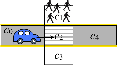
Consider, once again, the autonomous vehicle problem described in Example 1 and Example 2. Suppose the road is discretized into 5 cells c0,…,c4c_{0},\ldots,c_{4} where c2c_{2} is the pedestrian crossing area as shown in Figure 1. The vehicle starts in cell c0c_{0} and has to reach cell c4c_{4}. There are 5 pedestrians, modeled by MCs ℳ1,…,ℳ5{\mathcal{M}}_{1},\ldots,{\mathcal{M}}_{5}, initially at cell c1c_{1}. The models of the vehicle and the pedestrians are shown in Figure 2. A DFA 𝒜φ{\mathcal{A}}_{\varphi} that accepts all and only words in p​r​e​f​(φ)pref(\varphi) where φ=(¬⋁i≥1,j≥0(cj0∧cji))​𝒰​c40\varphi=\left(\neg\bigvee_{i\geq 1,j\geq 0}(c^{0}_{j}\wedge c^{i}_{j})\right)\hskip 2.84526pt\mathcal{U}\hskip 2.84526ptc^{0}_{4} is shown in Figure 3.

Refer to caption
Fig. 1: The road and its partition used in the autonomous vehicle example.
c0c_{0}startc2c_{2}c4c_{4}α1\alpha_{1}α2\alpha_{2}α1\alpha_{1}α2\alpha_{2}α1\alpha_{1}
(a) The vehicle model 𝒯{\mathcal{T}}
c1c_{1}startc2c_{2}c3c_{3}0.60.60.40.40.20.20.80.811
(b) The pedestrian models ℳ1,…,ℳ4{\mathcal{M}}_{1},\ldots,{\mathcal{M}}_{4}
c1c_{1}startc2c_{2}c3c_{3}0.60.60.40.40.20.20.40.40.40.40.60.60.40.4
(c) The pedestrian model ℳ5{\mathcal{M}}_{5}
Fig. 2: The models of vehicle and pedestrians.
q0q_{0}startq1q_{1}q2q_{2}¬c​o​l∧¬c40\neg col\wedge\neg c^{0}_{4}c40c^{0}_{4}c​o​l∧¬c40\hskip-8.53581ptcol\wedge\neg c^{0}_{4}𝑇𝑟𝑢𝑒\mathit{True}𝑇𝑟𝑢𝑒\mathit{True}
Fig. 3: A DFA 𝒜φ{\mathcal{A}}_{\varphi} that recognizes the prefixes of φ=¬c​o​l​𝒰​c40\varphi=\neg col\hskip 2.84526pt\mathcal{U}\hskip 2.84526ptc^{0}_{4} where c​o​lcol is defined as c​o​l=⋁i≥1,j≥0(cj0∧cji)col=\bigvee_{i\geq 1,j\geq 0}(c^{0}_{j}\wedge c^{i}_{j}). q1q_{1} is the accepting state.

First, we apply the LP-based, value iteration and SCC-based value iteration techniques described in Section IV to synthesize a control policy that maximizes the probability that the complete system ℳ=𝒯​‖ℳ1‖​ℳ2​‖…‖​ℳ5{\mathcal{M}}={\mathcal{T}}||{\mathcal{M}}_{1}||{\mathcal{M}}_{2}||\ldots||{\mathcal{M}}_{5} satisfies φ\varphi. The time required for each step of computation is summarized in Table I. All the approaches yield the probability of 0.8 that ℳ{\mathcal{M}} satisfies φ\varphi under the synthesized control policy. The comparison of the total computation time required for these different approaches is shown in Figure 4. As discussed in Section IV-C, although the SCC-based value iteration itself takes significantly less computation time than the LP-based technique or value iteration, the time spent in identifying SCCs and their order renders the total computation time of the SCC-based value iteration more than the other two approaches.

Technique ℳp{\mathcal{M}}_{p} SCCs& orderof ​ℳp\begin{array}[]{c}\hbox{SCCs}\\ \hbox{\& order}\\ \hbox{of }{\mathcal{M}}_{p}\end{array} Probvector\begin{array}[]{c}\hbox{Prob}\\ \hbox{vector}\end{array} Controlpolicy\begin{array}[]{c}\hbox{Control}\\ \hbox{policy}\end{array} Total
LP 156.3 - 8.8 6.8 171.9
Valueiteration\begin{array}[]{c}\hbox{Value}\\ \hbox{iteration}\end{array} 156.3 - 31.3 6.8 194.4
SCC-basedvalue iteration\begin{array}[]{c}\hbox{SCC-based}\\ \hbox{value iteration}\end{array} 156.3 71.1 1.9 6.8 236.1
TABLE I: Time required (in seconds) for computing various objects using different techniques when the full models of all the environment agents are considered.

Next, we apply the incremental technique where we progressively compute a sequence of control policies as more agents are added to the synthesis procedure in each iteration as described in Section V. We let 𝐌0=∅\mathbf{M}_{0}=\emptyset, 𝐌1={ℳ1}\mathbf{M}_{1}=\{{\mathcal{M}}_{1}\}, 𝐌2={ℳ1,ℳ2},…\mathbf{M}_{2}=\{{\mathcal{M}}_{1},{\mathcal{M}}_{2}\},\ldots, 𝐌6={ℳ1,…,ℳ5}\mathbf{M}_{6}=\{{\mathcal{M}}_{1},\ldots,{\mathcal{M}}_{5}\}, i.e., we successively add each pedestrian ℳ1,ℳ2,…,ℳ5{\mathcal{M}}_{1},{\mathcal{M}}_{2},\ldots,{\mathcal{M}}_{5}, respectively, in each iteration. We consider 2 cases: (1) no incremental construction of various objects is employed (i.e., when ℳ𝐌k+1{\mathcal{M}}^{\mathbf{M}_{k+1}} and ℳp𝐌k+1{\mathcal{M}}^{\mathbf{M}_{k+1}}_{p}, k≥0k\geq 0 are computed from scratch in every iteration), and (2) incremental construction of various objects as described in Section V-B–V-D is applied. For the first case, we apply the LP-based technique to compute the probability vector as it has been shown to be the fastest technique when applied to this problem, taking into account the required pre-computation, which needs to be done in every iteration. For both cases, 6 control policies 𝒞𝐌0,…,𝒞𝐌5{\mathcal{C}}^{\mathbf{M}_{0}},\ldots,{\mathcal{C}}^{\mathbf{M}_{5}} are generated for ℳ𝐌0,…,ℳ𝐌5{\mathcal{M}}^{\mathbf{M}_{0}},\ldots,{\mathcal{M}}^{\mathbf{M}_{5}}, respectively. For each policy 𝒞𝐌k{\mathcal{C}}^{\mathbf{M}_{k}}, we compute the probability Prℳ𝒞𝐌k​(φ)\mathrm{Pr}^{{\mathcal{C}}^{\mathbf{M}_{k}}}_{{\mathcal{M}}}(\varphi) that the complete system ℳ{\mathcal{M}} satisfies φ\varphi under policy 𝒞𝐌k{\mathcal{C}}^{\mathbf{M}_{k}}. (Note that 𝒞𝐌k{\mathcal{C}}^{\mathbf{M}_{k}}, when applied to ℳ{\mathcal{M}}, is only a function of states of ℳi∈𝐌k{\mathcal{M}}_{i}\in\mathbf{M}_{k} since it assumes that the other agents ℳj∉𝐌k{\mathcal{M}}_{j}\not\in\mathbf{M}_{k} are stationary.) These probabilities are given by Prℳ𝒞𝐌0​(φ)=0.08\mathrm{Pr}^{{\mathcal{C}}^{\mathbf{M}_{0}}}_{{\mathcal{M}}}(\varphi)=0.08, Prℳ𝒞𝐌1​(φ)=0.46\mathrm{Pr}^{{\mathcal{C}}^{\mathbf{M}_{1}}}_{{\mathcal{M}}}(\varphi)=0.46, Prℳ𝒞𝐌2​(φ)=0.57\mathrm{Pr}^{{\mathcal{C}}^{\mathbf{M}_{2}}}_{{\mathcal{M}}}(\varphi)=0.57, Prℳ𝒞𝐌3​(φ)=0.63\mathrm{Pr}^{{\mathcal{C}}^{\mathbf{M}_{3}}}_{{\mathcal{M}}}(\varphi)=0.63, Prℳ𝒞𝐌4​(φ)=0.67\mathrm{Pr}^{{\mathcal{C}}^{\mathbf{M}_{4}}}_{{\mathcal{M}}}(\varphi)=0.67 and Prℳ𝒞𝐌5​(φ)=0.8\mathrm{Pr}^{{\mathcal{C}}^{\mathbf{M}_{5}}}_{{\mathcal{M}}}(\varphi)=0.8.

The comparison of the cases where the incremental construction of various objects is not and is employed is shown in Figure 4. A jump in the probability occurs each time a new control policy is computed. The time spent during each step of computation is summarized in Table II and Table III for the first and the second case, respectively. Notice that the time required for identifying the SCCs and their order when the incremental approach is applied is significantly less than when the full model of all the pedestrians is considered in one shot since ℳ𝐌0{\mathcal{M}}^{\mathbf{M}_{0}}, ℳ1,…,ℳ5{\mathcal{M}}_{1},\ldots,{\mathcal{M}}_{5}, each of which contains 3 states, are much smaller than ℳp{\mathcal{M}}_{p}, which contains 2187 states.

Fig. 4: Comparison of the computation time and the probability for the system to satisfy the specification computed using different techniques.

From Figure 4, our incremental approach is able to obtain an optimal control policy faster than any other techniques. This is mainly due to the efficiency of our incremental construction of SCCs and their order. In addition, we are able to obtain a reasonable solution, with 0.67 probability of satisfying φ\varphi, within 12 seconds while the maximum probability of satisfying φ\varphi is 0.8, which requires 160 seconds of computation (or 171.9 seconds without employing the incremental approach).

Iteration ℳ𝐌k{\mathcal{M}}^{\mathbf{M}_{k}} ℳp𝐌k{\mathcal{M}}^{\mathbf{M}_{k}}_{p} Probvector\begin{array}[]{c}\hbox{Prob}\\ \hbox{vector}\end{array} Controlpolicy\begin{array}[]{c}\hbox{Control}\\ \hbox{policy}\end{array} Total
0 0.0064 0.0185 0.0464 0.0084 0.08
1 0.0123 0.0762 0.0203 0.0104 0.12
2 0.0154 0.3383 0.0231 0.0296 0.41
3 0.0357 1.7055 0.0542 0.1503 1.95
4 0.1393 9.1950 0.2155 0.7975 10.35
5 3.1836 152.86 8.2302 6.8938 171.17
TABLE II: Time required (in seconds) for computing various objects in each iteration when incremental construction is not applied.
Iter-ation\begin{array}[]{c}\hbox{Iter-}\\ \hbox{ation}\end{array} ℳ𝐌0{\mathcal{M}}^{\mathbf{M}_{0}} SCCs & orderof ​ℳ𝐌0,ℳ1,…,ℳ5\begin{array}[]{c}\hbox{SCCs \& order}\\ \hbox{of }{\mathcal{M}}^{\mathbf{M}_{0}},\\ {\mathcal{M}}_{1},\ldots,{\mathcal{M}}_{5}\end{array} ℳp𝐌k,partition& order\begin{array}[]{c}{\mathcal{M}}^{\mathbf{M}_{k}}_{p},\\ \hbox{partition}\\ \hbox{\& order}\end{array} Probvector\begin{array}[]{c}\hbox{Prob}\\ \hbox{vector}\end{array} Controlpolicy\begin{array}[]{c}\hbox{Control}\\ \hbox{policy}\end{array} Total
0 0.0055 0.0043 0.0203 0.0112 0.0036 0.04
1 - - 0.0726 0.0102 0.0087 0.09
2 - - 0.3239 0.0193 0.0282 0.37
3 - - 1.6036 0.0567 0.1424 1.80
4 - - 8.6955 0.1876 0.7755 9.66
5 - - 139.27 1.6122 7.0125 147.89
TABLE III: Time required (in seconds) for computing various objects in each iteration when incremental construction is applied.

VII Conclusions and Future Work

An anytime algorithm for synthesizing a control policy for a robot interacting with multiple environment agents with the objective of maximizing the probability for the robot to satisfy a given temporal logic specification was proposed. Each environment agent is modeled by a Markov chain whereas the robot is modeled by a finite transition system (in the deterministic case) or Markov decision process (in the stochastic case). The proposed algorithm progressively computes a sequence of control policies, taking into account only a small subset of the environment agents initially and successively adding more agents to the synthesis procedure in each iteration until we hit the constraints on computational resources. Incremental construction of various objects needed to be computed during the synthesis procedure was proposed. Experimental results showed that not only we obtain a reasonable solution much faster than existing approaches, but we are also able to obtain an optimal solution faster than existing approaches.

Future work includes extending the algorithm to handle full LTL specifications. This direction appears to be promising because the remaining step is only to incrementally construct accepting maximal end components of an MDP. We are also examining an effective approach to determine an agent to be added in each iteration. As mentioned in Section V-A, such an agent may be picked based on the result from probabilistic verification but this comes at the extra cost of adding the verification phase.

References

  • [1] E. A. Emerson, “Temporal and modal logic,” Handbook of Theoretical Computer Science (Vol. B): Formal Models and Semantics, pp. 995–1072, 1990.
  • [2] Z. Manna and A. Pnueli, The temporal logic of reactive and concurrent systems. Springer-Verlag, 1992.
  • [3] C. Baier and J.-P. Katoen, Principles of Model Checking (Representation and Mind Series). The MIT Press, 2008.
  • [4] G. Fainekos, H. Kress-Gazit, and G. Pappas, “Temporal logic motion planning for mobile robots,” in IEEE International Conference on Robotics and Automation, pp. 2020–2025, 2005.
  • [5] H. Kress-Gazit, G. Fainekos, and G. Pappas, “Where’s Waldo? Sensor-based temporal logic motion planning,” in IEEE International Conference on Robotics and Automation, pp. 3116–3121, 2007.
  • [6] C. Belta, A. Bicchi, M. Egerstedt, E. Frazzoli, E. Klavins, and G. Pappas, “Symbolic planning and control of robot motion [grand challenges of robotics],” IEEE Robotics & Automation Magazine, vol. 14, no. 1, pp. 61–70, 2007.
  • [7] D. Conner, H. Kress-Gazit, H. Choset, A. Rizzi, and G. Pappas, “Valet parking without a valet,” in IEEE/RSJ International Conference on Intelligent Robots and Systems, 2007, pp. 572–577, 2007.
  • [8] S. Karaman and E. Frazzoli, “Sampling-based motion planning with deterministic μ\mu-calculus specifications,” in Proc. of IEEE Conference on Decision and Control, 2009.
  • [9] A. Bhatia, L. E. Kavraki, and M. Y. Vardi, “Sampling-based motion planning with temporal goals,” in IEEE International Conference on Robotics and Automation (ICRA), pp. 2689–2696, 2010.
  • [10] X. C. Ding, S. L. Smith, C. Belta, and D. Rus, “LTL control in uncertain environments with probabilistic satisfaction guarantees,” in IFAC World Congress, 2011.
  • [11] A. I. Medina Ayala, S. B. Andersson, and C. Belta, “Temporal logic control in dynamic environments with probabilistic satisfaction guarantees,” in IEEE/RSJ International Conference on Intelligent Robots and Systems, 2007, pp. 3108–3113, 2011.
  • [12] H. Kress-Gazit, T. Wongpiromsarn, and U. Topcu, “Correct, reactive robot control from abstraction and temporal logic specifications,” Special Issue of the IEEE Robotics & Automation Magazine on Formal Methods for Robotics and Automation, vol. 18, pp. 65–74, 2011.
  • [13] O. Kupferman and M. Y. Vardi, “Model checking of safety properties,” Formal Methods in System Design, vol. 19, pp. 291–314, 2001.
  • [14] T. Latvala, “Efficient model checking of safety properties,” in Model Checking Software. 10th International SPIN Workshop, pp. 74–88, Springer, 2003.
  • [15] F. Ciesinski, C. Baier, M. Größer, and J. Klein, “Reduction techniques for model checking markov decision processes,” in Proceedings of the 2008 Fifth International Conference on Quantitative Evaluation of Systems, pp. 45–54, 2008.
  • [16] M. Kwiatkowska, D. Parker, and H. Qu, “Incremental quantitative verification for markov decision processes,” in IEEE/IFIP International Conference on Dependable Systems & Networks, pp. 359–370, 2011.
  • [17] R. Tarjan, “Depth-first search and linear graph algorithms,” SIAM Journal on Computing, vol. 1, pp. 146–160, 1972.