Control of Probabilistic Systems under Dynamic, Partially Known Environments with Temporal Logic Specifications
Abstract
We consider the synthesis of control policies for probabilistic systems, modeled by Markov decision processes, operating in partially known environments with temporal logic specifications. The environment is modeled by a set of Markov chains. Each Markov chain describes the behavior of the environment in each mode. The mode of the environment, however, is not known to the system. Two control objectives are considered: maximizing the expected probability and maximizing the worst-case probability that the system satisfies a given specification.
I Introduction
In many applications, control systems need to perform complex tasks and interact with their (potentially adversarial) environments. The correctness of these systems typically depends on the behaviors of the environments. For example, whether an autonomous vehicle exhibits a correct behavior at a pedestrian crossing depends on the behavior of the pedestrians, e.g., whether they actually cross the road, remain on the same side of the road or step in front of the vehicle while it is moving.
Temporal logics, which were primarily developed by the formal methods community for specifying and verifying correctness of software and hardware systems, have been recently employed to express complex behaviors of control systems. Its expressive power offers extensions to properties that can be expressed than safety and stability, typically studied in the control and hybrid systems domains. In particular, [1] shows that the traffic rule enforced in the 2007 DARPA Urban Challenge can be precisely described using these logics. Furthermore, the recent development of language equivalence and simulation notions allows abstraction of continuous systems to a purely discrete model [2, 3, 4]. This subsequently provides a framework for integrating methodologies from the formal methods and the control-theoretic communities and enables formal specification, design and verification of control systems with complex behaviors.
Controller synthesis from temporal logic specifications has been considered in [5, 6, 7, 8], assuming static environments. Synthesis of reactive controllers that takes into account all the possible behaviors of dynamic environments can be found in [9, 10]. In this case, the environment is treated as an adversary and the synthesis problem can be viewed as a two-player game between the system and the environment: the environment attempts to falsify the specification while the system attempts to satisfy it [11]. In these works, the system is assumed to be deterministic, i.e., an available control action in each state enables exactly one transition. Controller synthesis for probabilistic systems such as Markov decision processes (MDP) has been considered in [12, 13]. However, these works assume that at any time instance, the state of the system, including the environment, as well as their models are fully known. This may not be a valid assumption in many applications. For example, in the pedestrian crossing problem previously described, the behavior of the pedestrians depend on their destination, which is typically not known to the system. Having to account for all the possible behaviors of the pedestrians with respect to all their possible destinations may lead to conservative results and in many cases, unrealizable specifications.
Partially observable Markov decision process (POMDP) provides a principled mathematical framework to cope with partial observability in stochastic domains [14]. Roughly, the main idea is to maintain a belief, which is defined as a probability distribution over all the possible states. POMDP algorithms then operate in the belief space. Unfortunately, it has been shown that solving POMDPs exactly is computationally intractable [15]. Hence, point-based algorithms have been developed to compute an approximate solution based on the computation over a representative set of points from the belief space rather than the entire belief space [16].
In this paper, we take an initial step towards solving POMDPs that are subject to temporal logic specifications. In particular, we consider the problem where a collection of possible environment models is available to the system. Different models correspond to different modes of the environment. However, the system does not know in which mode the environment is. In addition, the environment may change its mode during an execution subject to certain constraints. We consider two control objectives: maximizing the expected probability and maximizing the worst-case probability that the system satisfies a given temporal logic specification. The first objective is closely related to solving POMDPs as previously described whereas the second objective is closely related to solving uncertain MDPs [17]. However, for both problems, we aim at maximizing the expected or worst-case probability of satisfying a temporal logic specification, instead of maximizing the expected or worst-case reward as considered in the POMDP and MDP literature.
The main contribution of this paper is twofold. First, we show that the expectation-based synthesis problem can be formulated as a control policy synthesis problem for MDPs under temporal logic specifications and provide a complete solution to the problem. Second, we define a mathematical object called adversarial Markov decision process (AMDP) and show that the worst-case-based synthesis problem can be formulated as a control policy synthesis problem for AMDP. A complete solution to the control policy synthesis for AMDP is then provided. Finally, we show that the maximum worst-case probability that a given specification is satisfied does not depend on whether the controller and the adversary play alternatively or both the control and adversarial policies are computed at the beginning of an execution.
The rest of the paper is organized as follows: We provide useful definitions and descriptions of the formalisms in the following section. Section III is dedicated to the problem formulation. The expectation-based and the worst-case-based control policy synthesis are considered in Section IV and Section V, respectively. Section VI presents an example. Finally, Section VII concludes the paper and discusses future work.
II Preliminaries
We consider systems that comprise stochastic components. In this section, we define the formalisms used in this paper to describe such systems and their desired properties. Throughout the paper, we let , and denote the set of finite, infinite and nonempty finite strings, respectively, of a set .
II-A Automata
Definition 1
A deterministic Rabin automaton (DRA) is a tuple where
- •
is a finite set of states,
- •
is a finite set called alphabet,
- •
is a transition function,
- •
is the initial state, and
- •
is the acceptance condition.
We use the relation notation, to denote .
Consider an infinite string . A run for in a DRA is an infinite sequence of states such that and for all . A run is accepting if there exists a pair such that (1) there exists such that for all , , and (2) there exist infinitely many such that .
A string is accepted by if there is an accepting run of in . The language accepted by , denoted by , is the set of all accepted strings of .
II-B Linear Temporal Logic
Linear temporal logic (LTL) is a branch of logic that can be used to reason about a time line. An LTL formula is built up from a set of atomic propositions, the logic connectives , , and and the temporal modal operators (“next”), (“always”), (“eventually”) and (“until”). An LTL formula over a set of atomic propositions is inductively defined as
where . Other operators can be defined as follows: , , , and .
Semantics of LTL: LTL formulas are interpreted on infinite strings over . Let where for all . The satisfaction relation is defined inductively on LTL formulas as follows:
- •
,
- •
for an atomic proposition , if and only if ,
- •
if and only if ,
- •
if and only if and ,
- •
if and only if , and
- •
if and only if there exists such that and for all such all , .
Given propositional formulas and , examples of widely used LTL formulas include a safety formula (read as “always ”), which simply asserts that property remains invariantly true throughout an execution and a reachability formula (read as “eventually ”), which states that property becomes true at least once in an execution (i.e., there exists a reachable state that satisfies ). In the example presented later in this paper, we use a formula (read as “ until ”), which asserts that has to remain true until becomes true and there is some point in an execution where becomes true.
II-C Systems and Control Policies
Definition 2
A (discrete-time) Markov chain (MC) is a tuple where
- •
is a countable set of states,
- •
is the transition probability function such that for any state , ,
- •
is the initial state,
- •
is a set of atomic propositions, and
- •
is a labeling function.
Definition 3
A Markov decision process (MDP) is a tuple where , , and are defined as in MC and
- •
is a finite set of actions, and
- •
is the transition probability function such that for any state and action ,
An action is enabled in state if and only if . Let denote the set of enabled actions in .
Given a complete system as the composition of all its components, we are interested in computing a control policy for the system that optimizes certain objectives. We define a control policy for a system modeled by an MDP as follows.
Definition 4
Let be a Markov decision process. A control policy for is a function such that for all .
Let be an MDP and be a control policy for . An infinite sequence on generated under policy is called a path on if and for all . The subsequence where is the prefix of length of . We define and as the set of all infinite paths of under policy and their finite prefixes, respectively. For , we let denote the set of all paths in with prefix .
The -algebra associated with under policy is defined as the smallest -algebra that contains where ranges over all finite paths in . It follows that there exists a unique probability measure on the algebra associated with under policy where for any ,
| (1) |
Given an LTL formula , one can show that the set is measurable [19]. The probability for to satisfy under policy is then defined as
For a given (possibly noninitial) state , we let , i.e., is the same as except that its initial state is . We define as the probability for to satisfy under policy , starting from .
A control policy essentially resolves all the nondeterministic choices in an MDP and induces a Markov chain that formalizes the behavior of under control policy [19]. In general, contains all the states in and hence may not be finite even though is finite. However, for a special case where is a memoryless or a finite memory control policy, it can be shown that can be identified with a finite MC. Roughly, a memoryless control policy always picks the action based only on the current state of , regardless of the path that led to that state. In contrast, a finite memory control policy also maintains its “mode” and picks the action based on its current mode and the current state of .
III Problem Formulation
Consider a system that comprises 2 components: the plant and the environment. The system can regulate the state of the plant but has no control over the state of the environment. We assume that at any time instance, the state of the plant and the environment can be precisely observed.
The plant is modeled by a finite MDP . We assume that for each , there is an action that is enabled in state . In addition, we assume that the environment can be modeled by some MC in where for each , is a finite MC that represents a possible model of the environment. For the simplicity of the presentation, we assume that for all , , , and ; hence, differ only in the transition probability function. These different environment models can be considered as different modes of the environment. For the rest of the paper, we use “environment model” and “environment mode” interchangeably to refer to some .
We further assume that the plant and the environment make a transition simultaneously, i.e., both of them makes a transition at every time step. All are available to the system. However, the system does not know exactly which is the actual model of the environment. Instead, it maintains the belief , which is defined as a probability distribution over all possible environment models such that . returns the probability that is the model being executed by the environment. The set of all the beliefs forms the belief space, which we denote by . In order to obtain the belief at each time step, the system is given the initial belief . Then, it subsequently updates the belief using a given belief update function such that returns the belief after the environment makes a transition from state with belief to state . The belief update function can be defined based on the observation function as in the belief MDP construction for POMDPs [14].
In general, the belief space may be infinite, rendering the control policy synthesis computationally intractable to solve exactly. To overcome this difficulty, we employ techniques for solving POMDPs and approximate by a finite set of representative points from and work with this approximate representation instead. Belief space approximation is beyond the scope of this paper and is subject to future work. Sampling techniques that have been proposed in the POMDP literature can be found in, e.g., [16, 22, 23].
Given a system model described by , , the (finite) belief space , the initial belief , the belief update function and an LTL formula that describes the desired property of the system, we consider the following control policy synthesis problems.
Problem 1
Synthesize a control policy for the system that maximizes the expected probability that the system satisfies where the expected probability that the environment transitions from state with belief to state is given by .
Problem 2
Synthesize a control policy for the system that maximizes the worst-case (among all the possible sequences of environment modes) probability that the system satisfies . The environment mode may change during an execution: when the environment is in state with belief , it may switch to any mode with . We consider both the case where the controller and the environment plays a sequential game and the case where the control policy and the sequence of environment modes are computed before an execution.
Example 1
Consider a problem where an autonomous vehicle needs to navigate a road with a pedestrian walking on the pavement. The vehicle and the pedestrian are considered the plant and the environment, respectively. The pedestrian may or may not cross the road, depending on his/her destination, which is unknown to the system. Suppose the road is discretized into a finite number of cells . The vehicle is modeled by an MDP whose state describes the cell occupied by the vehicle and whose action corresponds to a motion primitive of the vehicle (e.g., cruise, accelerate, decelerate). The motion of the pedestrian is modeled by an MC where . represents the model of the pedestrian if s/he decides not to cross the road whereas represents the model of the pedestrian if s/he decides to cross the road. A state describes the cell occupied by the pedestrian. The labeling functions and essentially maps each cell to its label, with an index that identifies the vehicle from the pedestrian, i.e., and for all . Consider the desired property stating that the vehicle does not collide with the pedestrian until it reaches cell (e.g., the end of the road). In this case, the specification can be written as .
IV Expectation-Based Control Policy Synthesis
To solve Problem 1, we first construct the MDP that represents the complete system, taking into account the uncertainties, captured by the belief, in the environment model. Then, we employ existing results in probabilistic verification and construct the product MDP and extract its optimal control policy. In this section, we describe these steps in more detail and discuss their connection to Problem 1.
IV-A Construction of the Complete System
Based on the notion of belief, we construct the complete environment model, represented by the MC where for each and ,
| (2) |
and .
It is straightforward to check that for all , . Hence, is a valid MC.
Assuming that the plant and the environment make a transition simultaneously, we obtain the complete system by constructing the synchronous parallel composition of the plant and the environment. Synchronous parallel composition of MDP and MC is defined as follows.
Definition 5
Let be a Markov decision process and be a Markov chain. Their synchronous parallel composition, denoted by , is the MDP where:
- •
For each , and , .
- •
For each and , .
From the above definitions, our complete system can be modeled by the MDP . We denote this MDP by . Note that a state is of the form where , and . The following lemma shows that Problem 1 can be solved by finding a control policy for that maximizes .
Lemma 1
Let be a finite path of under policy where for each , . Then,
| (3) |
Hence, given an LTL formula , gives the expected probability that the system satisfies under policy .
Proof:
The proof straightforwardly follows from the definition of and . ∎
IV-B Construction of the Product MDP
Let be a DRA that recognizes the specification . Our next step is to obtain a finite MDP as the product of and , defined as follows.
Definition 6
Let be an MDP and let be a DRA. Then, the product of and is the MDP defined by where , , , and
| (4) |
Consider a path of under some control policy . We say that is accepting if and only if there exists a pair such that the word generated by intersects with finitely many times and intersects with infinitely many times, i.e., (1) there exists such that for all , , and (2) there exists infinitely many such that .
Stepping through the above definition shows that given a path of generated under some control policy , the corresponding path on generates a word that satisfies if and only if is accepting. Therefore, each accepting path of uniquely corresponds to a path of whose word satisfies . In addition, a control policy on induces a corresponding control policy on . The details for generating from can be found, e.g., in [19, 12].
IV-C Control Policy Synthesis for Product MDP
From probabilistic verification, it has been shown that the maximum probability for to satisfy is equivalent to the maximum probability of reaching a certain set of states of known as accepting maximal end components (AMECs). An end component of the product MDP is a pair where and such that (1) for all , (2) the directed graph induced by is strongly connected, and (3) for all and , . An accepting maximal end component of is an end component such that for some , and and there is no end component such that and for all . It has an important property that starting from any state in , there exists a finite memory control policy to keep the state within forever while visiting all states in infinitely often with probability 1. AMECs of can be efficiently identified based on iterative computations of strongly connected components of . We refer the reader to [19] for more details.
Once the AMECs of are identified, we then compute the maximum probability of reaching where contains all the states in the AMECs of . For the rest of the paper, we use an LTL-like notations to describe events in MDPs. In particular, we use to denote the event of reaching some state in eventually.
For each , let denote the maximum probability of reaching a state in , starting from . Formall, . There are two main techniques for computing the probability for each : linear programming (LP) and value iteration. LP-based techniques yield an exact solution but it typically does not scale as well as value iteration. On the other hand, value iteration is an iterative numerical technique. This method works by successively computing the probability vector for increasing such that for all . Initially, we set if and otherwise. In the th iteration where , we set
| (5) |
In practice, we terminate the computation and say that converges when a termination criterion such as is satisfied for some fixed (typically very small) threshold .
Once the vector is computed, a finite memory control policy for that maximizes the probability for to satisfy can be constructed as follows. First, consider the case when is in state . In this case, belongs to some AMEC and the policy selects an action such that all actions in are scheduled infinitely often. (For example, may select the action for according to a round-robin policy.) Next, consider the case when is in state . In this case, picks an action to ensure that can be achieved. If , an action in can be chosen arbitrarily. Otherwise, picks an action such that for some with . Here, is the set of actions such that for all , and denotes the length of a shortest path from to a state in , using only actions in .
V Worst-Case-Based Control Policy Synthesis
To solve Problem 2, we first propose a mathematical object called adversarial Markov decision process (AMDP). Then, we show that Problem 2 can be formulated as finding an optimal control policy for an AMDP. Finally, control policy synthesis for AMDP is discussed.
V-A Adversarial Markov Decision Process
Definition 7
An adversarial Markov decision process (AMDP) is a tuple where , , and are defined as in MDP and
- •
is a finite set of control actions,
- •
is a finite set of adversarial actions, and
- •
is the transition probability function such that for any , and , .
We say that a control action is enabled in state if and only if there exists an adversarial action such that . Similarly, an adversarial action is enabled in state if and only if there exists a control action such that . Let and denote the set of enabled control and adversarial actions, respectively, in . We assume that for all , and , , i.e., whether an adversarial (resp. control) action is enabled in state depends only on the state itself but not on a control (resp. adversarial) action taken by the system (resp. adversary).
Given an AMDP , a control policy and an adversarial policy for an AMDP can be defined such that and for all . A unique policy measure on the -algebra associated with under control policy and adversarial policy can then be defined based on the notion of path on as for an ordinary MDP.
We end the section with important properties of AMDP that will be employed in the control policy synthesis.
Definition 8
Let be a set of functions from to where and are finite sets. We say that is complete if for any and , there exists such that and .
Lemma 2
Let , and be finite sets and let be a set of functions from to . Then, is finite. Furthermore, suppose that is complete. Then, for any and ,
| (6) |
In addition,
| (7) |
Proof:
Since both and are finite, clearly, is finite. Thus, the and in (6)–(7) are well defined. Let be a function such that . Since is complete, there exists a function such that for all , satisfies . Furthermore, since both and are non-negative and , it follows that for all and . Taking the sum over all , we get
| (8) |
But since , it follows that
| (9) |
Combining (8) and (9), we get that all the inequalities must be replaced by equalities. Hence, we can conclude that the first equality in (6) holds. The proof for the equality in (7) follows similar arguments. Hence, we only provide a proof for the second inequality in (6).
First, from weak duality, we know that
| (10) |
For each , consider an element such that . Since , it follows that
| (11) |
But, from the definition of and and the first equality in (6), we also get
| (12) |
Following the chain of inequalities in (10)–(12), we can conclude that the second equality in (6) holds. ∎
Proposition 1
Let , be a finite AMDP and be the set of goal states. Let
| (13) |
where for any , , , and . For each , consider a vector where for all , for all and for all ,
| (14) |
Then, for any , and .
Proof:
Since for all and , it can be checked that for any , if for all , then for all . Since, for all , we can conclude that for all and .
Let denote the event of reaching some state in within steps. We will show, using induction on , that for any and ,
| (15) |
where and are control and adversarial policies such that for any such that , and . The case where is trivial so we only consider an arbitrary . Clearly, for any control and adversarial policies and . Consider an arbitrary and assume that for all , (15) holds. Then, from (14), we get that for any ,
Since for all such that , , and are finite, it follows that and are finite. Furthermore, only depends on , , . Thus, we can conclude that all the and above can be attained, so we can replace them by and , respectively.
Consider arbitrary and . Define a function such that . In addition, define a set and a function such that where for any , and . Pick arbitrary and . Suppose and . Then, from the definition of , and ; hence, there must exists such that and . Thus, by definition, is complete. Applying Lemma 2, we get
Applying a similar procedure as in the previous paragraph times, we get
Thus, we can conclude that for any and , (15) holds. Furthermore, since the set of events includes the set of events , we obtain . Finally, we can conclude that using the fact that the sequence is monotonic and bounded (and hence has a finite limit) and is the countable union of the events . ∎
Proposition 2
Let , be a finite AMDP and be the set of goal states. Let
| (16) |
For each , consider a vector where for all , for all and for all ,
| (17) |
Then, for any , and .
Proof:
The proof closely follows the proof of Proposition 1. Roughly, we show, by induction on and applying Lemma 2, that for any and , . We can conclude the proof using a similar argument as in the proof of Proposition 1. ∎
From Proposition 1 and Proposition 2, we can conclude that the sequential game (13) is equivalent to its nonsequential counterpart (16).
Corollary 1
The maximum worst-case probability of reaching a set of states in an AMDP does not depend on whether the controller and the adversary play alternatively or both the control and adversarial policies are computed at the beginning of an execution.
V-B The Complete System as an AMDP
We start by constructing an MDP that represents the complete system as described in Section IV-A. As discussed earlier, a state of is of the form where , and . The corresponding AMDP of is then defined as where , (i.e., corresponds to the environment choosing model and for any , , , and ,
| (18) |
if ; otherwise, .
It is straightforward to check that is a valid AMDP. Furthermore, based on this construction and the assumptions that (1) at any plant state , there exists an action that is enabled in , and (2) at any point in an execution, the belief satisfies , it can be shown that at any state , there exists a control action and an adversarial action that are enabled in . In addition, consider the case where the environment is in state with belief . It can be shown that for all , if , then is enabled in for all . Thus, we can conclude that represents the complete system for Problem 2.
Remark 1
According to (18), the system does not need to maintain the exact belief in each state. The only information needed to construct an AMDP that represents the complete system is all the possible modes of the environment in each state of the complete system. This allows us to integrate methodologies for discrete state estimation [24] to reduce the size of the AMDP. This direction is subject to future work.
V-C Control Policy Synthesis for AMDP
Similar to control policy synthesis for MDP, control policy synthesis for AMDP can be done on the basis of a product construction. The product of and DRA is an AMDP , which is defined similar to the product of MDP and DRA, except that the set of actions is partitioned into the set of control and the set of adversarial actions.
Following the steps for synthesizing a control policy for product MDP, we identify the AMECs of . An AMEC of is defined based on the notion of end component as for the case of product MDP. However, an end component of needs to be defined, taking into account the adversary. Specifically, an end component of is a pair where and such that (1) for all , (2) the directed graph induced by under any adversarial policy is strongly connected, and (3) for all , and , .
Using a similar argument as in the case of product MDP [19], it can be shown that the maximum worst-case probability for to satisfy is equivalent to the maximum worst-case probability of reaching a states in an AMEC of . We can then apply Proposition 1 and Proposition 2 to compute , which is equivalent to , using value iteration. A control policy for that maximizes the worst-case probability for to satisfy can be constructed as outlined at the end of Section IV-C for product MDP.
VI Example
Consider, once again, the autonomous vehicle problem described in Example 1. Suppose the road is discretized into 9 cells as shown in Figure 1. The vehicle starts in cell and has to reach cell whereas the pedestrian starts in cell . The models of the vehicle and the pedestrian are shown in Figure 2. The vehicle has two actions and , which correspond to decelerating and accelerating, respectively. The pedestrian has 2 modes and , which correspond to the cases where s/he wants to remain on the left side of the road and cross the road, respectively. A DRA that accepts all and only words that satisfy is shown in Figure 3. Finally, we consider the set of beliefs where for all , and . We set where it is equally likely that the pedestrian is in mode or mode . The belief update function is defined such that the longer the pedestrian stay on the left side of the road, the probability that s/he is in mode increases. Once the pedestrian starts crossing the road, we change the belief to where it is certain that the pedestrian is in mode . Specifically, for all , we let
| (19) |
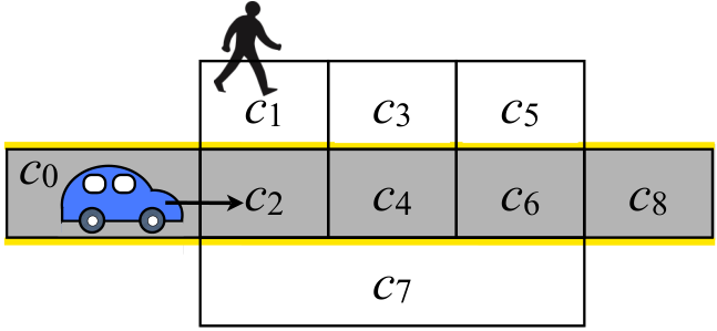
Both the expectation-based and the worst-case-base control policy synthesis as described in Section IV and V is implemented in MATLAB. The computation was performed on a MacBook Pro with a 2.8 GHz Intel Core 2 Duo processor.
First, we consider the expectation-based control policy synthesis (i.e., Problem 1). As outlined in Section IV, we first construct the MDP that represents the complete system. After removing all the unreachable states, the resulting MDP contains 65 states and the product MDP contains 53 states. The computation time is summarized in Table I. Note that the computation, especially the product MDP construction, can be sped up significantly if a more efficient representation of DRA is used. The maximum expected probability for the system to satisfy is 0.9454. Examination of the resulting control policy shows that this maximum expected probability of satisfying can be achieved by applying action , i.e., decelerating, until the pedestrian crosses the street or the vehicle is not behind the pedestrian in the longitudinal direction, i.e., when the vehicle is in cell and the pedestrian is in cell where . (Based on the expectation, the probability that the pedestrian eventually crosses the road is 1 according to the probability measure defined in (1).) If we include the belief where and , then the expectation-based optimal control policy is such that the vehicle applies until either the pedestrian crosses the road, the vehicle is not behind the pedestrian in the longitudinal direction or the belief is updated to , at which point, it applies . Once the vehicle reaches the destination , it applies forever.
Next, we consider the worst-case-based control policy synthesis (i.e., Problem 2). In this case, the resulting AMDP contains 49 states and the product AMDP contains 53 states after removing all the unreachable states. The maximum worst-case probability for the system to satisfy is 0.9033. The resulting control policy is slightly more aggressive than the expectation-based policy. In addition to the cases where the expectation-based controller applies , the worst-case-based controller also applies when the vehicle is in and the pedestrian is in and when the vehicle is in and the pedestrian is in .
| Total | |||||
|---|---|---|---|---|---|
| Expectation | 0.05 | 2.31 | 0.73 | 0.08 | 3.17 |
| Worst-case | 0.20 | 2.73 | 0.46 | 0.05 | 3.44 |
Simulation results are shown in Figure 4 and Figure 5. The smaller (red) rectangle represents the pedestrian whereas the bigger (blue) rectangle represents the vehicle. The filled and unfilled rectangles represent their current positions and the trace of their trajectories, respectively. Notice that the vehicle successfully reaches its goal without colliding with the pedestrian, as required by its specification, with the worst-case-based controller being slightly more aggressive.
Finally, we would like to note that due to the structure of this example, the worst-case-based synthesis problem can be solved without having to deal with the belief space at all. As the environment cannot be in state , , or when it is in mode and these states only have transitions among themselves, once the environment transitions to one of these states, we know for sure that it can only be in mode and cannot change its mode anymore. In states , and , the environment can be in either mode. Based on this structure and Remark 1, we can construct an AMDP that represents the complete system with smaller number of states than constructed using the method described in Section V-B. Exploiting the structure of the problem to reduce the size of AMDP is subject to future work.
VII Conclusions and Future Work
We took an initial step towards solving POMDPs that are subject to temporal logic specifications. In particular, we considered the problem where the system interacts with its dynamic environment. A collection of possible environment models are available to the system. Different models correspond to different modes of the environment. However, the system does not know in which mode the environment is. In addition, the environment may change its mode during an execution. Control policy synthesis was considered with respect to two different objectives: maximizing the expected probability and maximizing the worst-case probability that the system satisfies a given temporal logic specification.
Future work includes investigating methodologies to approximate the belief space with a finite set of representative points. This problem has been considered extensively in the POMDP literature. Since the value iteration used to obtain a solution to our expectation-based synthesis problem is similar to the value iteration used to solve POMDP problems where the expected reward is to be maximized, we believe that existing sampling techniques used to solve POMDP problems can be adapted to solve our problem. Another direction of research is to integrate methodologies for discrete state estimation to reduce the size of AMDP for the worst-case-based synthesis problem.
Acknowledgments
The authors gratefully acknowledge Tirthankar Bandyopadhyay for inspiring discussions.
References
- [1] T. Wongpiromsarn, S. Karaman, and E. Frazzoli, “Synthesis of provably correct controllers for autonomous vehicles in urban environments,” in IEEE Intelligent Transportation Systems Conference, 2011.
- [2] R. Alur, T. A. Henzinger, G. Lafferriere, and G. J. Pappas, “Discrete abstractions of hybrid systems,” Proc. of the IEEE, vol. 88, no. 7, pp. 971–984, 2000.
- [3] H. Tanner and G. J. Pappas, “Simulation relations for discrete-time linear systems,” in Proc. of the IFAC World Congress on Automatic Control, pp. 1302–1307, 2002.
- [4] A. Girard and G. J. Pappas, “Hierarchical control system design using approximate simulation,” Automatica, vol. 45, no. 2, pp. 566–571, 2009.
- [5] P. Tabuada and G. J. Pappas, “Linear time logic control of linear systems,” IEEE Transaction on Automatic Control, vol. 51, no. 12, pp. 1862–1877, 2006.
- [6] M. Kloetzer and C. Belta, “A fully automated framework for control of linear systems from temporal logic specifications,” IEEE Transaction on Automatic Control, vol. 53, no. 1, pp. 287–297, 2008.
- [7] S. Karaman and E. Frazzoli, “Sampling-based motion planning with deterministic -calculus specifications,” in Proc. of IEEE Conference on Decision and Control, 2009.
- [8] A. Bhatia, L. E. Kavraki, and M. Y. Vardi, “Sampling-based motion planning with temporal goals,” in IEEE International Conference on Robotics and Automation (ICRA), pp. 2689–2696, 2010.
- [9] H. Kress-Gazit, G. E. Fainekos, and G. J. Pappas, “Temporal logic-based reactive mission and motion planning,” IEEE Transactions on Robotics, vol. 25, no. 6, pp. 1370–1381, 2009.
- [10] T. Wongpiromsarn, U. Topcu, and R. M. Murray, “Receding horizon control for temporal logic specifications,” in Hybrid Systems: Computation and Control, 2010.
- [11] N. Piterman, A. Pnueli, and Y. Sa’ar, “Synthesis of reactive(1) designs,” in Verification, Model Checking and Abstract Interpretation, vol. 3855 of Lecture Notes in Computer Science, pp. 364 – 380, Springer-Verlag, 2006.
- [12] X. C. Ding, S. L. Smith, C. Belta, and D. Rus, “LTL control in uncertain environments with probabilistic satisfaction guarantees,” in IFAC World Congress, 2011.
- [13] X. C. Ding, S. L. Smith, C. Belta, and D. Rus, “Mdp optimal control under temporal logic constraints,” in Proc. of IEEE Conference on Decision and Control, 2011.
- [14] L. P. Kaelbling, M. L. Littman, and A. R. Cassandra, “Planning and acting in partially observable stochastic domains,” Artificial Intelligence, vol. 101, pp. 99–134, 1998.
- [15] C. Papadimitriou and J. N. Tsitsiklis, “The complexity of markov decision processes,” Mathematics of Operations Research, vol. 12, pp. 441–450, 1987.
- [16] M. Hauskrecht, “Value-function approximations for partially observable markov decision processes,” Journal of Artificial Intelligence Research, vol. 13, pp. 33–94, 2000.
- [17] A. Nilim and L. El Ghaoui, “Robust control of markov decision processes with uncertain transition matrices,” Operations Research, vol. 53, pp. 780–798, 2005.
- [18] J. Klein and C. Baier, “Experiments with deterministic -automata for formulas of linear temporal logic,” Theoretical Computer Science, vol. 363, pp. 182–195, 2006.
- [19] C. Baier and J.-P. Katoen, Principles of Model Checking (Representation and Mind Series). The MIT Press, 2008.
- [20] E. A. Emerson, “Temporal and modal logic,” Handbook of Theoretical Computer Science (Vol. B): Formal Models and Semantics, pp. 995–1072, 1990.
- [21] Z. Manna and A. Pnueli, The temporal logic of reactive and concurrent systems. Springer-Verlag, 1992.
- [22] J. Pineau, G. Gordon, and S. Thrun, “Point-based value iteration: an anytime algorithm for POMDPs,” in Proc. of International Joint Conference on Artificial Intelligence, pp. 1025–1030, 2003.
- [23] H. Kurniawati, D. Hsu, and W. S. Lee, “SARSOP: Efficient point-based pomdp planning by approximating optimally reachable belief spaces,” in Robotics: Science and Systems, pp. 65–72, 2008.
- [24] D. D. Vecchio, R. M. Murray, and E. Klavins, “Discrete state estimators for systems on a lattice,” Automatica, vol. 42, 2006.