跳到论文正文
W Papers独立论文阅读器 arXiv:1203.1171 论文正文 计算阅读时间 · 0%
引用这篇论文根据当前论文元数据生成,正式投稿前建议核对。


License: arXiv.org perpetual non-exclusive license
arXiv:1203.1171v2 [hep-th] 13 Jun 2012

Bekenstein entropy bound for weakly-coupled field theories on a 33-sphere

Joyce C. Myers Affiliation: University of Groningen, Centre for Theoretical Physics, 9747 AG, Groningen, The Netherlands Email: j.c.myers@rug.nl Email: 
Abstract: 

We calculate the high temperature partition functions for S​U​(Nc)SU(N_{c}) or U⁡(Nc)U(N_{c}) gauge theories in the deconfined phase on S1×S3S^{1}\times S^{3}, with scalars, vectors, and/or fermions in an arbitrary representation, at zero ’t Hooft coupling and large NcN_{c}, using analytical methods. We compare these with numerical results which are also valid in the low temperature limit and show that the Bekenstein entropy bound resulting from the partition functions for theories with any amount of massless scalar, fermionic, and/or vector matter is always satisfied when the zero-point contribution is included, while the theory is sufficiently far from a phase transition. We further consider the effect of adding massive scalar or fermionic matter and show that the Bekenstein bound is satisfied when the Casimir energy is regularized under the constraint that it vanishes in the large mass limit. These calculations can be generalized straightforwardly for the case of a different number of spatial dimensions.

1 Introduction

The possible existence of entropy bounds in weakly-coupled gravity theories which depend on the size of a compact space has been an ongoing subject of investigation since it was initiated by Bekenstein in [1]. In this paper Bekenstein provided evidence for of a universal upper bound on the entropy over energy ratio for a weakly-coupled gravitational theory from plausibility arguments based on satisfying the generalized second law of thermodynamics. The bound takes the form

S≤2​π​R​E,\begin{split}S\leq 2\pi RE\,,\end{split} (1)

where SS is the entropy, EE is the total energy, and RR is the effective radius of the system under consideration. One aspect which is particularly interesting about this inequality is that it is independent of Newton’s constant GG. In particular, the bound should hold in the limit G→0G\rightarrow 0, and therefore it has also been tested in weakly-coupled field theories on S1×Sd−1S^{1}\times S^{d-1} in [2, 3, 4, 5, 6, 7, 8], where RR can be simply interpreted as the radius of Sd−1S^{d-1}. We extend these calculations, considering weakly-coupled field theories on S1×S3S^{1}\times S^{3} with massive scalar and/or fermionic matter, using the technique in [9, 2] to obtain an analytical form of the partition functions in the high temperature limit, and compare with numerical results using the total partition function including the low temperature contributions. The calculations in [2, 3, 4, 5, 6, 7, 8] were performed for U⁡(1)U(1) theories, but generalization to U⁡(Nc)U(N_{c}) or S​U​(Nc)SU(N_{c}) theories, where NcN_{c} is the number of colors, is straightforward: if the theory is in the deconfined phase such that interactions with the temporal gauge field can be neglected, then for fields in the representation ℛ{\cal R} the partition function only differs by an overall factor of dℛd_{{\cal R}}, which gives the dimension of the representation, and by the Jacobian contribution. We use the saddle point approximation to calculate the partition function from the action, which is valid in the large NcN_{c} limit and gives a rough approximation for finite NcN_{c}.

Before presenting the calculations of the high temperature partition functions for massive scalar and fermionic matter, we provide a review of the calculations for massless scalars, fermions, and vectors to clarify how the Bekenstein bound is satisfied at all temperatures at zero ’t Hooft coupling, while the theory is in the deconfined phase. This is accomplished by including the Casimir energy as stressed in [1]. Our calculations provide an extension of [2] to slightly lower temperatures. Regardless, we come to the same conclusion regarding 𝒩=4{\cal N}=4 Supersymmetric Yang-Mills theory and the Verlinde bound, if we consider the free theory, which is that it is eventually violated as the temperature is decreased from infinity, before the deconfinement-confinement transition can take place. However, for the S​U​(Nc)SU(N_{c}) theory there is a contribution from the Jacobian factor which could prevent violation of the Verlinde bound. Our small extension to lower temperatures is obtained by retaining an additional constant term in the high temperature expansion of the massless scalar partition function which corresponds to a constant of integration in the calculation of [2] and which can be neglected at sufficiently high temperatures 11 1 It should be noted that this constant should not be dropped to match onto the low temperature result where the requirement from the third law of thermodynamics is that the entropy is zero at zero temperature. The constant is relevant at intermediate temperatures, and the expansion is no longer valid at low temperatures.. In addition, the inclusion of the Casimir energies is significant in satisfying the Bekenstein bound at lower temperatures. These considerations, along with numerical calculations to check the partition functions at low temperatures, bring us to slightly modify the conclusion of [2] regarding the Bekenstein bound, in that we find it to be satisfied at all temperatures for all free theories with any number of massless scalars, fermions, and/or vectors, in four dimensions. Therefore, we also slightly modify the conclusion of [3, 5, 6], where the absence of the constant term in the partition function led to the conclusion that the entropy over energy ratio diverges to positive infinity for 𝒩=4{\cal N}=4 SYM theory at low temperature.

Following the calculations of the high temperature partition functions for theories with massless matter we consider the analogous calculations for theories with massive scalar and fermionic matter. Contrary to the case with massless fields where the high temperature expansion is obtained by considering a closed contour integral over a finite number of simple poles, the calculation with massive matter receives an infinite number of residues and the high temperature partition function contains an infinite sum which is convergent for m​β≤2​πm\beta\leq 2\pi in the case of scalars, where mm is the mass and β\beta is the inverse temperature, and for m​β≤πm\beta\leq\pi in the case of fermions. For masses above these values the sums would need to be regularized. Rather than carrying out the regularizations to extrapolate the results to large m​βm\beta we present numerical calculations using the original full partition function, which are valid for any m​βm\beta. It is worth mentioning that calculations relevant to testing the Bekenstein bound for theories with massive scalar matter were also considered in [7] where the high temperature partition function is obtained through explicit evaluation of the integrals in the Abel-Plana formula in place of the Mellin Transform and contour integral approach. The partition functions calculated using these techniques agree in the small m​RmR limit, up to β\beta-independent constants, which are important in extending the results to slightly lower temperatures.

The layout of the paper is as follows. Section 1.1 describes how we will test the Bekenstein bound. Section 2 shows how the partition functions are obtained from 11-loop perturbation theory. Section 3 shows the calculations for the Casimir energies. Section 4 gives the calculations of the high temperature partition functions for fields in the deconfined phase and shows the calculations that test the Bekenstein bound. Section 5 discusses what happens if the theory is in the confined phase. Section 6 shows the calculations to test the Verlinde bound for 𝒩=4{\cal N}=4 SYM theory. And, section 7 reports the conclusions.

1.1 Bekenstein bounds

For theories formulated on S1×Sd−1S^{1}\times S^{d-1} the Bekenstein bound relates the maximum possible entropy to the total energy according to the relationship in (1) such that

L≡2​π​R​E−S≥0,\begin{split}L\equiv 2\pi RE-S\geq 0\,,\end{split} (2)

where SS is the entropy given by

S=β⁡(E−F),\begin{split}S=\beta(E-F)\,,\end{split} (3)

in terms of the inverse temperature β=1T\beta=\frac{1}{T}, the total energy

E=−∂∂β​log⁡Z,\begin{split}E=-\frac{\partial}{\partial\beta}\log Z\,,\end{split} (4)

where ZZ is the partition function, and the free energy

F=−T​log⁡Z.\begin{split}F=-T\log Z\,.\end{split} (5)

Therefore the Bekenstein bound takes the equivalent form

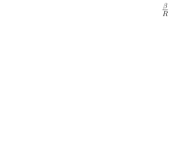
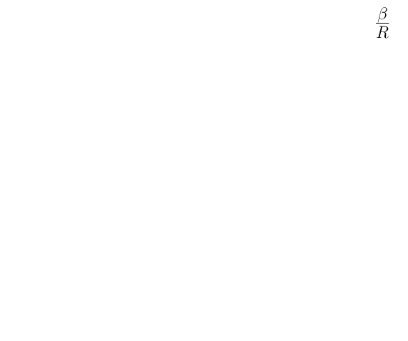
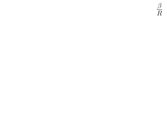
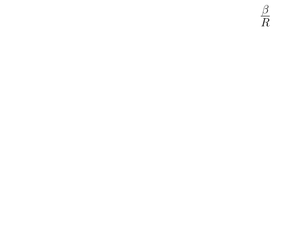
L≡(β−2​π​R)​∂∂β​log⁡Z−log⁡Z≥0,\begin{split}L\equiv(\beta-2\pi R)\frac{\partial}{\partial\beta}\log Z-\log Z\geq 0\,,\end{split} (6)

which shows that LL is an additive quantity, at zero ’t Hooft coupling, such that if L≥0L\geq 0 is true separately for scalars, fermions, and vectors, then it is true for all theories which contain a combination of these fields.

Following [8] we will test the validity of the Bekenstein bound by obtaining the minimum of LL when possible. The derivatives of LL with respect to β\beta,

∂L∂β=(β−2​π​R)​∂2∂β2​log⁡Z,∂2L∂β2=∂2∂β2​log⁡Z+(β−2​π​R)​∂3∂β3​log⁡Z,\begin{split}\frac{\partial L}{\partial\beta}&=(\beta-2\pi R)\frac{\partial^{2}}{\partial\beta^{2}}\log Z\,,\\ \frac{\partial^{2}L}{\partial\beta^{2}}&=\frac{\partial^{2}}{\partial\beta^{2}}\log Z+(\beta-2\pi R)\frac{\partial^{3}}{\partial\beta^{3}}\log Z\,,\end{split} (7)

indicate that LL has a minimum at β=2​π​R\beta=2\pi R when ∂2∂β2​log⁡Z>0\frac{\partial^{2}}{\partial\beta^{2}}\log Z>0. In this case satisfaction of the Bekenstein bound implies that

−log⁡Z|β=2​π​R≥0,\begin{split}-\log Z\Big|_{\beta=2\pi R}\geq 0\,,\end{split} (8)

or equivalently that

F|β=2​π​R≥0.\begin{split}F\Big|_{\beta=2\pi R}\geq 0\,.\end{split} (9)

Following [9, 2, 8] we derive the high temperature partition functions for theories with massless scalars, vectors, and fermions, then consider theories with massive fermions and scalars. The calculations are carried out for d=3d=3 spatial dimensions but they proceed in a similar manner for any dd. In each case we evaluate LL using (6) to determine if the Bekenstein bound is satisfied. It turns out that this depends on whether the Casimir (zero-point) energy contribution is included in log⁡Z\log Z, and, in the case of massive matter, on how it is regularized.

2 Partition functions

Although it is possible to obtain the partition functions at zero ’t Hooft coupling from counting arguments we summarize how they are calculated from one-loop perturbation theory, following [10], as a physical motivation, and as a basis for considering interacting theories. The one-loop results are valid at all temperatures when the radius of the S3S^{3} is much less than the inverse strong coupling scale, R<<ΛY​M−1R<<\Lambda_{YM}^{-1}. The contribution to the partition function from NsN_{s} real scalars with mass mm is 22 2 Here we use the saddle point approximation to relate the action to the partition function via S=−log⁡ZS=-\log Z such that the integrals over AμA_{\mu} evaluate to the stationary point solution. This is valid, for example, for S​U​(Nc)SU(N_{c}) or U⁡(Nc)U(N_{c}) theories at large NcN_{c}.

log⁡Zs=−Ns2​log⁡det⁡[−D02−Δ(s)+m2],\begin{split}\log Z_{s}=-\frac{N_{s}}{2}\log{\rm det}\left[-D_{0}^{2}-\Delta^{(s)}+m^{2}\right]\,,\end{split} (10)

where Δ(s)\Delta^{(s)} is the (conformally coupled) scalar Laplacian. Its eigenvalues εl(s)\varepsilon^{(s)}_{l} and degeneracies dl(s)d_{l}^{(s)} on S3S^{3} with radius RR take the form

Δ(s)​Yl​(Ω^)=−εl(s)​2​Yl​(Ω^),εl(s)=1R​(l+1),dl(s)=(l+1)2,\begin{split}\Delta^{(s)}Y_{l}({\hat{\Omega}})&=-\varepsilon_{l}^{(s)2}Y_{l}({\hat{\Omega}})\,,\\ \varepsilon_{l}^{(s)}&=\tfrac{1}{R}(l+1)\,,\\ d_{l}^{(s)}&=(l+1)^{2}\,,\end{split} (11)

where l=0,1,2,…l=0,1,2,....

For vector theories, the spatial gauge field can be decomposed as Ai=Bi+CiA_{i}=B_{i}+C_{i} where BiB_{i} give the transverse components with ∇iBi=0\nabla_{i}B_{i}=0, and CiC_{i} give the longitudinal components with Ci=∇ifC_{i}=\nabla_{i}f. The temporal gauge field is decomposed as A0=α+g​𝒜0A_{0}=\alpha+g{\cal A}_{0}, where the background field α\alpha contains the diagonal elements of A0A_{0} and g​𝒜0g{\cal A}_{0} contains the off-diagonal elements. Then, keeping the one-loop contributions, the CiC_{i} cancel almost completely against the ghost contribution and the off-diagonal fluctuations of the temporal gauge field. What remains is the Vandermonde contribution

log⁡ZV​d​m=12​log⁡detl=0​(−D02−Δ(s,min)),\begin{split}\log Z_{Vdm}=\frac{1}{2}\log{\rm det}_{l=0}\left(-D_{0}^{2}-\Delta^{(s,{\rm min})}\right)\,,\end{split} (12)

which is the Jacobian factor necessary for converting between a unitary matrix and its eigenvalue angles. The relevant energy eigenvalues εl(s,min)\varepsilon^{(s,{\rm min})}_{l} and degeneracies dl(s)d_{l}^{(s)} of the (minimally coupled) scalar Laplacian Δ(s,min)\Delta^{(s,{\rm min})} on S3S^{3} are

Δ(s,min)​Yl​(Ω^)=−εl(s,min)​2​Yl​(Ω^),εl(s,min)​2=1R​l​(l+2),dl(s)=(l+1)2,\begin{split}\Delta^{(s,{\rm min})}Y_{l}({\hat{\Omega}})&=-\varepsilon_{l}^{(s,{\rm min})2}Y_{l}({\hat{\Omega}})\,,\\ \varepsilon_{l}^{(s,{\rm min})2}&=\tfrac{1}{R}l(l+2)\,,\\ d_{l}^{(s)}&=(l+1)^{2}\,,\end{split} (13)

where l=0,1,2,…l=0,1,2,....

The contribution of the remaining (transverse) vectors BiB^{i}, to the partition function is

log⁡Zv=−12​log⁡det⁡[−D02−Δ(v)].\begin{split}\log Z_{v}=-\frac{1}{2}\log{\rm det}\left[-D_{0}^{2}-\Delta^{(v)}\right]\,.\end{split} (14)

The eigenvalues εl(v)\varepsilon^{(v)}_{l} and degeneracies dl(v)d_{l}^{(v)} of the transverse vector Laplacian Δ(v)\Delta^{(v)} on S3S^{3} are

Δ(v)​Bli​(Ω^)=−εl(v)​2​Bli​(Ω^),εl(v)=1R​(l+1),dl(v)=2​l​(l+2),\begin{split}\Delta^{(v)}B^{i}_{l}({\hat{\Omega}})&=-\varepsilon_{l}^{(v)2}B^{i}_{l}({\hat{\Omega}})\,,\\ \varepsilon_{l}^{(v)}&=\tfrac{1}{R}(l+1)\,,\\ d_{l}^{(v)}&=2l(l+2)\,,\end{split} (15)

where l=1,2,…l=1,2,....

The contribution of NfN_{f} (Majorana) fermions of mass mm is

log⁡Zf=Nf​log⁡det⁡[−D02−Δ(f)+14​ℛ+m2],\begin{split}\log Z_{f}=N_{f}\log{\rm det}\left[-D_{0}^{2}-\Delta^{(f)}+\frac{1}{4}{\mathscr{R}}+m^{2}\right]\,,\end{split} (16)

where ℛ{\mathscr{R}} is the scalar curvature of S3S^{3}. The eigenvalues εl(f)\varepsilon^{(f)}_{l} and degeneracies dl(f)d_{l}^{(f)} of the fermion Laplacian Δ(f)\Delta^{(f)} on S3S^{3} are

(Δ(f)−14​ℛ)​ψ=−εl(f)​2​ψ,εl(f)=1R​(l+12),dl(f)=l⁡(l+1),\begin{split}\left(\Delta^{(f)}-\frac{1}{4}{\mathscr{R}}\right)\psi&=-\varepsilon_{l}^{(f)2}\psi\,,\\ \varepsilon_{l}^{(f)}&=\tfrac{1}{R}(l+\tfrac{1}{2})\,,\\ d_{l}^{(f)}&=l(l+1)\,,\end{split} (17)

where l=1,2,…l=1,2,....

In terms of the constant background temporal gauge field, Aμ=δμ​0​αA_{\mu}=\delta_{\mu 0}\alpha, the partition functions for fields in the representation ℛ{\cal R} can be calculated by using the decomposition D0=∂0+iα→iωn±+iαD_{0}=\partial_{0}+i\alpha\rightarrow i\omega_{n}^{\pm}+i\alpha, then taking the determinants over momentum space to obtain

det​(−D02+ε2)±=det(−(∂0+iα)2+ε2),=detℛ​∏l∏n∈ℤ((ωn±+α)2+εl2+m2)dl,\begin{split}{\rm det}(-D_{0}^{2}+\varepsilon^{2})_{\pm}&={\rm det}\left(-(\partial_{0}+i\alpha)^{2}+\varepsilon^{2}\right)\,,\\ &={\rm det}_{{\cal R}}\prod_{l}\prod_{n\in{\mathbb{Z}}}\left((\omega_{n}^{\pm}+\alpha)^{2}+\varepsilon_{l}^{2}+m^{2}\right)^{d_{l}}\,,\end{split} (18)

where the Matsubara frequencies are ωn+=2​π​nβ\omega_{n}^{+}=\frac{2\pi n}{\beta} for fields with periodic boundary conditions around S1S^{1}, and ωn−=(2​n+1)​πβ\omega_{n}^{-}=\frac{(2n+1)\pi}{\beta} for fields with antiperiodic boundary conditions. Following [10] for fields with periodic boundary conditions

∏n∈ℤ((ωn++α)2+ε2)=(α2+ε2)​∏k≠0[4​π2​k2β2]​∏n=1∞[(1−β2​(α+i​ε)24​π2​n2)​(1−β2​(α−i​ε)24​π2​n2)],=4β2​∏k=1∞[16​π4​k4β4]​sin⁡[β2​(α+i​ε)]​sin⁡[β2​(α−i​ε)],=𝒩​eβ​ε​(1−e−β​ε+i​β​α)​(1−e−β​ε−i​β​α),\begin{split}&\prod_{n\in{\mathbb{Z}}}\left((\omega_{n}^{+}+\alpha)^{2}+\varepsilon^{2}\right)\\ &=(\alpha^{2}+\varepsilon^{2})\prod_{k\neq 0}\left[\frac{4\pi^{2}k^{2}}{\beta^{2}}\right]\prod_{n=1}^{\infty}\left[\left(1-\frac{\beta^{2}(\alpha+i\varepsilon)^{2}}{4\pi^{2}n^{2}}\right)\left(1-\frac{\beta^{2}(\alpha-i\varepsilon)^{2}}{4\pi^{2}n^{2}}\right)\right]\,,\\ &=\frac{4}{\beta^{2}}\prod_{k=1}^{\infty}\left[\frac{16\pi^{4}k^{4}}{\beta^{4}}\right]\sin\left[\frac{\beta}{2}(\alpha+i\varepsilon)\right]\sin\left[\frac{\beta}{2}(\alpha-i\varepsilon)\right]\,,\\ &={\cal N}e^{\beta\varepsilon}\left(1-e^{-\beta\varepsilon+i\beta\alpha}\right)\left(1-e^{-\beta\varepsilon-i\beta\alpha}\right)\,,\end{split} (19)

where the identity ∏n=1∞(1−x2n2)=sin⁡(π​x)π​x\prod_{n=1}^{\infty}\left(1-\frac{x^{2}}{n^{2}}\right)=\frac{\sin(\pi x)}{\pi x} was used to obtain the third line, and

𝒩≡1β2​∏k=1∞[16​π4​k4β4].\begin{split}{\cal N}\equiv\frac{1}{\beta^{2}}\prod_{k=1}^{\infty}\left[\frac{16\pi^{4}k^{4}}{\beta^{4}}\right]\,.\end{split} (20)

Following the same procedure for fields with antiperiodic boundary conditions around S1S^{1} results in the replacement α→α+πβ\alpha\rightarrow\alpha+\frac{\pi}{\beta}. That is,

∏n∈ℤ((ωn−+α)2+ε2)=𝒩​eβ​ε​(1+e−β​ε+i​β​α)​(1+e−β​ε−i​β​α).\begin{split}\prod_{n\in{\mathbb{Z}}}\left((\omega_{n}^{-}+\alpha)^{2}+\varepsilon^{2}\right)={\cal N}e^{\beta\varepsilon}\left(1+e^{-\beta\varepsilon+i\beta\alpha}\right)\left(1+e^{-\beta\varepsilon-i\beta\alpha}\right)\,.\end{split} (21)

Putting it all together, shifting α\alpha to the new independent variable θ≡β​α\theta\equiv\beta\alpha such that θ=diag⁡{θ1,θ2,…,θNc}\theta={\rm diag}\{\theta_{1},\theta_{2},...,\theta_{N_{c}}\} is the matrix of eigenvalue angles of the Polyakov lines 𝒫n(ℛ)≡Trℛ​ei​n​β​α=Trℛ​ei​n​θ{\mathscr{P}}_{n}^{({\cal R})}\equiv{\rm Tr}_{{\cal R}}e^{in\beta\alpha}={\rm Tr}_{{\cal R}}e^{in\theta}, gives the result

log⁡det​(−D02+ε2)±=dℛ​β​∑ldl​εl−∑n=1∞(±1)nn​∑ldl​e−n​β​εl​[Trℛ​ei​n​θ+Trℛ​e−i​n​θ],\begin{split}\log{\rm det}(-D_{0}^{2}+\varepsilon^{2})_{\pm}=d_{{\cal R}}\beta\sum_{l}d_{l}\varepsilon_{l}-\sum_{n=1}^{\infty}\frac{(\pm 1)^{n}}{n}\sum_{l}d_{l}e^{-n\beta\varepsilon_{l}}\left[{\rm Tr}_{{\cal R}}e^{in\theta}+{\rm Tr}_{{\cal R}}e^{-in\theta}\right]\,,\end{split} (22)

for fields in the representation ℛ{\cal R}, with dimension dℛd_{{\cal R}}. The top sign in (22) is for fields with periodic boundary conditions around S1S^{1} and the bottom sign is for fields with antiperiodic boundary conditions. The absence of an 𝒩{\cal N}-dependent term in (22) results from

log⁡𝒩=−2​log⁡β+4​∑k=1∞[log⁡(2​πβ)+log⁡k],=−2​log⁡β+4​log⁡(2​πβ)​ζ​(0)−4​ζ′​(0),=0.\begin{split}\log{\cal N}&=-2\log\beta+4\sum_{k=1}^{\infty}\left[\log\left(\frac{2\pi}{\beta}\right)+\log k\right]\,,\\ &=-2\log\beta+4\log\left(\frac{2\pi}{\beta}\right)\zeta(0)-4\zeta^{\prime}(0)\,,\\ &=0\,.\end{split} (23)

Using (22) the Vandermonde contribution becomes

log⁡ZV​d​m=12​d𝒜​β​d0​ε0−∑n=1∞1n​d0​e−n​β​ε0​Tr𝒜​ei​n​θ,=−∑n=1∞1nTr𝒜ei​n​θ,\begin{split}\log Z_{Vdm}&=\frac{1}{2}d_{{\cal A}}\beta d_{0}\varepsilon_{0}-\sum_{n=1}^{\infty}\frac{1}{n}d_{0}e^{-n\beta\varepsilon_{0}}{\rm Tr}_{{\cal A}}e^{in\theta}\,,\\ &=-\sum_{n=1}^{\infty}\frac{1}{n}{\rm Tr}_{{\cal A}}e^{in\theta}\,,\end{split} (24)

where d𝒜d_{{\cal A}} is the dimension of the adjoint representation. In the calculations of the high temperature partition functions that follow we drop this contribution. From (24) one finds that in the high temperature deconfined phase Tr𝒜​ei​n​θ→d𝒜{\rm Tr}_{{\cal A}}e^{in\theta}\rightarrow d_{{\cal A}} and log⁡ZV​d​m→−d𝒜​ζ​(1)\log Z_{Vdm}\rightarrow-d_{{\cal A}}\zeta(1). In the low temperature confined phase, Tr𝒜​ei​n​θ→0{\rm Tr}_{{\cal A}}e^{in\theta}\rightarrow 0 for U⁡(Nc)U(N_{c}) vectors, and Tr𝒜​ei​n​θ→−1{\rm Tr}_{{\cal A}}e^{in\theta}\rightarrow-1 for S​U​(Nc)SU(N_{c}) vectors such that log⁡ZV​d​m→0\log Z_{Vdm}\rightarrow 0 or ζ⁡(1)\zeta(1), respectively. For the S​U​(Nc)SU(N_{c}) theory it is necessary to shift the temperature behavior of log⁡ZV​d​m\log Z_{Vdm} from ζ⁡(1)\zeta(1) to zero such that the entropy S→0S\rightarrow 0 at zero temperature, following [1], to satisfy the third law of thermodynamics. The high temperature contribution should be considered more carefully. In order that the free energy doesn’t slowly diverge we impose the requirement that limn→∞Tr𝒜​ei​n​θ=0\lim_{n\rightarrow\infty}{\rm Tr}_{{\cal A}}e^{in\theta}=0. This allows the sum to be truncated. In the high temperature limit the result is logZV​d​m≃−d𝒜∑n=1Λ1n≃−d𝒜(logΛ+γE)\log Z_{Vdm}\simeq-d_{{\cal A}}\sum_{n=1}^{\Lambda}\frac{1}{n}\simeq-d_{{\cal A}}(\log\Lambda+\gamma_{E}), where Λ\Lambda is large. This truncated result can be dominated by contributions from the single particle partition functions for the matter fields in the high temperature limit, allowing for the recovery of the expected one-loop free energy and other thermodynamic observables as R→∞R\rightarrow\infty. Using (6) the Vandermonde term contributes favorably towards satisfaction of the Bekenstein bound with LV​d​m=−log⁡ZV​d​m≃d𝒜​(log⁡Λ+γE)L_{Vdm}=-\log Z_{Vdm}\simeq d_{{\cal A}}(\log\Lambda+\gamma_{E}). In what follows we will ignore this contribution since Λ\Lambda has an unknown temperature dependence, but we keep in mind that it can only help the Bekenstein bound to be satisfied. Dropping this term entirely is valid deep in the deconfined phase in the very high temperature limit (The Vandermonde term can be included in the calculation of the vector partition function as in [10]. The partition function can then be precisely calculated at very high temperatures but numerical checks are not possible.). If we wished to study the theory close to a deconfinement-confinement transition then consideration of the θ\theta-dependence of the Vandermonde piece would be crucial.

3 Casimir Energy

The Casimir energies for real scalars and Weyl fermions in the representation ℛ{\cal R}, and adjoint vectors, are given by, respectively,

EC​a​s(s)=dℛ(s)2​R​∑ldl(s)​εl(s),EC​a​s(f)=−dℛ(f)R∑ldl(f)εl(f),EC​a​s(v)=d𝒜2​R​∑ldl(v)​εl(v).\begin{split}E_{Cas}^{(s)}&=\frac{d_{{\cal R}}^{(s)}}{2R}\sum_{l}d_{l}^{(s)}\varepsilon_{l}^{(s)}\,,\\ E_{Cas}^{(f)}&=-\frac{d_{{\cal R}}^{(f)}}{R}\sum_{l}d_{l}^{(f)}\varepsilon_{l}^{(f)}\,,\\ E_{Cas}^{(v)}&=\frac{d_{{\cal A}}}{2R}\sum_{l}d_{l}^{(v)}\varepsilon_{l}^{(v)}\,.\end{split} (25)

To obtain the Casimir energies it is necessary to regulate the sums. When the matter is massless it is straightforward to perform these sums using zeta function regularization. When it is massive, it is unclear how to obtain the appropriately regularized result. One option is to obtain results using a cutoff regularization scheme and compare with those using zeta function regularization to define an undetermined regularization parameter and obtain a, perhaps scheme independent, result. Another possibility is to use only zeta function regularization then apply a physical constraint to obtain the undetermined regularization parameter, namely, considering the masses as quantum corrections such that their contribution to the energy is constrained to vanish as the mass is taken to infinity.

3.1 Scalars

For real scalars with mass mm the Casimir energy is

EC​a​s(s)=dℛ(s)2​R​∑l=0∞(l+1)2​(l+1)2+m2​R2.\begin{split}E_{Cas}^{(s)}&=\frac{d_{{\cal R}}^{(s)}}{2R}\sum_{l=0}^{\infty}(l+1)^{2}\sqrt{(l+1)^{2}+m^{2}R^{2}}\,.\end{split} (26)

In the massless limit it is straightforward to obtain the Casimir energy using zeta function regularization,

EC​a​s(s)|m​R=0=dℛ(s)2​R​∑l=1∞l3=dℛ(s)2​R​ζ​(−3)=dℛ(s)240​R.\begin{split}E_{Cas}^{(s)}\Big|_{mR=0}&=\frac{d_{{\cal R}}^{(s)}}{2R}\sum_{l=1}^{\infty}l^{3}=\frac{d_{{\cal R}}^{(s)}}{2R}\zeta(-3)=\frac{d_{{\cal R}}^{(s)}}{240R}\,.\end{split} (27)

When m​R≠0mR\neq 0 it is more complicated to regularize the sum. First we follow [11] and consider two regularization schemes: cutoff regularization, and zeta function regularization. We match the zeta function regularized result against the cutoff-independent part of the cutoff-regularized result to obtain the appropriate normalization. Second, we calculate the Casimir energy using the constraint that it vanishes as the mass goes to infinity reproducing the results in [7, 12]. In both cases the zeta function regularization procedure in [13] is used.

3.1.1 Cutoff regularization

Following [11] we define the cutoff regularized Casimir energy for a real scalar field as

EC​a​s(s)(λ)≡−dℛ(s)2​R∂∂λ∑l=0∞(l+1)2e−λ​(l+1)2+m2​R2.\begin{split}E_{Cas}^{(s)}(\lambda)\equiv-\frac{d_{{\cal R}}^{(s)}}{2R}\frac{\partial}{\partial\lambda}\sum_{l=0}^{\infty}(l+1)^{2}e^{-\lambda\sqrt{(l+1)^{2}+m^{2}R^{2}}}\,.\end{split} (28)

To solve the sum it is useful to express the exponential as a contour integral via the Mellin Transform

e−x=12​π​i​∫𝒞d​s​Γ​(s)​x−s,\begin{split}e^{-x}=\frac{1}{2\pi i}\int_{{\cal C}}{\rm d}s\,\Gamma(s)x^{-s}\,,\end{split} (29)

where the contour 𝒞{\cal C} extends from c0−i​∞c_{0}-i\infty to c0+i​∞c_{0}+i\infty with c0>3c_{0}>3 (for dd dimensions c0>d−1c_{0}>d-1) to allow the sum over ll to be brought into the integral. The Casimir energy is then

EC​a​s(s)(λ)=−dℛ(s)2​R∂∂λ12​π​i∫𝒞dsGs(s),\begin{split}E_{Cas}^{(s)}(\lambda)=-\frac{d_{{\cal R}}^{(s)}}{2R}\frac{\partial}{\partial\lambda}\frac{1}{2\pi i}\int_{{\cal C}}{\rm d}s\,G_{s}(s)\,,\end{split} (30)

with

Gs​(s)=λ−sΓ(s)∑l=0∞(l+1)2[(l+1)2+m2R2]−s/2=λ−sΓ(s)∑l=1∞[[l2+m2R2]1−s/2−m2R2[l2+m2R2]−s/2].\begin{split}G_{s}(s)&=\lambda^{-s}\Gamma(s)\sum_{l=0}^{\infty}(l+1)^{2}[(l+1)^{2}+m^{2}R^{2}]^{-s/2}\\ &=\lambda^{-s}\Gamma(s)\sum_{l=1}^{\infty}\bigg[\left[l^{2}+m^{2}R^{2}\right]^{1-s/2}-m^{2}R^{2}\left[l^{2}+m^{2}R^{2}\right]^{-s/2}\bigg]\,.\end{split} (31)

The sum over ll can be solved by zeta function regularization using (1.38) in [14] (see also [7, 12]),

∑l=1∞(l2+M2)−s=−M−2​s2+π2​M−2​s+1​Γ⁡(s−12)Γ⁡(s)+2​πsΓ⁡(s)M−s+1/2∑n=1∞ns−1/2Ks−1/2(2πnM).\begin{split}\sum_{l=1}^{\infty}\left(l^{2}+M^{2}\right)^{-s}=&-\frac{M^{-2s}}{2}+\frac{\sqrt{\pi}}{2}M^{-2s+1}\frac{\Gamma(s-\frac{1}{2})}{\Gamma(s)}\\ &+\frac{2\pi^{s}}{\Gamma(s)}M^{-s+1/2}\sum_{n=1}^{\infty}n^{s-1/2}K_{s-1/2}(2\pi nM)\,.\end{split} (32)

Note that the sum converges to this result for s>12s>\frac{1}{2} and this is why the contour was required to have c0>3c_{0}>3. (32) also gives the appropriate analytic continuation for other ss. Using this result gives

Gs​(s)=λ−s2sΓ(s+12)[18(mR)3−sΓ(s−32)+∑n=1∞[(s2−1)(π​nm​R)(s−3)/2Ks−32(2πnmR)−m2R2(π​nm​R)(s−1)/2Ks−12(2πnmR)]].\begin{split}G_{s}(s)=&\lambda^{-s}2^{s}\Gamma(\tfrac{s+1}{2})\bigg[\frac{1}{8}(mR)^{3-s}\Gamma(\tfrac{s-3}{2})+\sum_{n=1}^{\infty}\bigg[(\tfrac{s}{2}-1)\left(\frac{\pi n}{mR}\right)^{(s-3)/2}K_{\frac{s-3}{2}}(2\pi nmR)\\ &\hskip 68.2866pt-m^{2}R^{2}\left(\frac{\pi n}{mR}\right)^{(s-1)/2}K_{\frac{s-1}{2}}(2\pi nmR)\bigg]\bigg]\,.\end{split} (33)

The next step is to add an arc at infinity in the left-hand complex ss-plane to close the contour in (30) around the poles in Gs​(s)G_{s}(s) and collect the residues. The contribution of this arc alone to the contour integral is negligible for sufficiently small values of λ\lambda. Evaluating Gs​(s)G_{s}(s) at the ss-values corresponding to singularities in the Gamma functions gives rise to the relevant simple poles

Gs​(s→3)∝(1s−3)​2λ3,Gs​(s→1)∝−(1s−1)​m2​R22​λ,Gs(s→−1)∝(1s+1)λ{m4R4[332−18γE+18log(2λ​m​R)]−∑n=1∞[32(m​Rπ​n)2K2(2πnmR)+m2R2(m​Rπ​n)K1(2πnmR)]}.\begin{split}&G_{s}(s\rightarrow 3)\propto\left(\frac{1}{s-3}\right)\frac{2}{\lambda^{3}}\,,\\ &G_{s}(s\rightarrow 1)\propto-\left(\frac{1}{s-1}\right)\frac{m^{2}R^{2}}{2\lambda}\,,\\ &G_{s}(s\rightarrow-1)\propto\left(\frac{1}{s+1}\right)\lambda\,\Bigg\{m^{4}R^{4}\bigg[\frac{3}{32}-\frac{1}{8}\gamma_{E}+\frac{1}{8}\log\left(\frac{2}{\lambda mR}\right)\bigg]\\ &\hskip 68.2866pt-\sum_{n=1}^{\infty}\left[\frac{3}{2}\left(\frac{mR}{\pi n}\right)^{2}K_{2}(2\pi nmR)+m^{2}R^{2}\left(\frac{mR}{\pi n}\right)K_{1}(2\pi nmR)\right]\Bigg\}\,.\end{split} (34)

The remaining simple poles (for s=−3,−5,…s=-3,-5,...) are higher order in λ\lambda and produce negligible, cutoff-dependent contributions, even after taking the λ\lambda-derivative in (28). Collecting the residues the cutoff-regularized Casimir energy takes the final form

EC​a​s(s)​(λ)≃dℛ(s)2​R{6λ4−m2​R22​λ2+m4R4[132+18γE+18log(λ​m​R2)]+∑n=1∞[32(m​Rπ​n)2K2(2πnmR)+m2R2(m​Rπ​n)K1(2πnmR)]}.\begin{split}E_{Cas}^{(s)}(\lambda)\simeq&\frac{d_{{\cal R}}^{(s)}}{2R}\Bigg\{\frac{6}{\lambda^{4}}-\frac{m^{2}R^{2}}{2\lambda^{2}}+m^{4}R^{4}\bigg[\frac{1}{32}+\frac{1}{8}\gamma_{E}+\frac{1}{8}\log\left(\frac{\lambda mR}{2}\right)\bigg]\\ &+\sum_{n=1}^{\infty}\left[\frac{3}{2}\left(\frac{mR}{\pi n}\right)^{2}K_{2}(2\pi nmR)+m^{2}R^{2}\left(\frac{mR}{\pi n}\right)K_{1}(2\pi nmR)\right]\Bigg\}\,.\end{split} (35)

3.1.2 Zeta function regularization

To obtain the zeta function regularized Casimir energy we follow the scheme in [13]. The Casimir energy is defined as

EC​a​s(s)​(μ)=dℛ(s)2​R​12​limε→0[ζp​(−12+ε)+ζp​(−12−ε)],\begin{split}E_{Cas}^{(s)}(\mu)=\frac{d_{{\cal R}}^{(s)}}{2R}\frac{1}{2}\lim_{\varepsilon\rightarrow 0}\left[\zeta_{p}(-\tfrac{1}{2}+\varepsilon)+\zeta_{p}(-\tfrac{1}{2}-\varepsilon)\right]\,,\end{split} (36)

where

ζp​(s)≡μ1+2​s​∑l=0∞(l+1)2​[(l+1)2+m2​R2]−s,\begin{split}\zeta_{p}(s)\equiv\mu^{1+2s}\sum_{l=0}^{\infty}(l+1)^{2}\left[(l+1)^{2}+m^{2}R^{2}\right]^{-s}\,,\end{split} (37)

and μ\mu is a normalization factor to be determined later. Dividing the sum into parts which can be separately regularized using zeta function techniques gives

ζp​(s)=μ1+2​s​∑l=1∞[[l2+m2​R2]1−s−m2​R2​[l2+m2​R2]−s].\begin{split}\zeta_{p}(s)=\mu^{1+2s}\sum_{l=1}^{\infty}\bigg[\left[l^{2}+m^{2}R^{2}\right]^{1-s}-m^{2}R^{2}\left[l^{2}+m^{2}R^{2}\right]^{-s}\bigg]\,.\end{split} (38)

Then, using (32), the Casimir energy takes the μ\mu-dependent form

EC​a​s(s)​(μ)=dℛ(s)2​R{m4R4[132+18log(m​R2​μ)]+∑n=1∞[32(m​Rπ​n)2K2(2πnmR)+m2R2(m​Rπ​n)K1(2πnmR)]}.\begin{split}E_{Cas}^{(s)}(\mu)=&\frac{d_{{\cal R}}^{(s)}}{2R}\Bigg\{m^{4}R^{4}\left[\frac{1}{32}+\frac{1}{8}\log\left(\frac{mR}{2\mu}\right)\right]\\ &+\sum_{n=1}^{\infty}\left[\frac{3}{2}\left(\frac{mR}{\pi n}\right)^{2}K_{2}(2\pi nmR)+m^{2}R^{2}\left(\frac{mR}{\pi n}\right)K_{1}(2\pi nmR)\right]\Bigg\}\,.\end{split} (39)

Comparing this result with the cutoff-independent contributions in (35) we obtain the value of the finite normalization factor, μ≡e−γE\mu\equiv e^{-\gamma_{E}}, as found in the system in [11]. We refer to the μ≡e−γE\mu\equiv e^{-\gamma_{E}}-regularized Casimir energy as the scheme II result, given by

EC​a​s(s)​I=dℛ(s)2​R{m4R4[132+18γE+18log(m​R2)]+∑n=1∞[32(m​Rπ​n)2K2(2πnmR)+m2R2(m​Rπ​n)K1(2πnmR)]}.\begin{split}E_{Cas}^{(s)I}=&\frac{d_{{\cal R}}^{(s)}}{2R}\Bigg\{m^{4}R^{4}\left[\frac{1}{32}+\frac{1}{8}\gamma_{E}+\frac{1}{8}\log\left(\frac{mR}{2}\right)\right]\\ &+\sum_{n=1}^{\infty}\left[\frac{3}{2}\left(\frac{mR}{\pi n}\right)^{2}K_{2}(2\pi nmR)+m^{2}R^{2}\left(\frac{mR}{\pi n}\right)K_{1}(2\pi nmR)\right]\Bigg\}\,.\end{split} (40)

Another way to regularize the Casimir energy is to impose the physically-motivated constraint that the matter contribution should vanish in the large mass limit [15]. The terms which diverge as m​R→∞mR\rightarrow\infty can be removed by an appropriate definition of μ\mu. In this case μ≡12​e1/4​m​R\mu\equiv\frac{1}{2}e^{1/4}mR, and the resulting Casimir energy is referred to as the scheme I​III result, given by

EC​a​s(s)​I​I=dℛ(s)2​R​∑n=1∞[32​(m​Rπ​n)2​K2​(2​π​n​m​R)+m2​R2​(m​Rπ​n)​K1​(2​π​n​m​R)],\begin{split}E_{Cas}^{(s)II}=&\frac{d_{{\cal R}}^{(s)}}{2R}\sum_{n=1}^{\infty}\left[\frac{3}{2}\left(\frac{mR}{\pi n}\right)^{2}K_{2}(2\pi nmR)+m^{2}R^{2}\left(\frac{mR}{\pi n}\right)K_{1}(2\pi nmR)\right]\,,\end{split} (41)

in agreement with [7, 12].

A few comments are in order with regard to choosing a regularization scheme. It is clear that a scalar theory regularized according to scheme II results in EC​a​s<0E_{Cas}<0 for a range of m​RmR. As discussed in [1] this leads to a partition function that can violate the entropy bound (1). This is clear by considering the large βR\frac{\beta}{R} limit where the only remaining contribution to the partition function is that of the Casimir energy. Then L=−2​π​Rβ​log⁡Z=2​π​R​EC​a​sL=-\frac{2\pi R}{\beta}\log Z=2\pi RE_{Cas}, which violates the Bekenstein bound when EC​a​s<0E_{Cas}<0. However, if scheme I​III is chosen then EC​a​s>0E_{Cas}>0 for all m​RmR and the Bekenstein bound is satisfied in this limit.

3.2 Fermions

For Weyl (Majorana) fermions with mass mm the Casimir energy is

EC​a​s(f)=−dℛ(f)R∑l=0∞l(l+1)(l+12)2+m2​R2.\begin{split}E_{Cas}^{(f)}=-\frac{d_{{\cal R}}^{(f)}}{R}\sum_{l=0}^{\infty}l(l+1)\sqrt{(l+\tfrac{1}{2})^{2}+m^{2}R^{2}}\,.\end{split} (42)

In the massless limit the Casimir energy is obtained by ordinary zeta function regularization, such that

EC​a​s(f)|m​R=0=−dℛ(f)R∑l=0∞l(l+1)(l+12)=−dℛ(f)R[ζ(−3,12)−14ζ(−1,12)]=17​dℛ(f)960​R.\begin{split}E_{Cas}^{(f)}\Big|_{mR=0}=-\frac{d_{{\cal R}}^{(f)}}{R}\sum_{l=0}^{\infty}l(l+1)(l+\tfrac{1}{2})=-\frac{d_{{\cal R}}^{(f)}}{R}\left[\zeta(-3,\tfrac{1}{2})-\frac{1}{4}\zeta(-1,\tfrac{1}{2})\right]=\frac{17d_{{\cal R}}^{(f)}}{960R}\,.\end{split} (43)

For m​R≠0mR\neq 0 we proceed as for scalars and first obtain a regularized Casimir energy by comparing results from cutoff regularization and zeta function regularization, and second by using only zeta function regularization and imposing the constraint
limm​R→∞EC​a​s=0\lim_{mR\rightarrow\infty}E_{Cas}=0.

3.2.1 Cutoff regularization

Following the procedure for scalars the cutoff regularized Casimir energy for fermions is

EC​a​s(f)​(λ)≡dℛ(f)R​∂∂λ​∑l=0∞l⁡(l+1)​e−λ​(l+12)2+m2​R2,=dℛ(f)R​∂∂λ​12​π​i​∫𝒞d​s​Gf​(s),\begin{split}E_{Cas}^{(f)}(\lambda)&\equiv\frac{d_{{\cal R}}^{(f)}}{R}\frac{\partial}{\partial\lambda}\sum_{l=0}^{\infty}l(l+1)e^{-\lambda\sqrt{(l+\frac{1}{2})^{2}+m^{2}R^{2}}}\,,\\ &=\frac{d_{{\cal R}}^{(f)}}{R}\frac{\partial}{\partial\lambda}\frac{1}{2\pi i}\int_{{\cal C}}{\rm d}s\,G_{f}(s)\,,\end{split} (44)

with

Gf​(s)=λ−sΓ(s)∑l=0∞l(l+1)[(l+12)2+m2R2]−s/2,=λ−sΓ(s)∑l=0∞[[(l+12)2+m2R2]1−s/2−(14+m2R2)[(l+12)2+m2R2]−s/2].\begin{split}G_{f}(s)&=\lambda^{-s}\Gamma(s)\sum_{l=0}^{\infty}l(l+1)[(l+\tfrac{1}{2})^{2}+m^{2}R^{2}]^{-s/2}\,,\\ &=\lambda^{-s}\Gamma(s)\sum_{l=0}^{\infty}\bigg[\left[(l+\tfrac{1}{2})^{2}+m^{2}R^{2}\right]^{1-s/2}-(\tfrac{1}{4}+m^{2}R^{2})\left[(l+\tfrac{1}{2})^{2}+m^{2}R^{2}\right]^{-s/2}\bigg]\,.\end{split} (45)

The sum over ll can be solved by zeta function regularization using (4.17) in [14],

∑l=0∞[(l+12)2+M2]−s=π2​Γ⁡(s−12)Γ⁡(s)​|M|1−2​s+2​πsΓ⁡(s)|M|∑n=1∞1/2−s⁡(−1)n​ns−1/2​Ks−1/2​(2​π​n​|M|),\begin{split}&\sum_{l=0}^{\infty}\left[(l+\tfrac{1}{2})^{2}+M^{2}\right]^{-s}\\ &=\frac{\sqrt{\pi}}{2}\frac{\Gamma(s-\tfrac{1}{2})}{\Gamma(s)}|M|^{1-2s}+\frac{2\pi^{s}}{\Gamma(s)}|M|^{1/2-s}\sum_{n=1}^{\infty}(-1)^{n}n^{s-1/2}K_{s-1/2}(2\pi n|M|)\,,\end{split} (46)

where the sum converges for all s>12s>\frac{1}{2} and the result provides the appropriate analytic continuation for other ss. Using this result gives

Gf​(s)=λ−s2sΓ(s+12)[18(mR)1−s(m2R2−14(s−3))Γ(s−32)+∑n=1∞(−1)n[(s2−1)(π​nm​R)(s−3)/2Ks−32(2πnmR)−(14+m2R2)(π​nm​R)(s−1)/2Ks−12(2πnmR)]].\begin{split}G_{f}(s)=&\lambda^{-s}2^{s}\Gamma(\tfrac{s+1}{2})\bigg[\frac{1}{8}(mR)^{1-s}\left(m^{2}R^{2}-\frac{1}{4}(s-3)\right)\Gamma(\tfrac{s-3}{2})\\ &+\sum_{n=1}^{\infty}(-1)^{n}\bigg[(\tfrac{s}{2}-1)\left(\frac{\pi n}{mR}\right)^{(s-3)/2}K_{\frac{s-3}{2}}(2\pi nmR)\\ &\hskip 68.2866pt-(\tfrac{1}{4}+m^{2}R^{2})\left(\frac{\pi n}{mR}\right)^{(s-1)/2}K_{\frac{s-1}{2}}(2\pi nmR)\bigg]\bigg]\,.\end{split} (47)

Evaluating Gf​(s)G_{f}(s) at the ss-values corresponding to singularities in the Gamma functions gives rise to the relevant simple poles at s=3,1,−1s=3,1,-1. The remaining simple poles (for s=−3,−5,…s=-3,-5,...) are higher order in λ\lambda and produce negligible, cutoff-dependent contributions. Collecting the residues the cutoff-regularized Casimir energy takes the final form

EC​a​s(f)​(λ)≃dℛ(f)R{6λ4−(m2​R2+12)2​λ2+m2R2[116+132m2R2+18(1+m2R2)γE+18(1+m2R2)log(λ​m​R2)]+∑n=1∞(−1)n[32(m​Rπ​n)2K2(2πnmR)+(m2R2+14)(m​Rπ​n)K1(2πnmR)]}.\begin{split}E_{Cas}^{(f)}(\lambda)\simeq&\frac{d_{{\cal R}}^{(f)}}{R}\Bigg\{\frac{6}{\lambda^{4}}-\frac{(m^{2}R^{2}+\frac{1}{2})}{2\lambda^{2}}+m^{2}R^{2}\bigg[\frac{1}{16}+\frac{1}{32}m^{2}R^{2}+\frac{1}{8}(1+m^{2}R^{2})\gamma_{E}\\ &+\frac{1}{8}(1+m^{2}R^{2})\log\left(\frac{\lambda mR}{2}\right)\bigg]\\ &+\sum_{n=1}^{\infty}(-1)^{n}\left[\frac{3}{2}\left(\frac{mR}{\pi n}\right)^{2}K_{2}(2\pi nmR)+(m^{2}R^{2}+\tfrac{1}{4})\left(\frac{mR}{\pi n}\right)K_{1}(2\pi nmR)\right]\Bigg\}\,.\end{split} (48)

3.2.2 Zeta function regularization

To obtain the zeta function regularized Casimir energy we again follow the regularization prescription in [13], where for fermions

EC​a​s(f)(μ)=−dℛ(f)2​Rlimε→0[ζp(−12+ε)+ζp(−12−ε)],\begin{split}E_{Cas}^{(f)}(\mu)=-\frac{d_{{\cal R}}^{(f)}}{2R}\lim_{\varepsilon\rightarrow 0}\left[\zeta_{p}(-\tfrac{1}{2}+\varepsilon)+\zeta_{p}(-\tfrac{1}{2}-\varepsilon)\right]\,,\end{split} (49)

with

ζp​(s)≡μ1+2​s​∑l=0∞l⁡(l+1)​[(l+12)2+m2​R2]−s,=μ1+2​s​∑l=0∞[[(l+12)2+m2​R2]1−s−(14+m2​R2)​[(l+12)2+m2​R2]−s].\begin{split}\zeta_{p}(s)&\equiv\mu^{1+2s}\sum_{l=0}^{\infty}l(l+1)\left[(l+\tfrac{1}{2})^{2}+m^{2}R^{2}\right]^{-s}\,,\\ &=\mu^{1+2s}\sum_{l=0}^{\infty}\bigg[\left[(l+\tfrac{1}{2})^{2}+m^{2}R^{2}\right]^{1-s}-(\tfrac{1}{4}+m^{2}R^{2})\left[(l+\tfrac{1}{2})^{2}+m^{2}R^{2}\right]^{-s}\bigg]\,.\end{split} (50)

Then, using (46), the Casimir energy takes the μ\mu-dependent form

EC​a​s(f)​(μ)=−dℛ(f)R{m2R2[116+132m2R2+18(1+m2R2)log(m​R2​μ)]+∑n=1∞(−1)n[32(m​Rπ​n)2K2(2πnmR)+(m2R2+14)(m​Rπ​n)K1(2πnmR)]}.\begin{split}E_{Cas}^{(f)}(\mu)=&-\frac{d_{{\cal R}}^{(f)}}{R}\Bigg\{m^{2}R^{2}\left[\frac{1}{16}+\frac{1}{32}m^{2}R^{2}+\frac{1}{8}(1+m^{2}R^{2})\log\left(\frac{mR}{2\mu}\right)\right]\\ &+\sum_{n=1}^{\infty}(-1)^{n}\left[\frac{3}{2}\left(\frac{mR}{\pi n}\right)^{2}K_{2}(2\pi nmR)+(m^{2}R^{2}+\tfrac{1}{4})\left(\frac{mR}{\pi n}\right)K_{1}(2\pi nmR)\right]\Bigg\}\,.\end{split} (51)

Equating this result with the cutoff-independent contributions in (48) gives the normalization factor μ≡e−γE\mu\equiv e^{-\gamma_{E}}, as in the scalar case. Therefore, the μ≡e−γE\mu\equiv e^{-\gamma_{E}} scheme II-regularized fermion Casimir energy is

EC​a​s(f)​I=−dℛ(f)R{m2R2[116+132m2R2+18(1+m2R2)γE+18(1+m2R2)log(m​R2)]+∑n=1∞(−1)n[32(m​Rπ​n)2K2(2πnmR)+(m2R2+14)(m​Rπ​n)K1(2πnmR)]}.\begin{split}E_{Cas}^{(f)I}=&-\frac{d_{{\cal R}}^{(f)}}{R}\Bigg\{m^{2}R^{2}\left[\frac{1}{16}+\frac{1}{32}m^{2}R^{2}+\frac{1}{8}(1+m^{2}R^{2})\gamma_{E}+\frac{1}{8}(1+m^{2}R^{2})\log\left(\frac{mR}{2}\right)\right]\\ &+\sum_{n=1}^{\infty}(-1)^{n}\left[\frac{3}{2}\left(\frac{mR}{\pi n}\right)^{2}K_{2}(2\pi nmR)+(m^{2}R^{2}+\tfrac{1}{4})\left(\frac{mR}{\pi n}\right)K_{1}(2\pi nmR)\right]\Bigg\}\,.\end{split} (52)

For regularization scheme I​III, where the Casimir energy is required to vanish as m​R→∞mR\rightarrow\infty, the normalization factor in (51) must be chosen as μ≡12​m​R​exp⁡[2+m2​R24​(1+m2​R2)]\mu\equiv\frac{1}{2}mR\exp\left[\frac{2+m^{2}R^{2}}{4(1+m^{2}R^{2})}\right] such that the Casimir energy is reduced to

EC​a​s(f)​I​I=−dℛ(f)R∑n=1∞(−1)n[32(m​Rπ​n)2K2(2πnmR)+(m2R2+14)(m​Rπ​n)K1(2πnmR)].\begin{split}E_{Cas}^{(f)II}=&-\frac{d_{{\cal R}}^{(f)}}{R}\sum_{n=1}^{\infty}(-1)^{n}\left[\frac{3}{2}\left(\frac{mR}{\pi n}\right)^{2}K_{2}(2\pi nmR)+(m^{2}R^{2}+\tfrac{1}{4})\left(\frac{mR}{\pi n}\right)K_{1}(2\pi nmR)\right]\,.\end{split} (53)

3.3 Vectors

For convenience we reproduce the Casimir Energy for massless vectors. It is

EC​a​s(v)=d𝒜R​∑l=0∞l⁡(l+2)​(l+1)=d𝒜R​∑l=1∞l⁡(l2−1)=d𝒜R​[ζ⁡(−3)−ζ⁡(−1)]=11​d𝒜120​R.\begin{split}E_{Cas}^{(v)}=\frac{d_{{\cal A}}}{R}\sum_{l=0}^{\infty}l(l+2)(l+1)=\frac{d_{{\cal A}}}{R}\sum_{l=1}^{\infty}l(l^{2}-1)=\frac{d_{{\cal A}}}{R}\left[\zeta(-3)-\zeta(-1)\right]=\frac{11d_{{\cal A}}}{120R}\,.\end{split} (54)

4 High temperature partition functions

The high temperature partition functions for vectors, scalars, and fermions are obtained under the assumption that the theory is in the deconfined phase, that is, θi=0\theta_{i}=0 and 𝒫n(ℛ)=Trℛ​ei​n​θ=dℛ{\mathscr{P}}^{({\cal R})}_{n}={\rm Tr}_{{\cal R}}e^{in\theta}=d_{{\cal R}}. The range of temperatures for which this assumption is valid depends on the matter content of the theory which determines the existence and location of any critical temperatures at which the theory undergoes a phase transition. Analytical results obtained in the high temperature limit are compared to numerical results which are valid at all temperatures, while the theory remains in the deconfined phase.

4.1 Massless vectors

First we consider the high temperature expansion of massless adjoint vectors. The partition function is obtained from

log⁡Zv=Ξv−β​EC​a​s(v),\begin{split}\log Z_{v}=\Xi_{v}-\beta E_{Cas}^{(v)}\,,\end{split} (55)

where using (14), (15), (22), and setting θi=0\theta_{i}=0 gives

Ξv=2d𝒜∑n=1∞1n∑l=0∞l(l+2)e−nβ(l+1)/R.\begin{split}\Xi_{v}=2d_{{\cal A}}\sum_{n=1}^{\infty}\frac{1}{n}\sum_{l=0}^{\infty}l(l+2)e^{-n\beta(l+1)/R}\,.\end{split} (56)

Following [9, 2] the Mellin Transform (29) is used to define the exponential in terms of a contour integral such that the sum takes the form

Ξv=2​d𝒜2​π​i​∫𝒞d​s​Γ​(s)​(βR)−s​ζ​(s+1)​[ζ⁡(s−2)−ζ⁡(s)],\begin{split}\Xi_{v}=\frac{2d_{{\cal A}}}{2\pi i}\int_{{\cal C}}{\rm d}s\,\Gamma(s)\left(\frac{\beta}{R}\right)^{-s}\zeta(s+1)\left[\zeta(s-2)-\zeta(s)\right]\,,\end{split} (57)

where 𝒞{\cal C} is the contour in the complex ss-plane given by c0−i​∞→c0+i​∞c_{0}-i\infty\rightarrow c_{0}+i\infty with c0>3c_{0}>3. Adding an arc in the left-half ss-plane to enclose the poles allows for the extraction of high temperature contributions to the sum using the residue theorem. The low-temperature corrections are contained in the remaining integral over the arc, which can be checked by computing it numerically (and perhaps it is even calculable using a similar approach as the one in [16]). It is sufficient for our purposes to drop this contribution (we will however compare the high temperature results with numerical results obtained by evaluating the sums in (56) directly to show where the approximation holds and that our conclusions do not change by including the low temperature corrections). Performing the closed contour integral leads to the result

Ξv≃d𝒜​[2​π4​R345​β3−π2​R3​β−12​π2​ζ​(3)+log⁡(2​π​Rβ)+11​β120​R].\begin{split}\Xi_{v}\simeq d_{{\cal A}}\left[\frac{2\pi^{4}R^{3}}{45\beta^{3}}-\frac{\pi^{2}R}{3\beta}-\frac{1}{2\pi^{2}}\zeta(3)+\log\left(\frac{2\pi R}{\beta}\right)+\frac{11\beta}{120R}\right]\,.\end{split} (58)

To see where this approximation begins to show small deviations from the full form in (56) refer to Figure 1 (Left) which compares them as a function of βR\frac{\beta}{R}. Note the range of βR\frac{\beta}{R} is significant compared to the scale of the deviations in Ξv\Xi_{v}.

Refer to caption
Refer to caption
Figure 1: (Left) Comparison of the full vector sum Ξv​(all)\Xi_{v}({\rm all}) and the high temperature approximation Ξv​(high​T)\Xi_{v}({\rm high}~T) as a function of βR\frac{\beta}{R}. (Right) LvL_{v} as a function of βR\frac{\beta}{R} for theories with massless vectors in the deconfined phase using the full Ξv\Xi_{v}, labeled by Lv​(all)L_{v}({\rm all}), and the high temperature approximation, labeled by Lv​(high​T)L_{v}({\rm high}~T).

Adding the Casimir contribution −β​EC​a​s(v)=−d𝒜​11​β120​R-\beta E_{Cas}^{(v)}=-d_{{\cal A}}\frac{11\beta}{120R} from (54), the partition function (55) is

log⁡Zv≃d𝒜​[2​π4​R345​β3−π2​R3​β−12​π2​ζ​(3)+log⁡(2​π​Rβ)].\begin{split}\log Z_{v}\simeq d_{{\cal A}}\left[\frac{2\pi^{4}R^{3}}{45\beta^{3}}-\frac{\pi^{2}R}{3\beta}-\frac{1}{2\pi^{2}}\zeta(3)+\log\left(\frac{2\pi R}{\beta}\right)\right]\,.\end{split} (59)

To check if the Bekenstein bound is satisfied we solve for LL by plugging the partition function into (6) to obtain

Lv≃d𝒜​[4​π5​R415​β4−8​π4​R345​β3−2​π3​R23​β2+(π3+1)​2​π​Rβ−1+12​π2​ζ​(3)+log⁡(β2​π​R)].\begin{split}L_{v}\simeq d_{{\cal A}}\bigg[\frac{4\pi^{5}R^{4}}{15\beta^{4}}-\frac{8\pi^{4}R^{3}}{45\beta^{3}}-\frac{2\pi^{3}R^{2}}{3\beta^{2}}+\left(\frac{\pi}{3}+1\right)\frac{2\pi R}{\beta}-1+\frac{1}{2\pi^{2}}\zeta(3)+\log\left(\frac{\beta}{2\pi R}\right)\bigg]\,.\end{split} (60)

Figure 1 (Right) shows LvL_{v} as a function of βR\frac{\beta}{R} using the high temperature approximation in (60) and compares it with the numerical calculation for LvL_{v}, labeled Lv​(all)L_{v}({\rm all}), including the low temperature contributions in (56). In either case Lv>0L_{v}>0 for all βR\frac{\beta}{R}. It is clear that Lv​(all)L_{v}({\rm all}) quickly reaches its asymptotic value Lv​(all)→β→∞2​π​R​EC​a​s(v)=11​π​d𝒜60≈0.576​d𝒜L_{v}({\rm all})\xrightarrow[\beta\rightarrow\infty]{}2\pi RE_{Cas}^{(v)}=\frac{11\pi d_{{\cal A}}}{60}\approx 0.576d_{{\cal A}}. The minimum of LvL_{v} in (60) is

Lv|β=2​π​R≃d𝒜​(29​π180+12​π2​ζ​(3))≈0.567​d𝒜.\begin{split}L_{v}\Big|_{\beta=2\pi R}\simeq d_{{\cal A}}\left(\frac{29\pi}{180}+\frac{1}{2\pi^{2}}\zeta(3)\right)\approx 0.567d_{{\cal A}}\,.\end{split} (61)

4.2 Scalars

The partition function for real scalars of mass mm and in the representation ℛ{\cal R} is obtained from

log⁡Zs=Ns​(Ξs−β​EC​a​s(s)),\begin{split}\log Z_{s}=N_{s}(\Xi_{s}-\beta E_{Cas}^{(s)})\,,\end{split} (62)

where using (10), (11), (22), and setting θi=0\theta_{i}=0 gives

Ξs=dℛ​∑n=1∞1n​∑l=0∞(l+1)2​e−n​βR​(l+1)2+m2​R2.\begin{split}\Xi_{s}=d_{{\cal R}}\sum_{n=1}^{\infty}\frac{1}{n}\sum_{l=0}^{\infty}(l+1)^{2}e^{-n\frac{\beta}{R}\sqrt{(l+1)^{2}+m^{2}R^{2}}}\,.\end{split} (63)

As in the case for vectors we consider the exponential as a contour integral such that Ξs\Xi_{s} takes the form

Ξs=dℛ2​π​i​∫𝒞d​s​Gs​(s),\begin{split}\Xi_{s}=\frac{d_{{\cal R}}}{2\pi i}\int_{{\cal C}}{\rm d}s\,G_{s}(s)\,,\end{split} (64)

with

Gs​(s)≡ζ(s+1)Γ(s)(βR)−s∑l=1∞l2[l2+m2R2]−s/2,=ζ(s+1)Γ(s)(βR)−s∑l=1∞[[l2+m2R2]1−s/2−m2R2[l2+m2R2]−s/2].\begin{split}G_{s}(s)\equiv&\zeta(s+1)\Gamma(s)\left(\frac{\beta}{R}\right)^{-s}\sum_{l=1}^{\infty}l^{2}\left[l^{2}+m^{2}R^{2}\right]^{-s/2}\,,\\ =&\zeta(s+1)\Gamma(s)\left(\frac{\beta}{R}\right)^{-s}\sum_{l=1}^{\infty}\Bigg[\left[l^{2}+m^{2}R^{2}\right]^{1-s/2}-m^{2}R^{2}\left[l^{2}+m^{2}R^{2}\right]^{-s/2}\Bigg]\,.\end{split} (65)

4.2.1 Massless scalars

Refer to caption
Refer to caption
Figure 2: (Left) Comparison of the full scalar sum Ξs​(all)\Xi_{s}({\rm all}) and the high temperature approximation Ξs​(high​T)\Xi_{s}({\rm high}~T) as a function of βR\frac{\beta}{R}. (Right) LsL_{s} as a function of βR\frac{\beta}{R} for theories with massless scalars in the deconfined phase using the full Ξs\Xi_{s}, labeled Ls​(all)L_{s}({\rm all}), and the high temperature approximation, labeled Ls​(high​T)L_{s}({\rm high}~T).

In the massless limit (65) reduces to

Gs​(s)=ζ⁡(s+1)​Γ​(s)​(βR)−s​ζ​(s−2).\begin{split}G_{s}(s)=\zeta(s+1)\Gamma(s)\left(\frac{\beta}{R}\right)^{-s}\zeta(s-2)\,.\end{split} (66)

The integral in (64) is calculated by adding an arc in the left-half ss-plane to enclose the poles. Then collecting the residues from the closed contour integral gives the high temperature result

Ξs≃dℛ​[π4​R345​β3−14​π2​ζ​(3)+β240​R].\begin{split}\Xi_{s}\simeq d_{{\cal R}}\left[\frac{\pi^{4}R^{3}}{45\beta^{3}}-\frac{1}{4\pi^{2}}\zeta(3)+\frac{\beta}{240R}\right]\,.\end{split} (67)

Figure 2 (Left) compares this result against the full form of Ξs\Xi_{s} in (63) evaluated numerically. The partition function is obtained by plugging (67) into (62) and including the Casimir energy in (27) which results in

log⁡Zs≃Ns​dℛ​[π4​R345​β3−14​π2​ζ​(3)].\begin{split}\log Z_{s}\simeq N_{s}d_{{\cal R}}\left[\frac{\pi^{4}R^{3}}{45\beta^{3}}-\frac{1}{4\pi^{2}}\zeta(3)\right]\,.\end{split} (68)

Using this in (6) gives

Ls≃Ns​dℛ​[2​π5​R415​β4−4​π4​R345​β3+14​π2​ζ​(3)],\begin{split}L_{s}\simeq N_{s}d_{{\cal R}}\bigg[\frac{2\pi^{5}R^{4}}{15\beta^{4}}-\frac{4\pi^{4}R^{3}}{45\beta^{3}}+\frac{1}{4\pi^{2}}\zeta(3)\bigg]\,,\end{split} (69)

which is positive for all βR\frac{\beta}{R}. Figure 2 (Right) shows LsL_{s} as a function of βR\frac{\beta}{R} and compares with the full numerical result, Ls​(all)L_{s}({\rm all}), which includes the low temperature contributions by performing the sums in (63) directly. It appears that Ls​(all)>0L_{s}({\rm all})>0 for all βR\frac{\beta}{R} as it quickly approaches the asymptotic value Ls​(all)→β→∞2​π​R​EC​a​s(s)=π​dℛ(s)120≈0.0262​dℛ(s)L_{s}({\rm all})\xrightarrow[\beta\rightarrow\infty]{}2\pi RE_{Cas}^{(s)}=\frac{\pi d_{{\cal R}}^{(s)}}{120}\approx 0.0262d_{{\cal R}}^{(s)}. The minimum of LsL_{s} in (69) is

Ls|β=2​π​R≃dℛ​Ns​[−π360+14​π2​ζ​(3)]≈0.0217​dℛ​Ns.\begin{split}L_{s}\Big|_{\beta=2\pi R}\simeq d_{{\cal R}}N_{s}\left[-\frac{\pi}{360}+\frac{1}{4\pi^{2}}\zeta(3)\right]\approx 0.0217~d_{{\cal R}}N_{s}\,.\end{split} (70)

4.2.2 Massive scalars

Using (32) to perform the sum over ll, GsG_{s} simplifies to

Gs(s)=2sζ(s+1)Γ(s+12)(βR)−s[18(mR)3−sΓ(s−32)+∑n=1∞[(s2−1)(m​Rπ​n)3−s2Ks−32(2πnmR)−m2R2(m​Rπ​n)1−s2Ks−12(2πnmR)]].\begin{split}G_{s}&(s)=2^{s}\zeta(s+1)\Gamma(\tfrac{s+1}{2})\left(\frac{\beta}{R}\right)^{-s}\bigg[\frac{1}{8}(mR)^{3-s}\Gamma(\tfrac{s-3}{2})\\ &+\sum_{n=1}^{\infty}\bigg[(\tfrac{s}{2}-1)\left(\frac{mR}{\pi n}\right)^{\frac{3-s}{2}}K_{\frac{s-3}{2}}(2\pi nmR)-m^{2}R^{2}\left(\frac{mR}{\pi n}\right)^{\frac{1-s}{2}}K_{\frac{s-1}{2}}(2\pi nmR)\bigg]\bigg]\,.\end{split} (71)

The Gamma functions and zeta function in Gs​(s)G_{s}(s) suggest that poles are possible for s=3,1,0,−1,−3,−5,…s=3,1,0,-1,-3,-5,.... In fact Gs​(s)G_{s}(s) has non-zero residue for all of these values such that the closed contour integral gives

Ξs≃dℛ{π4​R345​β3−m2​π2​R312​β+16πm3R3+12[m2R2log(1−e−2​π​m​R)−m​RπLi2(e−2​π​m​R)−12​π2Li3(e−2​π​m​R)]+β2​Rm4R4[−332+18γE+18log(m​β4​π)]+β2​R∑n=1∞[32(m​Rπ​n)2K2(2πnmR)+m2R2(m​Rπ​n)K1(2πnmR)]+ξs(β/R,mR)},\begin{split}\Xi_{s}\simeq&d_{{\cal R}}\Bigg\{\frac{\pi^{4}R^{3}}{45\beta^{3}}-\frac{m^{2}\pi^{2}R^{3}}{12\beta}+\frac{1}{6}\pi m^{3}R^{3}+\frac{1}{2}\bigg[m^{2}R^{2}\log\left(1-e^{-2\pi mR}\right)\\ &-\frac{mR}{\pi}{\rm Li}_{2}(e^{-2\pi mR})-\frac{1}{2\pi^{2}}{\rm Li}_{3}(e^{-2\pi mR})\bigg]+\frac{\beta}{2R}m^{4}R^{4}\left[-\frac{3}{32}+\frac{1}{8}\gamma_{E}+\frac{1}{8}\log\left(\frac{m\beta}{4\pi}\right)\right]\\ &+\frac{\beta}{2R}\sum_{n=1}^{\infty}\left[\frac{3}{2}\left(\frac{mR}{\pi n}\right)^{2}K_{2}(2\pi nmR)+m^{2}R^{2}\left(\frac{mR}{\pi n}\right)K_{1}(2\pi nmR)\right]\\ &+\xi_{s}(\beta/R,mR)\Bigg\}\,,\end{split} (72)

where ξs​(β/R,m​R)=𝒪​(βR)3​𝒪​(m​R)6\xi_{s}(\beta/R,mR)={\cal O}\left(\frac{\beta}{R}\right)^{3}{\cal O}(mR)^{6} and is given by

ξs​(β/R,m​R)=m4​R3​β8​∑n=1∞(−1)n​(m​β4​π)2​n​Γ⁡(2​n+1)​ζ​(2​n+1)Γ⁡(n+1)​Γ​(n+3).\begin{split}\xi_{s}(\beta/R,mR)=\frac{m^{4}R^{3}\beta}{8}\sum_{n=1}^{\infty}(-1)^{n}\left(\frac{m\beta}{4\pi}\right)^{2n}\frac{\Gamma(2n+1)\zeta(2n+1)}{\Gamma(n+1)\Gamma(n+3)}\,.\end{split} (73)

The third line in (72) is always canceled by the Casimir contribution, and, if regularization scheme I is used to obtain the Casimir energy, where μ≡e−γE\mu\equiv e^{-\gamma_{E}}, then part of the second line is cancelled off as well. The partition function, (62), is then obtained using the scheme II-regularized Casimir energy in (40), resulting in

log⁡ZsI≃dℛ{π4​R345​β3−m2​π2​R312​β+16πm3R3+12[m2R2log(1−e−2​π​m​R)−m​RπLi2(e−2​π​m​R)−12​π2Li3(e−2​π​m​R)]+β16​Rm4R4[−1+log(β2​π​R)]+ξs(β/R,mR)}.\begin{split}\log Z_{s}^{I}\simeq&d_{{\cal R}}\Bigg\{\frac{\pi^{4}R^{3}}{45\beta^{3}}-\frac{m^{2}\pi^{2}R^{3}}{12\beta}+\frac{1}{6}\pi m^{3}R^{3}+\frac{1}{2}\bigg[m^{2}R^{2}\log\left(1-e^{-2\pi mR}\right)\\ &-\frac{mR}{\pi}{\rm Li}_{2}(e^{-2\pi mR})-\frac{1}{2\pi^{2}}{\rm Li}_{3}(e^{-2\pi mR})\bigg]+\frac{\beta}{16R}m^{4}R^{4}\left[-1+\log\left(\frac{\beta}{2\pi R}\right)\right]\\ &+\xi_{s}(\beta/R,mR)\Bigg\}\,.\end{split} (74)

It is now possible to consider whether the Bekenstein bound is satisfied for theories with massive fundamental scalars. From (6) LL takes the form

LsI≃Nsdℛ[2​π5​R415​β4−4​π4​R345​β3−π3​m2​R46​β2+π2​m2​R36​β−16πm3R3−12​m2​R2​log⁡(1−e−2​π​m​R)+m​R2​π​Li2​(e−2​π​m​R)+14​π2​Li3​(e−2​π​m​R)+116​m4​R3​β+18πm4R4log(2​π​Rβ)+ξs′(β/R,mR)],\begin{split}L_{s}^{I}\simeq&N_{s}d_{{\cal R}}\bigg[\frac{2\pi^{5}R^{4}}{15\beta^{4}}-\frac{4\pi^{4}R^{3}}{45\beta^{3}}-\frac{\pi^{3}m^{2}R^{4}}{6\beta^{2}}+\frac{\pi^{2}m^{2}R^{3}}{6\beta}-\frac{1}{6}\pi m^{3}R^{3}\\ &-\frac{1}{2}m^{2}R^{2}\log\left(1-e^{-2\pi mR}\right)+\frac{mR}{2\pi}{\rm Li}_{2}(e^{-2\pi mR})+\frac{1}{4\pi^{2}}{\rm Li}_{3}(e^{-2\pi mR})+\frac{1}{16}m^{4}R^{3}\beta\\ &+\frac{1}{8}\pi m^{4}R^{4}\log\left(\frac{2\pi R}{\beta}\right)+\xi_{s}^{\prime}(\beta/R,mR)\bigg]\,,\end{split} (75)

where ξs′​(β/R,m​R)=𝒪​(βR)2​𝒪​(m​R)6\xi_{s}^{\prime}(\beta/R,mR)={\cal O}\left(\frac{\beta}{R}\right)^{2}{\cal O}(mR)^{6} and is given by

ξs′​(β/R,m​R)=m4​R34​∑n=1∞(−1)n​(m​β4​π)2​n​Γ⁡(2​n+1)​ζ​(2​n+1)Γ⁡(n+1)​Γ​(n+3)​[(β−2​π​R)​n−π​R].\begin{split}\xi_{s}^{\prime}(\beta/R,mR)=\frac{m^{4}R^{3}}{4}\sum_{n=1}^{\infty}(-1)^{n}\left(\frac{m\beta}{4\pi}\right)^{2n}\frac{\Gamma(2n+1)\zeta(2n+1)}{\Gamma(n+1)\Gamma(n+3)}\left[(\beta-2\pi R)n-\pi R\right]\,.\end{split} (76)

To determine the behavior of LsL_{s} for m​R≠0mR\neq 0 it is necessary to determine if the sum in ξs′​(β/R,m​R)\xi_{s}^{\prime}(\beta/R,mR) converges. Consider the large nn limit. Since limn→∞Γ⁡(2​n+1)Γ⁡(n+1)​Γ​(n+3)=22​nn5/2​π\lim_{n\rightarrow\infty}\frac{\Gamma(2n+1)}{\Gamma(n+1)\Gamma(n+3)}=\frac{2^{2n}}{n^{5/2}\sqrt{\pi}} the limit of ξs′\xi_{s}^{\prime} is

limn→∞ξs′​(β/R,m​R)=m4​R34​n5/2​π​(−1)n​(m​β2​π)2​n​[(β−2​π​R)​n−π​R].\begin{split}\lim_{n\rightarrow\infty}\xi_{s}^{\prime}(\beta/R,mR)=\frac{m^{4}R^{3}}{4n^{5/2}\sqrt{\pi}}(-1)^{n}\left(\frac{m\beta}{2\pi}\right)^{2n}\left[\left(\beta-2\pi R\right)n-\pi R\right]\,.\end{split} (77)

Setting aside the constants it turns out that convergence is determined by the limits

(−1)nn5/2​(m​β2​π)2​n​[(β−2​π​R)​n−π​R]→n→∞0,if​m​β≤2​π,→n→∞±∞,if​m​β>2​π.\begin{split}\frac{(-1)^{n}}{n^{5/2}}\left(\frac{m\beta}{2\pi}\right)^{2n}\left[\left(\beta-2\pi R\right)n-\pi R\right]&\xrightarrow[n\rightarrow\infty]{}\hskip 28.45274pt0,\hskip 28.45274pt{\rm if}~m\beta\leq 2\pi\,,\\ &\xrightarrow[n\rightarrow\infty]{}\hskip 14.22636pt\pm\infty,\hskip 28.45274pt{\rm if}~m\beta>2\pi\,.\end{split} (78)

Therefore, it is possible to approximate LsL_{s} for m​β≤2​πm\beta\leq 2\pi by truncating the sum over nn. However, for m​β>2​πm\beta>2\pi the result will go to ±∞\pm\infty, depending on whether the sum is truncated at even or odd nn, unless ξs′​(β/R,m​R)\xi_{s}^{\prime}(\beta/R,mR) can be regularized.

Refer to caption
Refer to caption
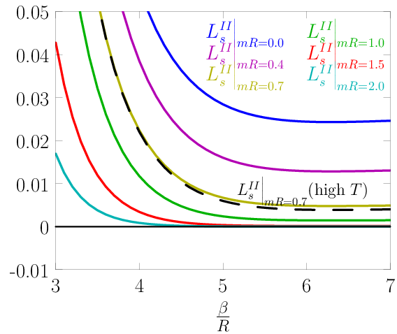
Figure 3: LL for scalars with various masses as a function of βR\frac{\beta}{R} including low temperature contributions. (Left) LsL_{s} calculated with scheme II-regularized Casimir energy where μ≡e−γE\mu\equiv e^{-\gamma_{E}}. (Right) LsL_{s} calculated with scheme I​III-regularized Casimir energy where μ≡12​m​R​exp⁡[2+m2​R24​(1+m2​R2)]\mu\equiv\frac{1}{2}mR\exp\left[\frac{2+m^{2}R^{2}}{4(1+m^{2}R^{2})}\right]. The dotted line corresponds to the high TT approximation of LsL_{s} for m​R=0.7mR=0.7.

Figure 3 (Left) shows LsIL_{s}^{I} in (75), referred to as LsI​(high​T)L_{s}^{I}({\rm high}~T), as a function of βR\frac{\beta}{R} for m​R=0.7mR=0.7 along with numerical calculations of LsIL_{s}^{I}, including the low temperature contributions in (63), for various m​RmR. It turns out that when regularization scheme II is used to obtain the Casimir energy, there exists a critical range 0.455∼<m​R∼<0.8640.455\raisebox{-2.15277pt}{$\ \stackrel{{\scriptstyle\textstyle<}}{{\textstyle\sim}}\ $}mR\raisebox{-2.15277pt}{$\ \stackrel{{\scriptstyle\textstyle<}}{{\textstyle\sim}}\ $}0.864 within which LsI<0L_{s}^{I}<0 for a range of βR\frac{\beta}{R}.

If regularization scheme II is used instead, with μ≡12​m​R​exp⁡[2+m2​R24​(1+m2​R2)]\mu\equiv\frac{1}{2}mR\exp\left[\frac{2+m^{2}R^{2}}{4(1+m^{2}R^{2})}\right], then the Casimir energy in (41) is used to obtain the partition function from (62) such that

log⁡ZsI​I≃dℛ{π4​R345​β3−m2​π2​R312​β+16πm3R3+12[m2R2log(1−e−2​π​m​R)−m​RπLi2(e−2​π​m​R)−12​π2Li3(e−2​π​m​R)]+β16​Rm4R4[−34+γE+log(m​β4​π)]+ξs(β/R,mR)}.\begin{split}\log Z_{s}^{II}\simeq&d_{{\cal R}}\Bigg\{\frac{\pi^{4}R^{3}}{45\beta^{3}}-\frac{m^{2}\pi^{2}R^{3}}{12\beta}+\frac{1}{6}\pi m^{3}R^{3}+\frac{1}{2}\bigg[m^{2}R^{2}\log\left(1-e^{-2\pi mR}\right)\\ &-\frac{mR}{\pi}{\rm Li}_{2}(e^{-2\pi mR})-\frac{1}{2\pi^{2}}{\rm Li}_{3}(e^{-2\pi mR})\bigg]\\ &+\frac{\beta}{16R}m^{4}R^{4}\left[-\frac{3}{4}+\gamma_{E}+\log\left(\frac{m\beta}{4\pi}\right)\right]+\xi_{s}(\beta/R,mR)\Bigg\}\,.\end{split} (79)

Using this in (6) gives

LsI​I≃Nsdℛ[2​π5​R415​β4−4​π4​R345​β3−π3​m2​R46​β2+π2​m2​R36​β−16πm3R3−18πm4R4(14+γE)−12​m2​R2​log⁡(1−e−2​π​m​R)+m​R2​π​Li2​(e−2​π​m​R)+14​π2​Li3​(e−2​π​m​R)+116​m4​R3​β+18πm4R4log(4​πm​β)+ξs′(β/R,mR)].\begin{split}L_{s}^{II}\simeq&N_{s}d_{{\cal R}}\bigg[\frac{2\pi^{5}R^{4}}{15\beta^{4}}-\frac{4\pi^{4}R^{3}}{45\beta^{3}}-\frac{\pi^{3}m^{2}R^{4}}{6\beta^{2}}+\frac{\pi^{2}m^{2}R^{3}}{6\beta}-\frac{1}{6}\pi m^{3}R^{3}-\frac{1}{8}\pi m^{4}R^{4}(\tfrac{1}{4}+\gamma_{E})\\ &-\frac{1}{2}m^{2}R^{2}\log\left(1-e^{-2\pi mR}\right)+\frac{mR}{2\pi}{\rm Li}_{2}(e^{-2\pi mR})+\frac{1}{4\pi^{2}}{\rm Li}_{3}(e^{-2\pi mR})+\frac{1}{16}m^{4}R^{3}\beta\\ &+\frac{1}{8}\pi m^{4}R^{4}\log\left(\frac{4\pi}{m\beta}\right)+\xi_{s}^{\prime}(\beta/R,mR)\bigg]\,.\end{split} (80)

The result is plotted in Figure 3 (Right) as a function of βR\frac{\beta}{R} for m​R=0.7mR=0.7 along with numerical calculations of the full result for various m​RmR including the low temperature contributions in (63). In contrast to LsIL_{s}^{I} it appears that LsI​I>0L_{s}^{II}>0 for all βR\frac{\beta}{R} regardless of the value of m​RmR. The difference between LsI​IL_{s}^{II} and LsIL_{s}^{I} is

LsI​I−LsI≃π​m4​R48​[−14−γE+log⁡2−log⁡(m​R)],\begin{split}L_{s}^{II}-L_{s}^{I}\simeq\frac{\pi m^{4}R^{4}}{8}\left[-\frac{1}{4}-\gamma_{E}+\log 2-\log\left(mR\right)\right]\,,\end{split} (81)

which is positive for m​R<2​e−14−γE≃0.875mR<2e^{-\frac{1}{4}-\gamma_{E}}\simeq 0.875, after which LI​I<LIL^{II}<L^{I}. This suggests that LsIL_{s}^{I} is only able to violate the Bekenstein bound when m​R∼<0.875mR\raisebox{-2.15277pt}{$\ \stackrel{{\scriptstyle\textstyle<}}{{\textstyle\sim}}\ $}0.875, which is satisfied by the range determined numerically, 0.455∼<m​R∼<0.8640.455\raisebox{-2.15277pt}{$\ \stackrel{{\scriptstyle\textstyle<}}{{\textstyle\sim}}\ $}mR\raisebox{-2.15277pt}{$\ \stackrel{{\scriptstyle\textstyle<}}{{\textstyle\sim}}\ $}0.864.

4.3 Fermions

The contribution to the partition function of NfN_{f} Weyl (Majorana) fermions of mass mm in representation ℛ{\cal R} is given by

log⁡Zf=−Nf​(Ξf+β​EC​a​s(f)),\begin{split}\log Z_{f}=-N_{f}(\Xi_{f}+\beta E_{Cas}^{(f)})\,,\end{split} (82)

where using (16), (17), (22), and setting θi=0\theta_{i}=0 gives

Ξf=2​dℛ​∑n=1∞(−1)nn​∑l=1∞l⁡(l+1)​e−n​βR​(l+12)2+m2​R2.\begin{split}\Xi_{f}=2d_{{\cal R}}\sum_{n=1}^{\infty}\frac{(-1)^{n}}{n}\sum_{l=1}^{\infty}l(l+1)e^{-n\frac{\beta}{R}\sqrt{(l+\frac{1}{2})^{2}+m^{2}R^{2}}}\,.\end{split} (83)

Applying the Mellin transform (29) the sum takes the form

Ξf=2​dℛ2​π​i​∫𝒞d​s​Gf​(s),\begin{split}\Xi_{f}=\frac{2d_{{\cal R}}}{2\pi i}\int_{{\cal C}}{\rm d}s\,G_{f}(s)\,,\end{split} (84)

where the integrand is given by

Gf​(s)≡Γ(s)(βR)−s∑n=1∞(−1)nns+1∑l=0∞l(l+1)[(l+12)2+m2R2]−s/2,=(−1+2−s)ζ(s+1)Γ(s)(βR)−s∑l=0∞[[(l+12)2+m2R2]1−s/2−(14+m2R2)[(l+12)2+m2R2]−s/2].\begin{split}G_{f}(s)\equiv&\Gamma(s)\left(\frac{\beta}{R}\right)^{-s}\sum_{n=1}^{\infty}\frac{(-1)^{n}}{n^{s+1}}\sum_{l=0}^{\infty}l(l+1)\left[\left(l+\tfrac{1}{2}\right)^{2}+m^{2}R^{2}\right]^{-s/2}\,,\\ =&(-1+2^{-s})\zeta(s+1)\Gamma(s)\left(\frac{\beta}{R}\right)^{-s}\sum_{l=0}^{\infty}\Bigg[\left[\left(l+\tfrac{1}{2}\right)^{2}+m^{2}R^{2}\right]^{1-s/2}\\ &-\left(\tfrac{1}{4}+m^{2}R^{2}\right)\left[\left(l+\tfrac{1}{2}\right)^{2}+m^{2}R^{2}\right]^{-s/2}\Bigg]\,.\end{split} (85)

4.3.1 Massless fermions

Refer to caption
Refer to caption
Figure 4: (Left) Comparison of the full Ξf​(all)\Xi_{f}({\rm all}) and the high temperature approximation Ξf​(high​T)\Xi_{f}({\rm high}~T) as a function of βR\frac{\beta}{R}. (Right) LfL_{f} as a function for βR\frac{\beta}{R} for theories with massless fermions in the deconfined phase using the full Ξf\Xi_{f}, labeled Lf​(all)L_{f}({\rm all}), and the high temperature approximation, labeled Lf​(high​T)L_{f}({\rm high}~T).

In the massless limit the integrand simplies to

Gf​(s)=(−1+2−s)​ζ​(s+1)​Γ​(s)​(βR)−s​[ζ⁡(s−2,12)−14​ζ​(s,12)].\begin{split}G_{f}(s)=(-1+2^{-s})\zeta(s+1)\Gamma(s)\left(\frac{\beta}{R}\right)^{-s}\left[\zeta(s-2,\tfrac{1}{2})-\frac{1}{4}\zeta(s,\tfrac{1}{2})\right]\,.\end{split} (86)

Collecting the non-zero residues at s=3,1,−1s=3,1,-1, the high temperature contribution from the closed contour integral takes the form

Ξf≃2​dℛ​[−7​π4​R3360​β3+π2​R48​β−17​β1920​R].\begin{split}\Xi_{f}\simeq&2d_{{\cal R}}\left[-\frac{7\pi^{4}R^{3}}{360\beta^{3}}+\frac{\pi^{2}R}{48\beta}-\frac{17\beta}{1920R}\right]\,.\end{split} (87)

This result is plotted in Figure 4 (Left) as a function of βR\frac{\beta}{R}, where it is referred to as Ξf​(high​T)\Xi_{f}({\rm high}~T), along with the direct numerical calculation of (83), referred to as Ξf​(all)\Xi_{f}({\rm all}), which includes the low temperature contributions. The partition function calculated from (82) using (87) and the Casimir energy in (43) is

log⁡Zf≃Nf​dℛ​[7​π4​R3180​β3−π2​R24​β].\begin{split}\log Z_{f}\simeq&N_{f}d_{{\cal R}}\left[\frac{7\pi^{4}R^{3}}{180\beta^{3}}-\frac{\pi^{2}R}{24\beta}\right]\,.\end{split} (88)

Using this in (6) gives

Lf≃Nf​dℛ​[7​π5​R430​β4−7​π4​R345​β3+112​(−π3​R2β2+π2​Rβ)],\begin{split}L_{f}\simeq&N_{f}d_{{\cal R}}\bigg[\frac{7\pi^{5}R^{4}}{30\beta^{4}}-\frac{7\pi^{4}R^{3}}{45\beta^{3}}+\frac{1}{12}\left(-\frac{\pi^{3}R^{2}}{\beta^{2}}+\frac{\pi^{2}R}{\beta}\right)\bigg]\,,\end{split} (89)

which is positive for all βR\frac{\beta}{R} and is plotted in Figure 4 (Right) and labeled Lf​(high​T)L_{f}({\rm high}~T), along with the numerical calculation of LfL_{f}, labeled Lf​(all)L_{f}({\rm all}), which includes low temperature contributions in (83). It appears that Lf​(all)>0L_{f}({\rm all})>0 for all βR\frac{\beta}{R} since it asymptotes quickly to Lf​(all)→β→∞2​π​R​EC​a​s(f)=17​π480​dℛ(f)≈0.111​dℛ(f)L_{f}({\rm all})\xrightarrow[\beta\rightarrow\infty]{}2\pi RE_{Cas}^{(f)}=\frac{17\pi}{480}d_{{\cal R}}^{(f)}\approx 0.111d_{{\cal R}}^{(f)}. The minimum of LfL_{f} in (89) is

Lf|βR=∞≃0.\begin{split}L_{f}\Big|_{\frac{\beta}{R}=\infty}\simeq 0\,.\end{split} (90)

4.3.2 Massive fermions

The sums over ll in (85) can be performed using (46) such that Gf​(s)G_{f}(s) simplifies to

Gf​(s)=(1−2s)(βR)−sζ(s+1)Γ(s+12){18(mR)1−s(m2R2−14(s−3))Γ(s−32)+∑n=1∞(−1)n[(s2−1)(π​nm​R)(s−3)/2Ks−32(2πnmR)−(14+m2R2)(π​nm​R)(s−1)/2Ks−12(2πnmR)]}.\begin{split}G_{f}(s)=&(1-2^{s})\left(\frac{\beta}{R}\right)^{-s}\zeta(s+1)\Gamma(\tfrac{s+1}{2})\bigg\{\frac{1}{8}(mR)^{1-s}\left(m^{2}R^{2}-\frac{1}{4}(s-3)\right)\Gamma(\tfrac{s-3}{2})\\ &+\sum_{n=1}^{\infty}(-1)^{n}\bigg[(\tfrac{s}{2}-1)\left(\frac{\pi n}{mR}\right)^{(s-3)/2}K_{\frac{s-3}{2}}(2\pi nmR)\\ &\hskip 68.2866pt-(\tfrac{1}{4}+m^{2}R^{2})\left(\frac{\pi n}{mR}\right)^{(s-1)/2}K_{\frac{s-1}{2}}(2\pi nmR)\bigg]\bigg\}\,.\end{split} (91)

Adding an arc at infinity in the left half complex ss-plane to close the contour in (84) around the poles in Gf​(s)G_{f}(s) results in non-zero residues for s=3,1,−1,−3,−5,…s=3,1,-1,-3,-5,.... Collecting these results in

Ξf≃ 2dℛ{−7​π4​R3360​β3+π2​R24​β(m2R2+12)+β2​R∑k=1∞(−1)k[32m2​R2π2​k2K2(2πkmR)+(m2R2+14)m​Rπ​kK1(2πkmR)]+β8​Rm2R2[−14+12γE+18(4γE−3)m2R2+12(1+m2R2)log(m​βπ)]}+dℛ​ξf​(m​R,βR),\begin{split}\Xi_{f}\simeq&\,2d_{{\cal R}}\bigg\{-\frac{7\pi^{4}R^{3}}{360\beta^{3}}+\frac{\pi^{2}R}{24\beta}\left(m^{2}R^{2}+\tfrac{1}{2}\right)\\ &\,+\frac{\beta}{2R}\sum_{k=1}^{\infty}(-1)^{k}\left[\frac{3}{2}\frac{m^{2}R^{2}}{\pi^{2}k^{2}}{\rm K}_{2}(2\pi kmR)+(m^{2}R^{2}+\tfrac{1}{4})\frac{mR}{\pi k}{\rm K}_{1}(2\pi kmR)\right]\\ &\,+\frac{\beta}{8R}m^{2}R^{2}\bigg[-\frac{1}{4}+\frac{1}{2}\gamma_{E}+\frac{1}{8}(4\gamma_{E}-3)m^{2}R^{2}+\frac{1}{2}(1+m^{2}R^{2})\log\left(\tfrac{m\beta}{\pi}\right)\bigg]\bigg\}\\ &\,+d_{{\cal R}}\xi_{f}(mR,\tfrac{\beta}{R})\,,\end{split} (92)

where ξf​(m​R,βR)=𝒪​(βR)3​𝒪​(m​R)4\xi_{f}(mR,\frac{\beta}{R})={\cal O}\left(\frac{\beta}{R}\right)^{3}{\cal O}(mR)^{4} and takes the form

ξf​(m​R,βR)=m2​β​R8​∑n=1∞(−1)n​Γ⁡(2​n+1)​ζ​(2​n+1)Γ⁡(n+3)​Γ​(n+1)​(m​β4​π)2​n​(22​n+1−1)​(2​m2​R2+2+n).\begin{split}&\xi_{f}\left(mR,\tfrac{\beta}{R}\right)\\ &=\frac{m^{2}\beta R}{8}\sum_{n=1}^{\infty}(-1)^{n}\frac{\Gamma(2n+1)\zeta(2n+1)}{\Gamma(n+3)\Gamma(n+1)}\left(\frac{m\beta}{4\pi}\right)^{2n}\left(2^{2n+1}-1\right)(2m^{2}R^{2}+2+n)\,.\end{split} (93)

The contribution to the partition function resulting from the second line in (92) cancels with the Casimir contribution, and, for regularization scheme II, so does part of the third line. The remaining high-temperature partition function, first assuming scheme II regularization of the Casimir energy, is obtained from (82) using the Casimir energy in (52), which gives

log⁡ZfI≃Nfdℛ[7​π4​R3180​β3−π2​R12​β(m2R2+12)+β8​Rm2R2(1+m2R2)(1+log(π​R2​β))−ξf(mR,βR)].\begin{split}\log Z_{f}^{I}\simeq&N_{f}d_{{\cal R}}\bigg[\frac{7\pi^{4}R^{3}}{180\beta^{3}}-\frac{\pi^{2}R}{12\beta}(m^{2}R^{2}+\tfrac{1}{2})+\frac{\beta}{8R}m^{2}R^{2}(1+m^{2}R^{2})\left(1+\log\left(\frac{\pi R}{2\beta}\right)\right)\\ &-\xi_{f}\left(mR,\tfrac{\beta}{R}\right)\bigg]\,.\end{split} (94)

It is now possible to consider whether the Bekenstein bound is satisfied. Calculating LL from (6) gives

LfI≃Nfdℛ[7​π5​R430​β4−7​π4​R345​β3+112(1+2m2R2)(−π3​R2β2+π2​Rβ)+18m2R2(1+m2R2)(−βR+2πlog(2​βπ​R))+ξf′(mR,βR)],\begin{split}L_{f}^{I}\simeq&N_{f}d_{{\cal R}}\bigg[\frac{7\pi^{5}R^{4}}{30\beta^{4}}-\frac{7\pi^{4}R^{3}}{45\beta^{3}}+\frac{1}{12}\left(1+2m^{2}R^{2}\right)\left(-\frac{\pi^{3}R^{2}}{\beta^{2}}+\frac{\pi^{2}R}{\beta}\right)\\ &+\frac{1}{8}m^{2}R^{2}\left(1+m^{2}R^{2}\right)\left(-\frac{\beta}{R}+2\pi\log\left(\frac{2\beta}{\pi R}\right)\right)+\xi_{f}^{\prime}\left(mR,\tfrac{\beta}{R}\right)\bigg]\,,\end{split} (95)

where ξf′​(m​R,βR)=𝒪​(βR)2​𝒪​(m​R)4\xi_{f}^{\prime}(mR,\frac{\beta}{R})={\cal O}\left(\frac{\beta}{R}\right)^{2}{\cal O}(mR)^{4} and takes the form

ξf′​(m​R,βR)=m2​R4∑n=1∞[(−1)nΓ⁡(2​n+1)​ζ​(2​n+1)Γ⁡(n+3)​Γ​(n+1)(m​β4​π)2​n(22​n+1−1)×(2m2R2+2+n)[(β−2πR)n−πR]].\begin{split}\xi_{f}^{\prime}\left(mR,\tfrac{\beta}{R}\right)=&\frac{m^{2}R}{4}\sum_{n=1}^{\infty}\bigg[(-1)^{n}\frac{\Gamma(2n+1)\zeta(2n+1)}{\Gamma(n+3)\Gamma(n+1)}\left(\frac{m\beta}{4\pi}\right)^{2n}\left(2^{2n+1}-1\right)\\ &\hskip 56.9055pt\times(2m^{2}R^{2}+2+n)\left[(\beta-2\pi R)n-\pi R\right]\bigg]\,.\end{split} (96)

To determine the behavior of LfL_{f} when m​R≠0mR\neq 0 it is necessary to determine if the sum in ξf′​(m​R,βR)\xi_{f}^{\prime}(mR,\tfrac{\beta}{R}) converges. To this end it is helpful to consider the large nn limit

limn→∞ξf′​(m​R,βR)=m2​R2​n3/2​π​(−1)n​(m​βπ)2​n​[(β−2​π​R)​n−π​R].\begin{split}\lim_{n\rightarrow\infty}\xi_{f}^{\prime}\left(mR,\tfrac{\beta}{R}\right)=\frac{m^{2}R}{2n^{3/2}\sqrt{\pi}}(-1)^{n}\left(\frac{m\beta}{\pi}\right)^{2n}\left[(\beta-2\pi R)n-\pi R\right]\,.\end{split} (97)

Setting aside the constants the relevant limits are

(−1)nn3/2​(m​βπ)2​n​[(β−2​π​R)​n−π​R]→n→∞0,if​m​β≤π,→n→∞±∞,if​m​β>π.\begin{split}\frac{(-1)^{n}}{n^{3/2}}\left(\frac{m\beta}{\pi}\right)^{2n}\left[(\beta-2\pi R)n-\pi R\right]&\xrightarrow[n\rightarrow\infty]{}\hskip 28.45274pt0,\hskip 28.45274pt{\rm if}~m\beta\leq\pi\,,\\ &\xrightarrow[n\rightarrow\infty]{}\hskip 14.22636pt\pm\infty,\hskip 28.45274pt{\rm if}~m\beta>\pi\,.\end{split} (98)

Therefore the sum in ξf′​(m​R,βR)\xi_{f}^{\prime}\left(mR,\tfrac{\beta}{R}\right) converges for m​β≤πm\beta\leq\pi and can be truncated as an approximation. However, when m​β>πm\beta>\pi the sum diverges to ±∞\pm\infty depending on whether it is truncated at an even or odd number, and ξf′\xi_{f}^{\prime} must be regularized.

Refer to caption
Refer to caption
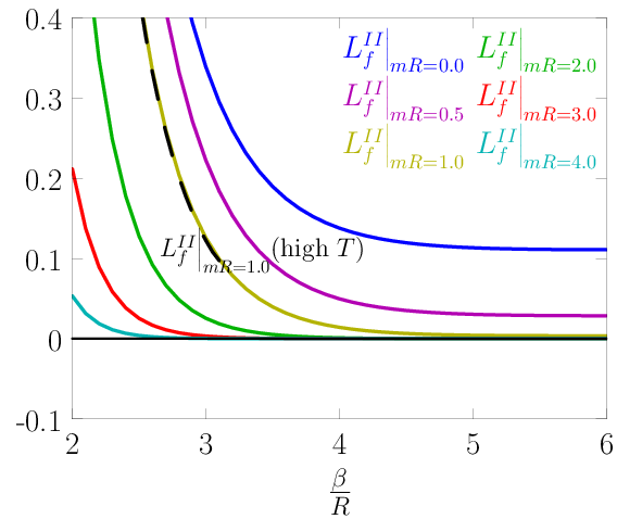
Figure 5: LL for fermions with various masses as a function of βR\frac{\beta}{R} including the low temperature contributions. (Left) LfL_{f} calculated including scheme II-regularized Casimir energy with μ≡e−γE\mu\equiv e^{-\gamma_{E}}. (Right) LfL_{f} calculated including scheme I​III-regularized Casimir energy with μ≡12​m​R​exp⁡[2+m2​R24​(1+m2​R2)]\mu\equiv\frac{1}{2}mR\exp\left[\frac{2+m^{2}R^{2}}{4(1+m^{2}R^{2})}\right]. The dotted line gives the high TT results for LfL_{f} with m​R=1.0mR=1.0.

Figure 5 (Left) shows LfIL_{f}^{I} in (95), labeled LfI​(high​T)L_{f}^{I}({\rm high}~T), as a function of βR\frac{\beta}{R} for m​R=1.0mR=1.0, along with LfIL_{f}^{I} computed numerically including the low temperature contributions in (83) for various m​RmR. Using regularization scheme II, with μ≡e−γE\mu\equiv e^{-\gamma_{E}}, to obtain the Casimir energy, taking m​R∼>0.757mR\raisebox{-2.15277pt}{$\ \stackrel{{\scriptstyle\textstyle>}}{{\textstyle\sim}}\ $}0.757 results in violation of the Bekenstein bound above a certain critical value of βR\frac{\beta}{R}, which decreases with increasing m​RmR.

Considering regularization scheme I​III, with μ≡12​m​R​exp⁡[2+m2​R24​(1+m2​R2)]\mu\equiv\frac{1}{2}mR\exp\left[\frac{2+m^{2}R^{2}}{4(1+m^{2}R^{2})}\right], the Casimir energy in (53) is used with the result (92) to obtain the partition function via (82), resulting in

log⁡ZfI​I≃Nfdℛ[7​π4​R3180​β3−π2​R12​β(m2R2+12)+β8​Rm2R2(12−γE+m2R2(34−γE))+β8​Rm2R2(1+m2R2)log(πm​β)−ξf(mR,βR)].\begin{split}\log Z_{f}^{II}\simeq&N_{f}d_{{\cal R}}\bigg[\frac{7\pi^{4}R^{3}}{180\beta^{3}}-\frac{\pi^{2}R}{12\beta}(m^{2}R^{2}+\tfrac{1}{2})+\frac{\beta}{8R}m^{2}R^{2}\left(\tfrac{1}{2}-\gamma_{E}+m^{2}R^{2}\left(\tfrac{3}{4}-\gamma_{E}\right)\right)\\ &+\frac{\beta}{8R}m^{2}R^{2}\left(1+m^{2}R^{2}\right)\log\left(\frac{\pi}{m\beta}\right)-\xi_{f}\left(mR,\tfrac{\beta}{R}\right)\bigg]\,.\end{split} (99)

Using this in (6) gives

LfI​I≃Nfdℛ[7​π5​R430​β4−7​π4​R345​β3+112(1+2m2R2)(−π3​R2β2+π2​Rβ)+18​π​m2​R2​(1+12​m2​R2)+14​π​γE​m2​R2​(1+m2​R2)+18m2R2(1+m2R2)(−βR+2πlog(m​βπ))+ξf′(mR,βR)].\begin{split}L_{f}^{II}\simeq&N_{f}d_{{\cal R}}\bigg[\frac{7\pi^{5}R^{4}}{30\beta^{4}}-\frac{7\pi^{4}R^{3}}{45\beta^{3}}+\frac{1}{12}\left(1+2m^{2}R^{2}\right)\left(-\frac{\pi^{3}R^{2}}{\beta^{2}}+\frac{\pi^{2}R}{\beta}\right)\\ &+\frac{1}{8}\pi m^{2}R^{2}\left(1+\frac{1}{2}m^{2}R^{2}\right)+\frac{1}{4}\pi\gamma_{E}m^{2}R^{2}\left(1+m^{2}R^{2}\right)\\ &+\frac{1}{8}m^{2}R^{2}\left(1+m^{2}R^{2}\right)\left(-\frac{\beta}{R}+2\pi\log\left(\frac{m\beta}{\pi}\right)\right)+\xi_{f}^{\prime}\left(mR,\tfrac{\beta}{R}\right)\bigg]\,.\end{split} (100)

Figure 5 (Right) shows this result, labeled LfI​I​(high​T)L_{f}^{II}({\rm high}~T), for m​R=1.0mR=1.0, along with numerical calculations of LfI​IL_{f}^{II} including the low temperature contributions from (83) for various m​RmR. Thus, when the Casimir energy is obtained using regularization scheme I​III, such that EC​a​s>0E_{Cas}>0 for all m​RmR, the Bekenstein bound appears to be satisfied for all βR\frac{\beta}{R}, for any m​RmR.

The difference between LI​IL^{II} and LIL^{I} is

LI​I−LI≃π4​m2​R2​[12+γE+log⁡(m​R2)]+π4​m4​R4​[14+γE+log⁡(m​R2)],\begin{split}L^{II}-L^{I}\simeq\frac{\pi}{4}m^{2}R^{2}\left[\frac{1}{2}+\gamma_{E}+\log\left(\frac{mR}{2}\right)\right]+\frac{\pi}{4}m^{4}R^{4}\left[\frac{1}{4}+\gamma_{E}+\log\left(\frac{mR}{2}\right)\right]\,,\end{split} (101)

which is positive for m​R∼>0.745mR\raisebox{-2.15277pt}{$\ \stackrel{{\scriptstyle\textstyle>}}{{\textstyle\sim}}\ $}0.745. This reveals that, assuming LfI​I>0L_{f}^{II}>0, it is possible for LfIL_{f}^{I} to violate the bound for masses above this value, and supports the numerical result that LfI<0L_{f}^{I}<0 for m​R∼>0.757mR\raisebox{-2.15277pt}{$\ \stackrel{{\scriptstyle\textstyle>}}{{\textstyle\sim}}\ $}0.757.

5 Low temperature partition functions (confined phase)

Another interesting question is whether the Bekenstein bound continues to hold if the temperature is decreased and the theory undergoes a phase transition from the deconfined phase to the confined phase. During the transition the eigenvalues of the Polyakov line go from being clumped with θi=0\theta_{i}=0 to being uniformly distributed around the unit circle. For U⁡(Nc)U(N_{c}) or S​U​(Nc)SU(N_{c}) theories with odd NcN_{c} the Polyakov line angles in the confined phase take the form θ={0,2​πNc,4​πNc,…,(Nc−1)​πNc}\theta=\{0,\frac{2\pi}{N_{c}},\frac{4\pi}{N_{c}},...,\frac{(N_{c}-1)\pi}{N_{c}}\} (for NcN_{c} even the angles are shifted by πNc\frac{\pi}{N_{c}}). Taking the trace of the Polyakov line with the angles evenly distributed around the unit circle results in 𝒫n(ℱ)=∑i=1Ncei​n​θi=0{\mathscr{P}}_{n}^{({\cal F})}=\sum_{i=1}^{N_{c}}e^{in\theta_{i}}=0.

For U⁡(Nc)U(N_{c}) theories, or S​U​(Nc)SU(N_{c}) theories with large NcN_{c}, containing only fundamental and/or adjoint matter, 𝒫n(ℱ)=0{\mathscr{P}}_{n}^{({\cal F})}=0 implies that the zero-point contribution to the partition function is all that remains. Since the Casimir energy is always positive for theories with massless matter then the Bekenstein bound is trivially satisfied in the confined phase since L=−2​π​Rβ​log⁡Z=2​π​R​EC​a​sL=-\frac{2\pi R}{\beta}\log Z=2\pi RE_{Cas}. For the same reason it is also satisfied for massive matter when the Casimir energy is regularized according to scheme I​III. However, for massive matter with the Casimir energy regularized according to scheme II there is a range of m​RmR which results in EC​a​s<0E_{Cas}<0 and causes the Bekenstein bound to be violated.

The only remaining case where it is not clear if the Bekenstein bound holds is for S​U​(Nc)SU(N_{c}) theories in the confined phase and with NcN_{c} not large. In the next section we consider what happens in pure Yang-Mills theory.

5.1 S​U​(Nc)SU(N_{c}) Yang-Mills theory with finite NcN_{c}

For S​U​(Nc)SU(N_{c}) Yang-Mills theory in the confined phase ∑i,j=1Nccos⁡(n⁡(θi−θj))=0\sum_{i,j=1}^{N_{c}}\cos(n(\theta_{i}-\theta_{j}))=0 and it is only necessary to keep the −1-1 contribution from trace over the Polyakov lines in the adjoint representation. The vector sum takes the form

ΞS​U​(N)Y​M=−2∑n=1∞1n∑l=1∞l(l+2)e−n​βR​(l+1).\begin{split}\Xi_{SU(N)}^{YM}=-2\sum_{n=1}^{\infty}\frac{1}{n}\sum_{l=1}^{\infty}l(l+2)e^{-n\frac{\beta}{R}(l+1)}\,.\end{split} (102)

In the limit of large βR\frac{\beta}{R} where the uniform distribution is preferred it is possible to approximate the sum over nn by its n=1n=1 term,

ΞS​U​(N)Y​M≃−2∑l=1∞l(l+2)e−n​βR​(l+1),=−6e−2β/R+2e−3β/R(1−e−β/R)3.\begin{split}\Xi_{SU(N)}^{YM}&\simeq-2\sum_{l=1}^{\infty}l(l+2)e^{-n\frac{\beta}{R}(l+1)}\,,\\ &=\frac{-6e^{-2\beta/R}+2e^{-3\beta/R}}{(1-e^{-\beta/R})^{3}}\,.\end{split} (103)

Adding the Casimir contribution −β​EC​a​s(v)-\beta E_{Cas}^{(v)} from (54) the partition function is

log⁡Z≃−6e−2β/R+2e−3β/R(1−e−β/R)3−(Nc2−1)​11​β120​R.\begin{split}\log Z\simeq\frac{-6e^{-2\beta/R}+2e^{-3\beta/R}}{(1-e^{-\beta/R})^{3}}-(N_{c}^{2}-1)\frac{11\beta}{120R}\,.\end{split} (104)

Plugging this into (6) results in

L=1(1−e−β/R)4[(Nc2−1)(−11​π60+11πe−β/R15)+(−6+251​π10−11​Nc2​π10)e−2β/R+((Nc2−1)11​π15+8)e−3β/R+(−(Nc2−1)11​π60−2)e−4β/R−12βe−2β/RR].\begin{split}L=&\frac{1}{(1-e^{-\beta/R})^{4}}\bigg[(N_{c}^{2}-1)\left(-\frac{11\pi}{60}+\frac{11\pi e^{-\beta/R}}{15}\right)+\left(-6+\frac{251\pi}{10}-\frac{11N_{c}^{2}\pi}{10}\right)e^{-2\beta/R}\\ &+\left((N_{c}^{2}-1)\frac{11\pi}{15}+8\right)e^{-3\beta/R}+\left(-(N_{c}^{2}-1)\frac{11\pi}{60}-2\right)e^{-4\beta/R}-\frac{12\beta e^{-2\beta/R}}{R}\bigg]\,.\end{split} (105)

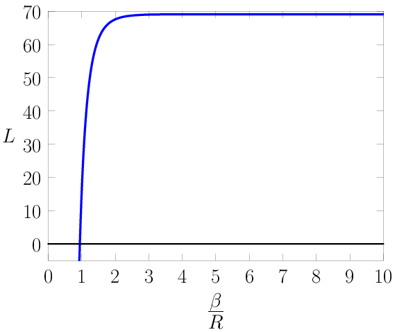
As βR→0\frac{\beta}{R}\rightarrow 0 it is clear that L<0L<0 and as βR→∞\frac{\beta}{R}\rightarrow\infty that L>0L>0. At some intermediate βR\frac{\beta}{R} is the transition point L=0L=0. Figure 6 (Left) shows LL as a function of βR\frac{\beta}{R} for Nc=11N_{c}=11 and Figure 6 (Right) shows the L=0L=0 transition point as a function of βR\frac{\beta}{R} for odd NcN_{c} from 33 to 3939. For Nc=3N_{c}=3, the L=0L=0 transition point occurs at βR≈1.637\frac{\beta}{R}\approx 1.637, however it should be noted that the saddle point method used to obtain (14) is at best a rough approximation when NcN_{c} is not large. Keeping more terms in the sum over nn in (102) makes a negligible difference. The deconfinement confinement transition occurs at βR≈1.317\frac{\beta}{R}\approx 1.317 [10] for weak-coupling Yang-Mills theory at large NcN_{c}, however the transition is smeared out when considering finite NcN_{c}. Therefore it is not clear in the case of Nc=3N_{c}=3 if the L=0L=0 point is within the confined phase or not. However, in the Nc→∞N_{c}\rightarrow\infty limit the L=0L=0 point gets pushed to βR=0\frac{\beta}{R}=0, such that L>0L>0 for all βR>0\frac{\beta}{R}>0.

Refer to caption
Refer to caption
Figure 6: LL for theories with massless vectors in the confined phase. (Left) LL vs. βR\frac{\beta}{R} with Nc=11N_{c}=11. (Right) Critical L=0L=0 line as a function of βR\frac{\beta}{R} and odd NcN_{c} from 33 to 3939. The dashed line indicates the temperature of the deconfinement transition for Nc=∞N_{c}=\infty Yang-Mills theory.

6 Verlinde bound

It is straightforward to use the same techniques applied to the Bekenstein bound analysis to test the Verlinde bound [17], which takes the form

S≤2​π3​R​E,\begin{split}S\leq\frac{2\pi}{3}RE\,,\end{split} (106)

for conformal theories on S1×S3S^{1}\times S^{3}. For 𝒩=4{\cal N}=4 SYM theory which has 66 real scalars, 1 vector, and 44 Weyl fermions, the relevant inequality is

6​LV​e​r(s)+LV​e​r(v)+4​LV​e​r(f)≥0,\begin{split}6L_{Ver}^{(s)}+L_{Ver}^{(v)}+4L_{Ver}^{(f)}\geq 0\,,\end{split} (107)

where LV​e​r=(β−2​π​R3)​∂∂β​log⁡Z−log⁡ZL_{Ver}=\left(\beta-\frac{2\pi R}{3}\right)\frac{\partial}{\partial\beta}\log Z-\log Z, and ZZ is the partition function (including the Casimir contribution) of the massless scalars, vectors, or fermions. Using the high temperature expansions for the partition functions from the previous sections

LV​e​r(s)≃2​π5​R445​β4−4​π4​R345​β3+14​π2​ζ​(3),LV​e​r(v)≃4​π5​R445​β4−8​π4​R345​β3−2​π3​R29​β2+2​π​R3​β​(π+1)+12​π2​ζ​(3)−1+log⁡(β2​π​R),LV​e​r(f)≃7​π5​R490​β4−7​π4​R345​β3−π3​R236​β2+π2​R12​β.\begin{split}L_{Ver}^{(s)}&\simeq\frac{2\pi^{5}R^{4}}{45\beta^{4}}-\frac{4\pi^{4}R^{3}}{45\beta^{3}}+\frac{1}{4\pi^{2}}\zeta(3)\,,\\ L_{Ver}^{(v)}&\simeq\frac{4\pi^{5}R^{4}}{45\beta^{4}}-\frac{8\pi^{4}R^{3}}{45\beta^{3}}-\frac{2\pi^{3}R^{2}}{9\beta^{2}}+\frac{2\pi R}{3\beta}(\pi+1)+\frac{1}{2\pi^{2}}\zeta(3)-1+\log\left(\frac{\beta}{2\pi R}\right)\,,\\ L_{Ver}^{(f)}&\simeq\frac{7\pi^{5}R^{4}}{90\beta^{4}}-\frac{7\pi^{4}R^{3}}{45\beta^{3}}-\frac{\pi^{3}R^{2}}{36\beta^{2}}+\frac{\pi^{2}R}{12\beta}\,.\end{split} (108)

Thus the inequality in (107) takes the form

2​π5​R43​β4−4​π4​R33​β3−π3​R23​β2+π​Rβ​(23+π)+2π2​ζ​(3)−1+log⁡(β2​π​R)≥0,\begin{split}\frac{2\pi^{5}R^{4}}{3\beta^{4}}-\frac{4\pi^{4}R^{3}}{3\beta^{3}}-\frac{\pi^{3}R^{2}}{3\beta^{2}}+\frac{\pi R}{\beta}(\tfrac{2}{3}+\pi)+\frac{2}{\pi^{2}}\zeta(3)-1+\log\left(\frac{\beta}{2\pi R}\right)\geq 0\,,\end{split} (109)

which means that L>0L>0 for βR∼<1.648\frac{\beta}{R}\raisebox{-2.15277pt}{$\ \stackrel{{\scriptstyle\textstyle<}}{{\textstyle\sim}}\ $}1.648. Since this value is in the regime where the high temperature approximation is very good calculating LV​e​r(x)L_{Ver}^{(x)} in (108) while including the low temperature corrections makes a negligible difference. We have checked this numerically. Note that the deconfinement-confinement transition at zero ’t Hooft coupling occurs at βR≈2.634\frac{\beta}{R}\approx 2.634 [10], and the corresponding strong coupling Hawking-Page transition occurs at βR=2​π3≈2.094\frac{\beta}{R}=\frac{2\pi}{3}\approx 2.094 [18, 19]. Either way, it appears that as βR\frac{\beta}{R} is increased, the weakly coupled theory violates the bound before the transition takes place. It is however important to recall the Vandermonde contribution LV​d​m≃d𝒜​(log⁡Λ+γE)L_{Vdm}\simeq d_{{\cal A}}(\log\Lambda+\gamma_{E}), which we dropped at the end of Section 2. It is possible that this contribution is sufficient to prevent violation of the Verlinde bound. The θi\theta_{i}-dependence, which is relevant near a phase transition, would need to be properly accounted for to be sure.

7 Conclusions

Using the approach in [9, 2] we have calculated the high temperature partition functions for gauge theories with massless vectors, scalars, and/or fermions, and for gauge theories with massive scalars and/or fermions, at zero ’t Hooft coupling on S1×S3S^{1}\times S^{3}, in the deconfined phase. From these results, and from numerical results including the low temperature contributions, the Bekenstein entropy bound was determined to hold at all βR\frac{\beta}{R} for theories with massless deconfined matter. This was also determined to be true for theories with massive scalars or fermions regularized using scheme I​III to obtain the Casimir energy, with regularization parameter μ\mu fixed to satisfy the constraint EC​a​s→0E_{Cas}\rightarrow 0 as m​R→∞mR\rightarrow\infty. When the Casimir energy was instead regularized using scheme II, which fixes μ\mu to match the zeta function result with the cutoff method result, then for both scalars and fermions we found a range of m​R≠0mR\neq 0 for which the Bekenstein bound was violated for a range of βR\frac{\beta}{R}.

Since it is clear that the Casimir energy must be positive in order for the Bekenstein bound to hold all the way into the low temperature regime then only our scheme I​III results could be expected to hold at all temperatures, and the fact that they appear to hold regardless of m​RmR is consistent with Bekenstein’s conjecture. What is yet unclear is which regularization procedure gives the correct, scheme-independent Casimir energy for theories with massive scalar or fermionic matter. If it is scheme II that gives the correct results then for theories with scalars or fermions of sufficiently low m​RmR Bekenstein’s bound still appears to hold at all temperatures.

We also considered matter in the confined phase to determine if the Bekenstein bound still holds when the theory undergoes a phase transition. In the confined phase the Trℛ​ei​n​θ{\rm Tr}_{{\cal R}}e^{in\theta}-dependent contributions to the partition function vanish in the case of U⁡(Nc)U(N_{c}) theories or S​U​(Nc)SU(N_{c}) theories at large NcN_{c} when the matter is in the adjoint and fundamental representations. The only case where it is unclear if the Bekenstein bound holds in the confined phase is for S​U​(Nc)SU(N_{c}) theories with NcN_{c} not large. It might be possible to check this numerically by performing the integrals over the θi\theta_{i} directly rather than using the saddle point approximation to get from the action to the partition function.

With regard to the Verlinde bound we found, in agreement with [2], that it is still violated for sufficiently large βR\frac{\beta}{R} before the deconfinement-confinement transition takes place, when considering 𝒩=4{\cal N}=4 SYM as a free theory. However, for the S​U​(Nc)SU(N_{c}) theory at zero ’t Hooft coupling, the Vandermonde contribution could be sufficient to prevent violation of the bound, but the θi\theta_{i}-dependence of the partition function near the transition temperature would need to be included to be sure.

8 Acknowledgements

We would like to thank Jan Rosseel for many useful conversations, for looking at the manuscript, and for checking some of the results. We would also like to thank Jose Barbon for helpful discussions regarding the physical relevance of the Bekenstein bound. The research of JCM is supported by the Stichting voor Fundamenteel Onderzoek der Materie (FOM).

References

  • [1] J. D. Bekenstein, Phys. Rev. D 23 (1981) 287.
  • [2] D. Kutasov, F. Larsen, JHEP 0101 (2001) 001. [hep-th/0009244].
  • [3] D. Klemm, A. C. Petkou and G. Siopsis, Nucl. Phys. B 601 (2001) 380 [hep-th/0101076].
  • [4] J. S. Dowker, Class. Quant. Grav. 20 (2003) L105 [hep-th/0203026].
  • [5] I. H. Brevik, K. A. Milton and S. D. Odintsov, Annals Phys. 302 (2002) 120 [hep-th/0202048].
  • [6] I. H. Brevik, K. A. Milton and S. D. Odintsov, hep-th/0210286.
  • [7] E. Elizalde and A. C. Tort, Phys. Rev. D 67 (2003) 124014 [arXiv:hep-th/0302155].
  • [8] G. W. Gibbons, M. J. Perry and C. N. Pope, Phys. Rev. D 74 (2006) 084009 [hep-th/0606186].
  • [9] J. L. Cardy, Nucl. Phys. B 366 (1991) 403.
  • [10] O. Aharony, J. Marsano, S. Minwalla, K. Papadodimas, M. Van Raamsdonk, Adv. Theor. Math. Phys. 8 (2004) 603-696. [hep-th/0310285].
  • [11] S. C. Lim and L. P. Teo, Annals Phys. 324 (2009) 1676 [arXiv:0807.3613 [hep-th]].
  • [12] E. Elizalde, A. C. Tort, [hep-th/0311114].
  • [13] S. Blau, M. Visser, A. Wipf, Nucl. Phys. B310 (1988) 163. [arXiv:0906.2817 [hep-th]].
  • [14] E. Elizalde, “Ten physical applications of spectral zeta functions,” Lect. Notes Phys. M35 (1995) 1-224.
  • [15] M. Bordag, U. Mohideen, V. M. Mostepanenko, Phys. Rept. 353 (2001) 1-205. [quant-ph/0106045].
  • [16] E. Elizalde and A. Romeo, Phys. Rev. D 40 (1989) 436.
  • [17] E. P. Verlinde, hep-th/0008140.
  • [18] S. W. Hawking and D. N. Page, Commun. Math. Phys. 87 (1983) 577.
  • [19] E. Witten, Adv. Theor. Math. Phys. 2 (1998) 505 [hep-th/9803131].