A locally minimal, but not globally minimal bridge position of a knotThanks: The first author is partially supported by Grant-in-Aid for Scientific Research (C) (No. 23540105), The Ministry of Education, Culture, Sports, Science and Technology, Japan
Abstract.
We give a locally minimal, but not globally minimal bridge position of a knot, that is, an unstabilized, nonminimal bridge position of a knot. It implies that a bridge position cannot always be simplified so that the bridge number monotonically decreases to the minimal.
Key words and phrases:
knot, bridge position, stabilization2010 Mathematics Subject Classification
57M251. Introduction
A knot is an equivalence class of embeddings of the circle into the 3-sphere , where two embeddings are said to be equivalent if an ambient isotopy of deforms one to the other. In knot theory, it is a fundamental and important problem to determine whether given two representatives of knots are equivalent, and furthermore to describe how one can be deformed to the other. In particular, a simplification to a “minimal position” is of great interest.
Let be the standard height function, that is, the restriction of to . A Morse position of a knot is a representative such that is disjoint from the poles of and the critical points of are all non-degenerate and have pairwise distinct values. Since is a circle, there are the same number of local maxima and local minima.
In [19], Schubert introduced the notion of bridge position and bridge number for knots. A bridge position of is a Morse position where all the local maxima are above all the local minima with respect to . A level -sphere separating the local maxima from the local minima is called a bridge sphere of . If intersects in points, then is called an -bridge position and is called the bridge number of . The minimum of the bridge number over all bridge positions of is called the bridge number of . A knot with the bridge number is called an -bridge knot. The bridge number is a fundamental geometric invariant of knots as well as the crossing number.
In [6], Gabai introduced the notion of width for knots. Suppose that is a Morse position of a knot , let be the critical levels of such that for , and choose regular levels of so that . The width of is defined as , and the width of is the minimum of the width over all Morse positions of .
Two Morse positions of a knot are isotopic if an ambient isotopy of deforms one to the other keeping it a Morse position except for exchanging two levels of local maxima or two levels of local minima. Such an isotopy preserves the width of a Morse position and the bridge number of a bridge position. The following two types of moves change the isotopy class of a Morse position.
Suppose that is a Morse position of a knot and let as above. We say that the level 2-sphere is thick if is a locally minimal level of and is a locally maximal level of , and that is thin if is a locally maximal level and is a locally minimal level. A strict upper (resp. lower) disk for a thick sphere is a disk such that the interior of does not intersect with and any thin sphere, the interior of contains no critical points with respect to , and consists of a subarc of and an arc in . Note that the arc has exactly one local maximum (resp. minimum). First suppose that there exist a strict upper disk and a strict lower disk for a thick sphere such that consists of a single point of . Then can be isotoped along and to cancel the local maximum in and the local minimum in . In [21], Schultens called this move a Type I move. The inverse operation of a Type I move is called a stabilization ([2], [12]) or a perturbation ([18], [23]) and the resultant position is said to be stabilized or perturbed. Next suppose that there exist a strict upper disk and a strict lower disk for a thick sphere such that . Then can be isotoped along and to exchange the two levels of the local maximum in and the local minimum in . Schultens ([21]) called this move a Type II move.


The following are fundamental theorems for bridge positions and Morse positions which correspond to Reidemeister’s theorem ([16], [1]) for knot diagrams.
Theorem 1.1 ([2], [7]).
Two knots are equivalent if and only if their two bridge positions can be related by a sequence of Type I moves and the inverse operations up to isotopy.
Theorem 1.2 ([21]).
Two knots are equivalent if and only if their two Morse positions can be related by a sequence of Type I and Type II moves and the inverse operations up to isotopy.
We say that a bridge position of a knot is globally minimal if it realizes the bridge number of , and a bridge position is locally minimal if it does not admit a Type I move. Similarly, we say that a Morse position of a knot is globally minimal if it realizes the width of , and a Morse position is locally minimal if it does not admit a Type I move nor a Type II move. Note that if a bridge (resp. Morse) position of a knot is globally minimal, then it is locally minimal. Otal (later Hayashi–Shimokawa, the first author) proved the converse for bridge positions of the trivial knot.
Theorem 1.3 ([12], [8], [14]).
A locally minimal bridge position of the trivial knot is globally minimal.
This implies that even complicated bridge positions of the trivial knot can be simplified into the -bridge position only by Type I moves. Furthermore, Otal (later Scharlemann–Tomova) showed that the same statement for 2-bridge knots is true ([13], [18]), and the first author showed that the same statement for torus knots is also true ([15]). Then, the following problem is naturally proposed.
Problem 1.4 ([15]).
Is any locally minimal bridge position of any knot globally minimal?
In this paper, we give a negative answer to this problem. It implies that a bridge position cannot always be simplified into a minimal bridge position only by Type I moves.
Theorem 1.5.
A -bridge position of a knot in Figure 3 is locally minimal, but not globally minimal.
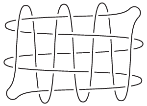
To prove this theorem, we show that the Hempel distance of the 4-bridge position is greater than by the method developed by the second author ([22]). This guarantees that the 4-bridge position is locally minimal (see Lemma 2.1).
On the other hand, Zupan showed that locally minimal, but not globally minimal Morse positions exist even if the knot is trivial.
Theorem 1.6 ([26]).
There exists a locally minimal Morse position of the trivial knot which is not globally minimal.
We remark that this answers Scharlemann’s question [17, Question 3.5]. By using this example, Zupan showed that there exist infinitely many locally minimal, but not globally minimal Morse positions for any knot.
2. Proof of the main theorem
Note that Figure 3 displays a -bridge position of after a -rotation of , and so the -bridge position is not globally minimal. To prove that the -bridge position is locally minimal, we apply the following:
Lemma 2.1.
An -bridge position is locally minimal if it has Hempel distance greater than .
Theorem 2.2 ([22]).
An -bridge position has Hempel distance greater than if a bridge diagram of it satisfies the well-mixed condition.
Here is an integer greater than . The notions of Hempel distance, bridge diagram and well-mixed condition are described in the following subsections.
2.1. Hempel distance
Suppose that is an -bridge position of a knot and is a bridge sphere of . Let be the -balls divided by , and be the arcs for each .
Consider a properly embedded disk in . We call an essential disk of if is disjoint from and is essential in the -punctured sphere . Here, a simple closed curve on a surface is said to be essential if it neither bounds a disk nor is peripheral in the surface. The essential simple closed curves on form a -complex , called the curve graph of . The vertices of are the isotopy classes of essential simple closed curves on , and a pair of vertices spans an edge of if the corresponding isotopy classes can be realized as disjoint curves. The Hempel distance of is defined as
where is the minimal distance between and measured in with the path metric.
Assume that has Hempel distance . By the definition, there exist essential disks of , , respectively, such that , which requires that is split. Since the circle is connected, the Hempel distance is at least . The Hempel distance is if there exist essential disks of , respectively, such that . We can find such disks for a not locally minimal bridge position as follows:
Proof of Lemma 2.1.
Assume that the -bridge position is not locally minimal. By definition, there exist a strict upper disk and a strict lower disk for such that consists of a single point of . Note that is arcs each of which has a single local minimum. We can choose strict lower disks for such that are pairwise disjoint. Let denote a closed regular neighborhood of in . By replacing subdisks of with subdisks of , we can arrange that are disjoint from except for the two points of . Since we assumed , one of the strict lower disks, denoted by , is disjoint from . The boundary of a regular neighborhood in of each intersects in an essential disk of . They guarantee that the Hempel distance is . ∎
2.2. Bridge diagram
We continue with the above notation. There are pairwise disjoint strict upper (resp. lower) disks (resp. , ) for . The knot diagram of obtained by projecting into along these disks is called a bridge diagram of . In the terminology of [5], are the overpasses and the underpasses of .
Now let us describe how we can obtain a bridge diagram of the -bridge position . Isotope as in Figure 8, and start with a bridge sphere . There are canonical strict upper disks and . Figure 8 illustrates a view of the arcs and on from side. Shifting the bridge sphere to , the arcs can be seen as in Figure 8. Shifting further to and to , the arcs are as in Figure 8 and 8, respectively. By continuing this process, the arcs are as in Figure 9 when is at . The picture grows more and more complicated as goes down. We include huge pictures in the back of this paper. Figure 10 illustrates the arcs when is at , and finally Figure 11 when has arrived at . Then we can find canonical strict lower disks and obtain a bridge diagram of .


2.3. Well-mixed condition
Suppose again that is an -bridge position of a knot with and is a bridge sphere of . Let be the -balls divided by , and be the arcs for each . Let and be strict upper and lower disks for determining a bridge diagram of .
Let be a loop on containing the arcs such that the arcs are located in in that order. We can assume that have been isotoped so that the arcs have minimal intersection with . For the bridge diagram of Figure 11, it is natural to choose to be the one which is seen as a horizontal line. Let be the hemi-spheres divided by and let () be the component of which lies between and . (Here the indices are considered modulo .) Let be the collection of components of separating from in for a distinct pair and . For example, Figure 12 roughly displays for the bridge diagram of Figure 11. Note that consists of parallel arcs in .

Definition 2.3.
- (1)
A bridge diagram satisfies the -well-mixed condition if in , a subarc of is adjacent to a subarc of for every distinct pair .
- (2)
A bridge diagram satisfies the well-mixed condition if it satisfies the -well-mixed condition for every combination of a distinct pair and .
By making Figure 12 detailed, one can check the -well-mixed condition for the bridge diagram of Figure 11. One can also check the -well-mixed condition for all the other to complete the well-mixed condition. By Theorem 2.2, the Hempel distance of is greater than . By Lemma 2.1, we conclude the proof of Theorem 1.5.
We would like to remark that the Hempel distance of is exactly . Notice that the boundary of a regular neighborhood in of the closure of is a simple closed curve disjoint from both and . Note that the boundary of a regular neighborhood in of each intersects in an essential disk of . They guarantee that the Hempel distance is at most .
3. Related results and further directions
3.1. The knot of our example
Figure 3 shows that the bridge number of is at most . Since any locally minimal bridge position of any 2-bridge knot is globally minimal ([13], [18]), the bridge number of is equal to . Since has a -bridge position with the Hempel distance , it is a prime knot by the following:
Theorem 3.1.
A bridge position of a composite knot has Hempel distance .
Proof.
Let be an -bridge position of a composite knot and be a bridge sphere of . Let be the -balls divided by , and be the arcs for each . By the arguments in [19], [20], it follows that any decomposing sphere for can be isotoped so that it intersects in a single loop. Then, in the opposite sides of the decomposing sphere, there are two essential disks of respectively such that . This shows that the Hempel distance is . ∎
Furthermore, is hyperbolic since any locally minimal bridge position of any torus knot is globally minimal ([15]). Thus, is a hyperbolic 3-bridge knot which admits a -bridge position with the Hempel distance 2.
We expect that not only may be an example for Theorem 1.5 but also many -bridge positions of knots with the same projection image as that of Figure 3. However only finitely many knots have the same projection image, and we would like to ask the following problem.
Problem 3.2.
For an integer , can we generate infinitely many -bridge positions which are locally minimal, but not globally minimal?
We further expect that for some integers , we can find a locally minimal -bridge position of an -bridge knot which has a similar projection image as that of Figure 3. However it seems difficult to find more than two locally minimal bridge positions of such a knot, and we would like to ask the following problem.
Problem 3.3.
Does any knot have infinitely many locally minimal bridge positions?
It should be remarked that there exist only finitely many bridge positions of given bridge numbers for a hyperbolic knot ([4]). In particular, there are finitely many globally minimal bridge positions of a hyperbolic knot. It should be also remarked that multiple bridge surfaces restrict Hempel distances ([24]).
3.2. Essential surfaces
Composite knots are a simple example of knots with essential surfaces properly embedded in the exteriors of their representatives. Theorem 3.1 suggests that essential surfaces restrict Hempel distances. Bachman–Schleimer showed it in general.
Theorem 3.4 ([3]).
Let be an orientable essential surface properly embedded in the exterior of a bridge position of a knot. Then the Hempel distance of is bounded above by twice the genus of plus .
By Theorem 3.4, if a knot exterior contains an essential annulus or an essential torus, then the Hempel distance of a bridge position is at most 2. Therefore, if there exists a bridge position of a knot with the Hempel distance at least 3, then the knot is hyperbolic. The properties of our knot can be compared with it.
A knot without an essential surface with meridional boundary in the exterior of its representative is called a meridionally small knot. For example, the trivial knot, 2-bridge knots and torus knots are known to be meridionally small. As we mentioned in Section 1, these knots also have the nice property that any nonminimal bridge position is stabilized. We say that a knot is destabilizable if it has this property. Zupan showed that any cabled knot of a meridionally small knot is also meridionally small, and that if is destabilizable, then is also destabilizable ([25]). Then, the following problem is naturally proposed.
Problem 3.5.
Is there a relation between meridionally small knots and destabilizable knots?
We remark that a bridge position of a meridionally small knot is locally minimal if and only if the Hempel distance is greater than by Lemma 2.1 and the following fundamental result:
Theorem 3.6 ([9], [23]).
If a bridge position of a knot has Hempel distance , then either it is stabilized or the knot exterior contains an essential surface with meridional boundary.
On the other hand, it is not always true that if the knot exterior contains an essential surface with meridional boundary, then a bridge position has Hempel distance . For example, [10, Example 5.1] shows that a -bridge position of has Hempel distance greater than , but the knot exterior contains an essential surface with meridional boundary.
3.3. Distance between bridge positions
Theorem 1.1 allows us to define a distance between two bridge positions of a knot, which we call the Birman distance. That is to say, the Birman distance between two bridge positions is the minimum number of Type I moves and the inverse operations relating the bridge positions up to isotopy. For example, the Birman distance between an -bridge position and an -bridge position of the trivial knot is always by Theorem 1.3. The Birman distance between and the -bridge position of is at least since is locally minimal. In fact, we can see that it is at most by observing the -rotation of .
Johnson–Tomova gave an upper bound for the Birman distance between two bridge positions with high Hempel distance which are obtained from each other by flipping, namely the rotation of exchanging the poles.
Theorem 3.7 ([11]).
For an integer , if an -bridge position of a prime knot has Hempel distance at least , then the Birman distance between and the flipped bridge position of is .
They also gave the following, which holds even if we consider bridge positions modulo flipping.
Theorem 3.8 ([11]).
For an integer , there exists a composite knot with a -bridge position and a -bridge position such that the Birman distance is at least .
We remark that the -bridge position is not locally minimal, and hence it does not answer Problem 1.4. It turns out that there are two -bridge positions such that the Birman distance is at least . The following are major problems.
Problem 3.9.
Determine or estimate the Birman distance in terms of some invariants of the bridge positions.
Problem 3.10.
For a given , does there exist a universal upper bound for the Birman distance between locally minimal bridge positions of every -bridge knot?
Acknowledgements. The authors are grateful to Joel Hass for suggesting the construction of the bridge position . They would also like to thank Alexander Zupan for valuable comments.
References
- [1] J. W. Alexander and G. B. Briggs, On types of knotted curves, Ann. of Math. (2) 28 (1926/27), no. 1-4, 562–586.
- [2] J. S. Birman, On the stable equivalence of plat representations of knots and links, Canad. J. Math. 28 (1976), no. 2, 264–290.
- [3] D. Bachman and S. Schleimer, Distance and bridge position, Pacific J. Math. 219 (2005), no. 2, 221–235.
- [4] A. Coward, Algorithmically detecting the bridge number of hyperbolic knots, arXiv:0710.1262.
- [5] R. H. Crowell and R. H. Fox, Introduction to knot theory, Reprint of the 1963 original, Graduate Texts in Mathematics, 57, Springer-Verlag, New York-Heidelberg, 1977.
- [6] D. Gabai, Foliations and the topology of 3-manifolds. III, J. Differential Geom. 26 (1987), no. 3, 479–536.
- [7] C. Hayashi, Stable equivalence of Heegaard splittings of -submanifolds in -manifolds, Kobe J. Math. 15 (1998), no. 2, 147–156.
- [8] C. Hayashi and K. Shimokawa, Heegaard splittings of the trivial knot, J. Knot Theory Ramifications 7 (1998), no. 8, 1073–1085.
- [9] C. Hayashi and K. Shimokawa, Thin position of a pair (3-manifold, 1-submanifold), Pacific J. Math. 197 (2001), no. 2, 301–324.
- [10] D. J. Heath and T. Kobayashi, Essential tangle decomposition from thin position of a link, Pacific J. Math. 179 (1997), no. 1, 101–117.
- [11] J. Johnson and M. Tomova, Flipping bridge surfaces and bounds on the stable bridge number, Algebr. Geom. Topol. 11 (2011), no. 4, 1987–2005.
- [12] J.-P. Otal, Présentations en ponts du nœud trivial, C. R. Acad. Sci. Paris Sér. I Math. 294 (1982), no. 16, 553–556.
- [13] J.-P. Otal, Presentations en ponts des nœuds rationnels, Low-dimensional topology (Chelwood Gate, 1982), 143–160, London Math. Soc. Lecture Note Ser., 95, Cambridge Univ. Press, Cambridge, 1985.
- [14] M. Ozawa, Bridge position and the representativity of spatial graphs, Topology and its Appl. 159 (2012), no. 4, 936–947.
- [15] M. Ozawa, Non-minimal bridge positions of torus knots are stabilized, Math. Proc. Cambridge Philos. Soc. 151 (2011) 307–317.
- [16] K. Reidemeister, Elementare Begründung der Knotentheorie, Abh. Math. Sem. Univ. Hamburg 5 (1927) 24–32.
- [17] M. Scharlemann, Thin position in the theory of classical knots, Handbook of knot theory, 429–459, Elsevier B. V., Amsterdam, 2005.
- [18] M. Scharlemann and M. Tomova, Uniqueness of bridge surfaces for 2-bridge knots, Math. Proc. Cambridge Philos. Soc. 144 (2008), no. 3, 639–650.
- [19] H. Schubert, Über eine numerische Knoteninvariante, Math. Z. 61 (1954), 245–288.
- [20] J. Schultens, Additivity of bridge numbers of knots, Math. Proc. Cambridge Philos. Soc. 135 (2003), no. 3, 539–544.
- [21] J. Schultens, Width complexes for knots and 3-manifolds, Pacific J. Math. 239 (2009), no. 1, 135–156.
- [22] K. Takao, Bridge decompositions with distances at least two, Hiroshima Math. J. 42 (2012), no. 2, 161–168.
- [23] M. Tomova, Thin position for knots in a 3-manifold, J. Lond. Math. Soc. (2) 80 (2009), no. 1, 85–98.
- [24] M. Tomova, Multiple bridge surfaces restrict knot distance, Algebr. Geom. Topol. 7 (2007), 957–1006.
- [25] A. Zupan, Properties of knots preserved by cabling, Comm. Anal. Geom. 19 (2011), no. 3, 541–562.
- [26] A. Zupan, Unexpected local minima in the width complexes for knots, Algebr. Geom. Topol. 11 (2011), no. 2, 1097–1105.

![[Uncaptioned image]](1203.1119v3/x1.png)
The right part of Figure 10.

![[Uncaptioned image]](1203.1119v3/diagram-7.png)
The part of Figure 11.
![[Uncaptioned image]](1203.1119v3/x2.png)
The part of Figure 11.
![[Uncaptioned image]](1203.1119v3/x3.png)
The part of Figure 11.
![[Uncaptioned image]](1203.1119v3/x4.png)
The part of Figure 11.
![[Uncaptioned image]](1203.1119v3/x5.png)
The part of Figure 11.
![[Uncaptioned image]](1203.1119v3/x6.png)
The part of Figure 11.
![[Uncaptioned image]](1203.1119v3/x7.png)
The part of Figure 11.
![[Uncaptioned image]](1203.1119v3/x8.png)
The part of Figure 11.
![[Uncaptioned image]](1203.1119v3/x9.png)
The part of Figure 11.
![[Uncaptioned image]](1203.1119v3/x10.png)
The part of Figure 11.
![[Uncaptioned image]](1203.1119v3/x11.png)
The part of Figure 11.
![[Uncaptioned image]](1203.1119v3/x12.png)
The part of Figure 11.
![[Uncaptioned image]](1203.1119v3/x13.png)
The part of Figure 11.
![[Uncaptioned image]](1203.1119v3/x14.png)
The part of Figure 11.