Modeling active electrolocation in weakly electric fishThanks: This work was supported by ERC Advanced Grant Project MULTIMOD–267184.
Abstract
In this paper, we provide a mathematical model for the electrolocation in weakly electric fishes. We first investigate the forward complex conductivity problem and derive the approximate boundary conditions on the skin of the fish. Then we provide a dipole approximation for small targets away from the fish. Based on this approximation, we obtain a non-iterative location search algorithm using multi-frequency measurements. We present numerical experiments to illustrate the performance and the stability of the proposed multi-frequency location search algorithm. Finally, in the case of disk- and ellipse-shaped targets, we provide a method to reconstruct separately the conductivity, the permittivity, and the size of the targets from multi-frequency measurements.
AMS subject classifications. 35R30, 35J05, 31B10, 35C20, 78A30
Key words. multi-frequency MUSIC algorithm, weakly electric fish, location search algorithm, approximate boundary conditions
1 Introduction
In the turbid rivers of Africa and South America, some species of fish generate an electric current which is not enough for defense purpose. In 1958, Lissmann and Machin discover that this electric current is in fact used for spatial visualization [32]. Indeed an object in the vicinity of the fish will be detected by measurement of the electric field’s distortion on the skin. Behavioral experiments have shown that the weakly electric fish is able to extract useful information about targets, such as the location [50], the shape [49], and the electric parameters (capacitance and conductivity) [48].
Mathematically speaking, this is an inverse problem for the electric field created by the fish. Indeed, given the current distribution over the skin, the problem is to recover the conductivity distribution in the surrounding space. Due to the ill-posedness of this type of problems, it is very difficult to recover as much information as the fish is able to. Thus, modelling this “electric sense” (called active electrolocation) is likely to give us insights in this regard.
Electrolocation has been quantitatively investigated since Lissmann and Machin, who tried an analytical approach. More precisely, they computed the distortion created by a cylinder placed in the electric field of a dipole [32], and noticed that it is equivalent to the field created by a dipole located inside the cylinder. In 1983, Bacher remarked that this formula cannot explain the phase difference observed when the electric permittivity of the target does not equal the permittivity of the water [13]. This phase shift seems to be an important input for the fish since it is measured by receptors (called Rapid Timing units [37]), and thus will be the central point in this paper. Rasnow in 1996 gathered these two previous results by considering a time-harmonic and spatially uniform background electric field. In the presence of a sphere with center at and radius , conductivity , and permittivity , the uniform background electric field with frequency is modified by adding the following field:
| (1.1) |
where the index refers to the ambient medium.
Numerical approaches have also been driven since the 70’s: in 1975, Heiligenberg proposed a finite differences scheme to calculate the field created by the fish [25]. In 1980, Hoshimiya et al. use finite elements to solve this problem [26]. The geometry of the fish is simplified by an ellipse and is divided into two areas: the thin skin with low conductivity and the interior of the body. Their aim is to optimize conductivity values to approximate as better as possible the experimentally measured field. The result is that the optimal conductivity is non-uniform, being higher in the tail region. Improvements of these models since then can be found in [12, 33, 35, 39] and references therein. However, the most promising technique is the use of the boundary element method performed by Assad in the 90’s in his PhD thesis [10]. Indeed, the important feature is the electric potential on the skin (because it is the input for the fish), so a boundary element method (BEM) approach allows us to concentrate the equations on it. Moreover, the computation speed is enhanced because the number of nodes is dramatically reduced. The equation considered is here on the exterior of the body with Robin boundary conditions on the skin [51]:
| (1.2) |
where is the potential inside the body and ( being the skin thickness and (resp. ) the skin (resp. water) conductivity) is the effective skin thickness.
Let us mention that there are other kinds of simulations, based on a more empirical approach, determining an equivalent electric circuit [18, 19] or an equivalent multipole [22].
The aim of this paper is to derive a rigorous model for the electrolocation of an object around the fish. Two problems arise: the direct problem, i.e., the equations involved and their boundary conditions, and the reconstruction itself. For the direct complex conductivity problem, we show using layer potential techniques the validity of (1.2). We also generalize formula (1.1) to the case of a non-uniform background electric field, taking into account the distortion induced by the body of the fish, and with any shape of the target. For the inverse problem, little is known in the complex conductivity case [15]. Here, we take advantage of the smallness of the targets to use the framework of small volume asymptotic expansions for target location and characterization [6, 7]. However, since the electric current is generated by only one emitter at the tail of the fish (the electric organ) and measured by many receptors on the skin, standard non-iterative algorithms such as MUSIC (standing for MUltiple Signal Classification) cannot be applied for location search. In standard MUSIC, the data (called multistatic response matrix) form a matrix and its singular value decomposition leads to an efficient imaging function by projecting the Green function of the medium onto the significant image space [2, 4, 8, 17, 21, 23, 30]. Here, roughly speaking, one has only a column of the response matrix. However, using the fact that the electric current produced by the electric organ is periodically time dependent with a known fundamental frequency, we extend MUSIC approach to multi-frequency measurements by constructing an efficient and robust multi-frequency MUSIC imaging function. We perform numerical simulations in order to validate both the direct model and the multi-frequency MUSIC algorithm. We also illustrate the robustness with respect to measurement noise and the sensitivity with respect to the number of frequencies, the number of sensors, and the distance to the target of the location search algorithm. Finally, in the case of disk- and ellipse-shaped targets, we provide a method to reconstruct separately the conductivity, the permittivity, and the size of the targets from multi-frequency measurements. We mention that this is possible only because of multi-frequency measurements which yield polarization tensors with complex conductivities. It is well-known that polarization tensors for real conductivities cannot separate the size from material properties of the target [7]. We also mention that the use of different values for the frequencies is more crucial for the material and size reconstruction procedure than for the location step. In fact, in the presence of measurement noise, location with realizations with one frequency is comparable to the one with different frequency values.
The paper is organized as follows. In section 2, the model is set up and the equations governing the electric field are rigorously derived. Using layer potential techniques, the boundary condition (1.2) is recovered. In section 3, a small target is located using multi-frequency measurements. For this purpose, a dipolar approximation is derived before the analysis of the response matrix. Finally, numerical simulations are performed in section 4; due to the presence of a hyper-singular operator, a particular attention is paid to the numerical scheme. Reconstructions of the electromagnetic parameters and the size of disk- and ellipse-shaped targets are also provided.
2 The forward problem
The aim of this section is to formulate the forward problem. After the setup of the problem in subsection 2.1, the boundary conditions are announced in subsection 2.1 before being derived in subsection 2.2.2. Existence, uniqueness and a useful representation lemma for this derivation are proved in subsection 2.2.1.
2.1 Non-dimensionalization and problem formulation
In this subsection, we derive the equations governing the electric field. A formal explanation of the electroquasistatic (or EQS) formulation is given, and the setup of the problem is then non-dimensionalized.
Partial differential equations of the problem
The electroquasistatic (or EQS) formulation is a low-frequency limit for the Maxwell system in three dimensions. In the frequency domain, this latter is given by
| (2.1) |
where is the electric field, is the magnetic induction field, and are the free charges and currents, is the frequency, is the magnetic permeability, and is the electric permittivity. Moreover, in a medium of conductivity the Ohm’s law connects the electric field to the induced current density () so the current density can be decomposed as:
where is a source of current (in our model, it comes from the electric organ). Then, taking the divergence of the last line in (2.1), we have:
| (2.2) |
The EQS approximation consists in considering the electric field as irrotational because the magnetic field variation is negligible. A sufficient condition for that is given by [46]:
| (2.3) |
where is the maximal length of the problem and the minimal wavelength. Here, we can take m because the range of electrolocation does not exceed two body lengths [37]. In the water, the minimal wavelength is given by
where , and is the maximal frequency emitted by the fish, which is of the order of kHz. Thus, the fraction in (2.3) is of order , so the EQS approximation is very well suited for our situation.
Going back to the equation of the electric field (2.2), we can now use the fact that is irrotational to state that it is derived from a potential scalar field . This finally leads us to the following equation:
| (2.4) |
To conclude, taking into account the slow variation of the electric field leads us to consider a complex conductivity instead of a real valued one. However, for the rest of this section, the imaginary part of this conductivity will be neglected; indeed measurements on a Gnathonemus petersii showed that the permittivity of the skin, the body, and the water are very small compared to their respective conductivity [19, 40]. Thus, this EQS approximation will be used only in the presence of a target: it will be detected by the phase shift induced by its complex conductivity.
Non-dimensionalization
We wish to perform an asymptotic analysis of the equations. The first step consists in the identification of the different scales of the model problem. The electric potential , the variables and , and the parameters and can be written as follows:
where is the voltage produced by an electric organ discharge (EOD), is the length of the fish, is the fundamental frequency of the EOD, is the conductivity of the surrounding water and is the current intensity inside the electric organ. Moreover, anticipating the next subsection, the conductivity of the body and the skin play an important role in the shape of the electric field. Thus, in the list of parameters we add the conductivity of the body , the thickness of the skin and its surface conductivity . The orders of magnitude of these parameters are found in Table 2.1.
| Quantity | Order of magnitude | Reference |
|---|---|---|
| mV | [11, 44] | |
| cm | [37] | |
| kHz | [37] | |
| Scm-1 | [34] | |
| mA | [14] | |
| Sm-1 | [40] | |
| Scm-2 | [19] | |
| m | [52] |
These quantities involve fundamental units of the SI system, so according to the Buckingham-Pi theorem, we need nondimensional quantities. The first one can be found by rewriting the equation (2.4) in terms of the nondimensional quantities ():
| (2.5) |
The multiplicative term in the right-hand side of the previous equation is not important as the equation is linear. The three other nondimensional quantities come from the parameters of the skin and the body of the fish:
In other words, in nondimensional units, (resp. ) is the body (resp. skin) conductivity and is the skin thickness.
To conclude, omitting the prime symbol for the sake of clarity and denoting by the source term in equation (2.5), the governing PDE is the following
| (2.6) |
where is piecewise constant, being equal to in the water, inside the body of the fish and in the skin. These domains are going to be made precise in the next subsection.
For the sake of simplicity, from now on, we only consider the model equations in two dimensions.
2.2 Boundary conditions
In this subsection, we derive the appropriate boundary conditions associated with the presence of a very thin and very resistive skin. Robin boundary conditions will be found after an asymptotic analysis of the layer potentials involved.
The setup is as follows: the body occupies a fixed smooth open set and the skin with constant thickness is described as:
where is the outward normal unit vector. Let us also denote by the effective thickness defined by Assad [51]; in our variables it is given by
The source of the electric field is a sum of Dirac functions:
where, for , and satisfies the charge neutrality condition
| (2.7) |
Although condition (2.7) is the physical condition in our model, we will show how to modify the derivations and the results of the paper in the general case. An illustration is given in Figure 2.1.
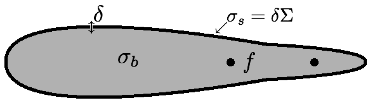
Our main purpose here is to investigate the behavior of the solution of (2.6) with
| (2.8) |
where and , in the following asymptotic regime:
In order to make this dependence clear, let us denote such a solution by . Adding a far field condition (essential for uniqueness, see subsection 2.2.1), it is the solution of
| (2.9) |
where and is given by (2.8). Note that if assumption (2.7) does not hold, then the far field condition should be replaced with
| (2.10) |
where the parameters and are given by
| (2.11) |
The far field condition (2.10) will be explained later. We will compute the first-order asymptotic and see that it is the solution of the following system:
| (2.12) |
Note that in the limiting model (2.12), the role of is to fix the potential on . On the other hand, if assumption (2.7) does not hold, then the boundary condition on should be replaced with
To be more precise, we will prove the following theorem:
Theorem 1.
In a first part, we will analyze equation (2.9) and show that there exists a unique solution that can be represented as the sum of a harmonic function and two single-layer potentials. In a second part, we will perform asymptotic analysis of these layer potentials in order to show that the limiting function is solution of (2.12). This latter part is to adapt the work done by Zribi in his thesis [53] and by Zribi and Khelifi in [29].
2.2.1 Existence, uniqueness, and representation of the electric potential
In this part, we will first prove the uniqueness of the solutions of (2.9) and then we will derive a representation formula, which will give us the existence of the solution. For the moment, and are fixed, but we suppose that:
| (2.14) |
Uniqueness
The uniqueness comes from the second line of (2.9) [7]. Indeed, let , where and are two solutions of (2.9) and let us show that . From (2.14) we get, for sufficiently large (so that the ball with center and radius encompasses ):
Here we have used the fact that , which holds as a consequence of the far field condition. A unique continuation argument shows that in and thus is constant. Then, using the fact that as , we have .
Existence and representation
The existence is given by a representation formula decomposing the solution into a source part and a refraction part. This refraction part implies layer potentials on the boundaries of the body and the skin. Let us define them explicitly and give some well-known results. First, let us define the following boundaries:
In the following, the index stands for the subscript or . The single- and double-layer potentials on are operators that map any to and , respectively, where
where is the Green function for the Laplacian in :
| (2.15) |
For , the functions and are harmonic functions in ; their singularities hold on . To describe these singularities, we define, for a function defined in and :
Across the boundary , the following trace relations hold [7]:
| (2.16) | ||||
Here, the operator and its -adjoint are given by
where stands for the Cauchy principal value. From (2.16) it follows that the following jump formulas hold:
Theorem 2.
Suppose that has Lipschitz regularity. Then the operator is invertible on if , and for , is invertible on .
With these essentials tools, we can now prove the following decomposition formula in the same spirit as in [27]:
Lemma 1.
Proof.
The system (2.9) is equivalent to the following transmission problem [1]:
The existence of a solution to (2.19) comes from the fact that and Theorem 2. On the other hand, the functions and are harmonic in , and according to the definition of , we have in . In and , all these functions are harmonic so we have . The trace relations on and are then given by the singularities (2.16) of and (see [7]) since is smooth away from the points . Finally, all these functions are controlled by when . In this way, the existence of a solution to (2.9) is proved.
To prove the uniqueness of the decomposition, let us take and such that
Then, is harmonic in , which gives by the jump formula . Finally, applying once more the jump formula, we have . ∎
We now check the far field condition stated in (2.10). Recall that . From
by taking the average of the two equations in (2.19) on and , respectively, we find that
and therefore, from the representation formula (2.17) it follows that
Note that in the limit and , the far field condition above and (2.11) yield , and therefore,
| (2.20) |
Lemma 2.
In the general case, (2.22) should be replaced with
Note that since , the far field condition (2.20) is satisfied in the general case.
The proof of this lemma involves exactly the same arguments as in the previous one: jump formulas applied to the operators.
2.2.2 Asymptotic expansion of the electric potential for highly resistive skin and highly conductive body
In this part, we will use the decomposition formula for and compute asymptotic expansions of the refraction part. The limiting solution will then be . This latter is well defined if the limits and are independent, so we must seek the two following limits:
and show that they are the same. Zribi [53, chapter 3] studied the case when remains fixed, with non-uniform thickness of the skin ; the limit is the solution of the system:
| (2.23) |
Here, we will follow the same outline for the proof: first we will remind the asymptotic expansions of the operators involved in (2.19), and then we will match the asymptotic expansions for and .
Asymptotic expansions of the operators
In the decomposition formula (2.17), is independent of and ; we just have to analyze the dependence of and . Remark that from (2.19)
- •
the dependence on is carried only by since and depend only on the shape of ;
- •
the dependence on is carried by , , and for .
In this subsection, we will focus on the asymptotic expansions of the operators (the limits of and are obvious). They have been performed in [9, 53]; in order to apply this proof, we first need some assumptions.
Suppose is defined in the following way:
where is a diffeomorphism of the unit sphere for some . Moreover, we suppose that the function defined by
is such that for all . Thus, is a arclength counterclockwise parametrization of . Then the outward unit normal to , at , is given by
where is the rotation by . The tangential vector at is defined by
and . The curvature at is defined by
Let be the diffeomorphism from onto given by
| (2.24) |
With these assumptions, the following regularity result holds [31]:
Theorem 3.
Let . Let, for a Lipschitz function ,
Introduce the set of admissible diffeomorphisms of the unit sphere:
Then, for any integer , the operators and defined on (, respectively) to by
are jointly analytic with respect to their variables and .
Moreover, we have explicit formulas for the derivatives with respect to the variable [31].
Proposition 1.
Let and for some . Then, we have the following asymptotic expansions for :
| (2.25) | ||||
where , being defined by (2.24), and
| (2.26) | ||||
where is the tangential derivative in the direction of .
Note that, according to Theorem 3, the constants in the terms depend on .
Moreover, since the thickness of is uniform, we have , and a Taylor expansion of gives, for :
| (2.27) |
where denotes the Hessian of .
Asymptotic expansions on the layers
In order to prove Theorem 1, we will first show the convergence on the layers (see next lemma). Then, in the next subsection, we will extend the domain of validity by application of the maximum principle.
The following lemma holds.
Lemma 3.
Proof.
Only the first limit will be shown, the second one being very similar. For this purpose, we must show that the limits and are independent, i.e., they commute. First, let us compute the limit of when , and then the limit (which will be much easier). Then, we will invert this process.
This first limit is the main problem in [53, chapter 3], except that, in that study, and the thickness of is non-uniform. According to theorem 3, the formulas in [31], and by composition with the regular diffeomorphism from to , we have
where . Hence, with the help of the decomposition formula (2.17), we have the following asymptotic expansion uniformly on :
| (2.29) |
We now look for expansions of the functions and when that will be re-injected in this equation. Using Proposition 1 and (2.19), these functions are solutions of the following system:
| (2.30) |
Let us define the formal asymptotic expansions:
Aiming to have the -order term in the expansion (2.29), here we seek for the terms of order and . By substitution into (2.30) and identification of the leading-order terms in the first line, we get:
so that, by Theorem 2, we have:
| (2.31) |
Let us now look at the -order terms; summing the two lines, we get:
which gives, with the help of (2.26) and (2.31),
| (2.32) |
This quantity is what we need in (2.29); thus, only remains to be found. This can be done by identification of the -order terms in the first line of (2.30) and using the definitions of and given by (2.26):
| (2.33) |
Finally, the expansion (2.29) yields:
| (2.34) |
This leading-order term (denoted ) verifies (2.23) according to (2.33) and jump formulas (2.16).
The asymptotic does not add further difficulty. Indeed, let us define the following asymptotic:
By substitution into equation (2.33) and identification of the leading-order terms, we get:
and then the expansion (2.34) becomes:
| (2.35) |
which is (2.21) applied on according to the jump formula of (2.16). Hence, according to lemma 2, the first-order asymptotic of is .
Let us now show that the limits and commute: unlike in the previous subsection, we will first perform the limit and then the limit . Given the fact that
the definition of and in (2.19) will be affected only in the second line. Indeed, with the following expansions:
this second line becomes, at the leading order:
where . With the expansion:
the identifications (2.31), (2.32), and (2.33) respectively become:
| (2.36) |
| (2.37) |
Proof of Theorem 1
With the estimates (2.28) on the layers and , we are now ready to prove the estimate (2.13) on the whole space applying the maximum principle.
For the sets and , it is straightforward: the function is harmonic in these bounded domains, so the maximum is reached on the boundaries [45]. And, since this maximum is dominated by and , we have:
For the exterior domain, we cannot apply directly the maximum principle since this domain is unbounded. However, the conditions at infinity in the systems (2.9) and (2.12) allow us to have a similar control. Indeed, this condition tells us that
| (2.39) |
We take:
and choose such that, for , the right-hand side of (2.39) is bounded by . Then, we have:
Now, only the bounded domain remains, where we can apply the maximum principle. Thus, Theorem 1 is proved.
2.3 Final formulation and notation
In the previous subsections, we have performed a multi-scale analysis of the problem to identify the effective equations with boundary conditions. In order to make things clear, let us summarize the results and simplify the notation.
The electric potential emitted by the fish is the solution of the complex-conductivity equation (2.6) with boundary conditions given by the system (2.12). It is easy to see that in the case of an inhomogeneity outside the body, these boundary conditions will not be changed because the asymptotics are done with the layer potentials of the domains defining the fish.
Hence, we conclude this section by summing up the results: omitting all the subscripts, the electric potential is the solution of the system
| (2.40) |
where is the characteristic function of the target , is the conductivity inside , is the frequency, and and are positive constants. Here, we have assumed that . In the case where it is not, we should replace the boundary condition on with . From now on, we restrict ourselves to the case . Note that taking two points and close enough and yields an approximation of a dipole at of moment and direction orthogonal to .
3 Detection algorithm for multi-frequency measurements
In this section, we develop an algorithm to recover (from a single measurement) the location of a small object located far away from the fish. This algorithm is based on multi-frequency measurements, as it is explained in subsection 3.1. In subsection 3.2, asymptotic expansions will be carried out for the electric field in the presence of a small and distant target. Finally, the algorithm will be explained in detail in subsection 3.3.
3.1 Multi-frequency measurements
Let us suppose that the electric current produced by the electric organ, (i.e., the source term in equation (2.40)) is periodically time-dependent with separation of variables, that is
where is a sum of Dirac functions and is periodic with fundamental frequency . Hence, we set
| (3.1) |
where is the upper bound that ensures the low-frequency regime. According to the previous section, the electric potential is then given by
| (3.2) |
where , for , is solution of the following system
| (3.3) |
3.2 A dipolar expansion in the presence of a target
In this subsection, we derive useful formulas in order to simplify the data. For the sake of simplicity, and for numerical reasons that will be given in section 4, only one target will be considered.
The electroreceptors of the fish measure the electric current at the surface of the skin [37]. Hence, from a single measurement, we can construct the Space-Frequency Response (SFR) matrix , whose terms are given by
where are points on the boundary and is the static background solution, i.e., the electric potential without any target which does not depend on . It is the solution of (3.3) with a constant conductivity equal to outside the body .
The first formula, given in Proposition 2, is often called a dipolar expansion; indeed, in the presence of a small inhomogeneity, the perturbation of the electric potential looks like the electric potential of a dipole [6, 20]. More precisely, using exactly the same arguments as in [6, Chapter 4] and in [5] we have the following result.
Proposition 2.
If with , and is an open set, then we have
| (3.4) |
where denotes the transpose, is the (complex) conductivity of the target at the frequency , is the first-order polarization tensor associated to with conductivity [7]:
and is the Green function associated to Robin boundary conditions, which is defined for by
| (3.5) |
Proof.
Let
We have
and on the other hand,
From the transmission condition
it follows that
| (3.6) |
Since
for some constant , provided that , a scaling of the integral in (3.6) together with a Taylor expansion of gives the desired asymptotic expansion. Note that the approximation in (3.4) is uniform in and [7]. ∎
Now, we will carry on a second formula in order to simplify this equation. Indeed, the Green function associated to Robin boundary conditions is tedious to compute. Instead, we will post-process the data thanks to the following lemma which generalizes Lemma 2.15 in [6].
Lemma 4.
Let denote the Green function in the free space defined by (2.15). For and , let and . Then
Proof.
Hence, after a calculation of on , we will apply the post-processing operator given in Lemma 4. The modified matrix will still be denoted .
To conclude, the location of the target is going to be recovered from the knowledge of the following data
| (3.7) |
which is approximately equal to
| (3.8) |
when the characteristic size of the target is small. It is worth mentioning that the polarization tensor is symmetric (but not Hermitian) [7].
3.3 A location search algorithm
Scholz described in [42] a way to recover the location of a target from multi-frequency measurements. The paper focuses on an application in electrical impedance tomography (EIT) for breast cancer detection; the algorithm was called “Space-Frequency MUSIC”. Indeed, it is based on the so-called MUSIC algorithm, which is a standard tool in signal theory for the identification of several signals with an additive noise [41, 16]. It has then been applied to identify small conductivity inhomogeneities in [3, 8, 17]. In this section, we apply a similar approach for our model.
As we can see in formula (3.8), the rows of the SFR matrix are - to leading-order - linear combinations of the derivatives of . Moreover, one has to distinguish whether the target is a disk or not. Indeed, in dimension and in the case of an ellipse whose semi-axes are on the -axis and of length and , the polarization tensor , for , takes the form [36]
Hence, the polarization tensor is proportional to the identity
matrix if and only if , i.e., is a disk; this
result remains true in dimension
[7]. This changes dramatically the range
of : if is a disk, the response matrix
has rank and if it is an ellipse, it has rank .
For the sake of simplicity, let us suppose that is the unit disk.
The identification process will be based on the following fact
Lemma 5.
The following map
is one-to-one.
Proof.
Suppose that and are points on such that . Let us define the two following functions
Thus, these two functions both solve the following boundary value problem
Hence, by the uniqueness of the solution for this problem, we have
Relying on the singularity of at the point , this is only possible if .
∎
However, we do not have access to the complete function (because there is only a finite number of electroreceptors on the body), and the formula for is only an approximation, based on (3.8). The location of the target will then be approximated as follows. In the following we suppose for the sake of simplicity that are equi-distributed on .
Proposition 3 (Space-Frequency MUSIC).
Define the vector
| (3.9) |
and its normalized version . Then, in the limit and , the following imaging functional will have a large peak at :
| (3.10) |
where is the orthogonal projection onto the first singular vector of the SFR matrix .
Proof.
First of all, let us rewrite (just for this proof) the projection and the illumination vector , in order to take into account the dependence with respect to . When goes to infinity, quadrature formulas show us that
Here, is the projection onto the first singular vector of the operator , acting on the space of functions that have the form (3.1)
where is given by (3.2) and is the background solution (i.e., the solution of (3.3) with ).
In the limit , is approximated by the operator , which is obviously of rank one. By theory of perturbation [28], one has therefore
where is the projector onto the first significant singular vector of . Then, from Lemma 5, this functional is zero if and only if .
∎
Moreover, in order to have a general algorithm which is robust with respect to the background solution, we will plot the following imaging functional:
| (3.11) |
where is defined in Proposition 3 and is the normalization of the following vector
Numerical results will be given in section 4.
Let us highlight the fact that in the case of a general shape , we do not know theoretically what happens. Indeed, when is real, is equivalent to the polarization tensor of an ellipse [17], but this is not true when because the proof relies on the spectral theorem. Here, we still have symmetry [7], but it is not sure if is diagonalizable or not. However, we will see in the numerical subsection 4 that the algorithm works with shapes other than ellipses and disks.
4 Numerical simulations
In this section, numerical results are presented in order to illustrate the multi-frequency location search algorithm introduced in the previous section. In the first subsection, we explain the method used to compute the electric field; this will be the input of our location search algorithm that will be performed in the second subsection.
4.1 Direct problem
This section is devoted to the computation of the electric field around the fish.
4.1.1 The case without target
The electric field generated by the fish is the function treated in section 2. Let us recall that it is the solution of the following system:
| (4.1) |
Numerical simulations will be done using a boundary element method (BEM). Indeed, we need accuracy on the skin of the fish, and the jumps at the boundaries are too difficult to handle with a finite element method. Moreover, it reduces the number of discretization points, resulting in a much faster algorithm.
This BEM simulation relies on the representation formula for in terms of the layer potentials. From Lemma 2, we have where in the whole space, and the potentials are solutions of the system:
| (4.2) |
Note that we have changed a little bit the notation, in order to be able to test the case . On smooth domains, the operator is easy to handle because its kernel has integrable singularity, whereas the operator is an hypersingular operator. Thus, one has to perform a integration by parts in order to regularize it: for two smooth functions and , we have (for example from [38, Theorem 1] and [43, Theorem 6.15]):
| (4.3) |
where is the surface rotational, defined in the following way in dimension . First, let us define the vector:
where is an extension of into a neighborhood of , i.e., with the local projection onto . Then is defined by
In our context, this can be made much easier. Recalling the notation of subsection 2.2.2, we have
Thus we have, for ,
Hence, denoting by the curvilinear derivative of on , formula (4.3) becomes
This enables us to derive a BEM formulation of the system (4.2); however one has to perform it with elements instead of simple elements in the case of .
4.1.2 The case with a target
In this subsection, we derive the modification induced on the system (4.2) in the presence of a target of (complex) conductivity . The system (4.1) becomes:
| (4.4) |
Thus, can be written as
The absence of is justified by the continuity across the boundary of . From the jump formulas (2.16), the conditions on the boundaries and given in (4.4) leads us to the following system:
| (4.5) |
where
System (4.5) can be rewritten as follows:
with
The BEM formulation is then also classical, because the only difficulty is due to the hypersingular operator in the upper left term. Hence, we discretize with elements and with elements.
4.1.3 Direct simulations
In this subsection, we present some numerical simulations of the direct problem. We approximate the shape of the fish by an ellipse with semi-axes of lengths and ; the electric organ is a dipole in the -direction of moment , placed at and the impedance is . A ball of infinite conductivity (more precisely, with and ) and radius is located at . Figure 4.1 shows the isopotentials. In Figure 4.1 (b) it can be seen that the isopotentials avoid the target since it is of infinite conductivity.
 |
 |
| (a) | (b) |
4.2 Target location
In this subsection, we show numerical target location results using the imaging function (3.11). With the same parameters used for Figure 4.1 for the fish, but with a small target of electric parameters and , we obtain the imaging functional plotted in Figure 4.2 (a). We use frequencies equidistributed from to . In Figure 4.2 (b) and (c), we have tested other shapes for the target.


Stability estimates with respect to measurement noise
Let us first notice that, in the absence of noise, the number of used frequencies does not change significantly the image. Indeed, we can see in Figure 4.3 that we can recover the location of the target with only one frequency.

Let us now consider the effect of measurement noise on the performance of the location search algorithm. We add to the entries of the matrix defined in (3.8) independent Gaussian random variables of mean and standard deviation
The parameter is the relative strength of the noise, and will be given in . Figure 4.4 shows that increasing the number of frequencies stabilizes the image.


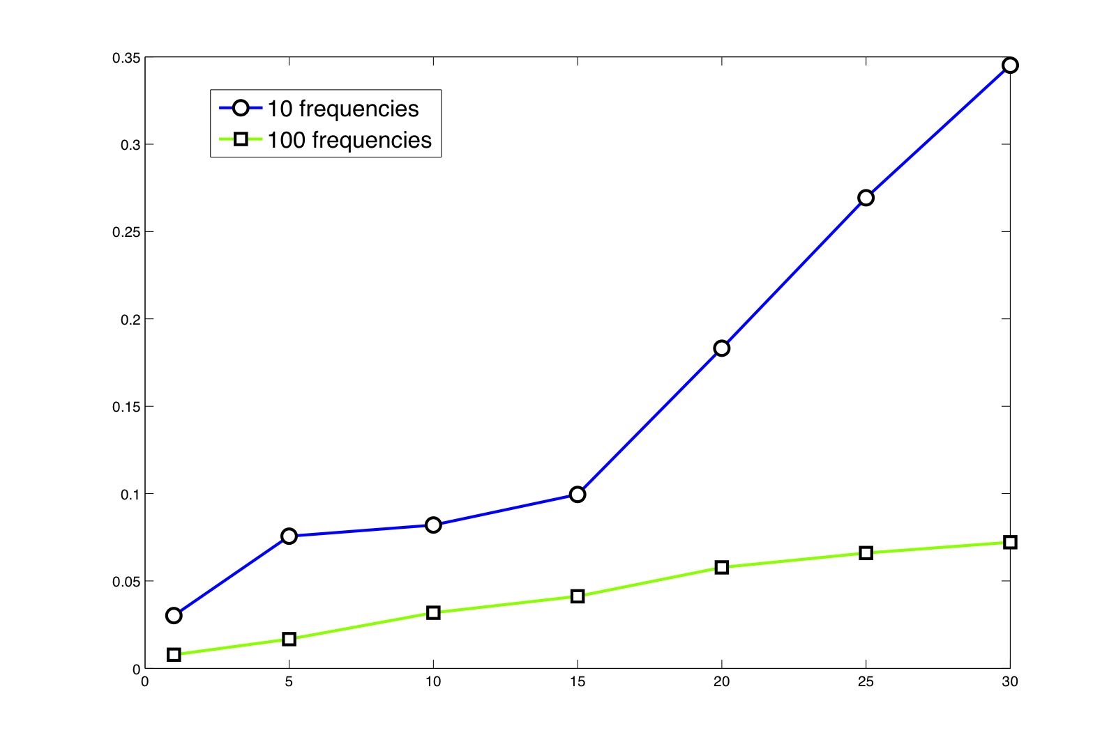
More quantitatively, we have computed the empirical root mean square location error (between the exact location of the target and the maximum of the imaging functional), for trials. Here, the same target as in Figure 4.3 is considered. Results are shown in Figure 4.5.
A natural question is whether taking different values for the frequencies plays a role. In Figure 4.6, we use the data obtained by trials for of noise, sensors, and a single frequency equal to . Figure 4.6 shows that the values of the frequencies do not play a crucial role in the location procedure. In fact, the location result is similar to the one in Figure 4.4. However, from a practical point of view, using simultaneously different frequencies yields a faster robust location procedure than repeating times the data acquisition procedure with the same frequency. In subsection 4.3, we also identify the more fundamental role of the values of the frequencies in the characterization procedure.

The number of sensors is also crucial in the stability of the algorithm. Figure 4.7 compares the root mean square location error with frequencies equidistributed from to for and sensors for different measurement noise levels.

The same type of statistics is possible for the detection as function of the distance between the fish from the target. In Figure 4.8, we have plotted the root mean square location errors, with frequencies equidistributed from to and of noise, for disks with radius placed at for and .

4.3 Target characterization
Once the target is located, one can use (3.8) to estimate the electromagnetic parameters and the size of the target. Assume that the target is a disk of radius , placed at . From (3.8) it follows that can be estimated for from the measurement matrix . Here, with being known. Let be the estimated values of from . To characterize the target and approximate its size, one minimizes the following quadratic misfit functional:
| (4.6) |
over and .
Table 4.1 gives the result of the optimization algorithm for a disk-shaped target with center center and radius . The electromagnetic parameters are . The initial guess is The data is collected for frequencies equidistributed from to . The reconstructed results are accurate.
| 0.05 | 5 | 1 | 0.0506 | 4.9882 | 1.0004 |
|---|---|---|---|---|---|
| 0.05 | 4 | 1 | 0.0506 | 3.9993 | 0.9998 |
| 0.05 | 5 | 2 | 0.0506 | 4.9868 | 2.0017 |
| 0.06 | 5 | 1 | 0.0607 | 4.9878 | 1.0003 |
| 0.04 | 3 | 2 | 0.0404 | 2.9614 | 1.9806 |
When the target is an ellipse, the measurement matrix may not be sufficient to characterize the electromagnetic parameters and the size of the target. At least two different positions of the fish (or equivalently two different locations of the target in the fish frame of reference) are needed in order to generate non-parallel dipole directions at the location of the target and consequently lead to the extraction of the polarization tensor of the ellipse-shaped target . Consider two target locations and in the fish frame of reference. Multi-frequency measurements lead to two SFR matrices, and with and . Define the following linear application from the set of complex symmetric matrices to
For a fixed , we define the data
By a least-squares method, we recover an estimation of the polarization tensor :
Again, once is estimated, a minimization approach yields correct parameter and size values. Since for any , the eigenvectors of the matrix are the ellipse axes, denoting and the estimated complex eigenvalues of , one minimizes the following quadratic misfit functional
over and , in order to reconstruct the semi-axis lengths and and the material parameters and of the ellipse-shaped target .
If is large enough, then semi-analytical formulas to estimate the semi-axis lengths and the material parameters hold. Since
one can estimate and as follows:
| (4.7) |
Table 4.2 gives estimations of and . The target is centered at and the fish moves in the horizontal axis so that . The material parameters of the target are and . The data is collected for frequencies equidistributed from to . The reconstructed results are accurate.
| 0.04 | 0.04 | 0.0390 | 0.0405 |
|---|---|---|---|
| 0.05 | 0.05 | 0.0497 | 0.0516 |
| 0.05 | 0.06 | 0.0586 | 0.0608 |
| 0.03 | 0.06 | 0.0313 | 0.0567 |
| 0.06 | 0.05 | 0.0406 | 0.0487 |
| 0.01 | 0.03 | 0.0108 | 0.0273 |
Moreover, once the geometric parameters and are estimated, it is straightforward to recover and . Introduce
From
one can estimate and as the real and imaginary parts of . However, as shown in Figure 4.9, one can see that the error on the real part is growing with the frequency. Therefore, in order to increase the robustness of the material parameter estimations, one estimate using the lowest frequencies (for example the first three) and using all the frequencies:
| (4.8) |

Table 4.3 gives the material estimations using formula (4.8) for a disk and an ellipse. Once again the results are accurate.
| 2 | 1 | 1.9167 | 1.0661 | |
| disk | 3 | 2 | 2.8481 | 2.0516 |
| 5 | 1 | 5.8884 | 1.4668 | |
| 2 | 1 | 1.7943 | 1.0473 | |
| ellipse | 3 | 2 | 2.7208 | 2.0415 |
| 5 | 1 | 6.0886 | 1.5828 |
5 Conclusion
In this paper, we have proposed a complex conductivity model problem for the quantitative analysis of active electro-location in weakly electric fish. We have rigorously derived the boundary conditions to be used. We have proposed a non-iterative location search algorithm based on multi-frequency measurements. We have presented some numerical results which are promising. We have seen that increasing the number of frequencies (with not necessary different values) improves the stability. In fact, using multi-frequency measurements increases the signal-to-noise ratio. On the other hand, using different frequencies yields a faster robust location algorithm than repeating the data acquisition procedure with the same frequency. We have also proposed a procedure to reconstruct the electromagnetic parameters and the size of disk- and ellipse-shaped targets. This has been possible only because of multi-frequency measurements corresponding here to different frequency values. The use of multi-frequency measurements is fundamental in the characterization procedure. It has been known that polarization tensor for real conductivities cannot separate the size from material properties of the target [7]. For arbitrary-shaped targets, many important questions remain. In particular, it would be interesting to know how much parameter and size information one can extract from its polarization tensors for different complex conductivities. It is also worth mentioning that limiting our asymptotic expansions with respect to the target size to the first-order term (the dipole approximation) does not give us the shape of the target. Hence, in a forthcoming work we will investigate how much information can be acquired in the near field by approaching the fish next to the target and developing the asymptotic expansions with high-order generalized polarization tensors [6]. We will also investigate the stability of the proposed algorithm with respect to random fluctuations in the background permittivity and propose an original cross-correlation technique in order to correct for the effect of random heterogeneities on target location.
References
- [1] G. Allaire. Numerical analysis and optimization. Numerical Mathematics and Scientific Computation. Oxford University Press, Oxford, 2007.
- [2] H. Ammari, J. Garnier, H. Kang, W.K. Park, and K. Sølna. Imaging schemes for perfectly conducting cracks. SIAM J. Appl. Math., 32:894–922, 2010.
- [3] H. Ammari, R. Griesmaier, and M. Hanke. Identification of small inhomogeneities: asymptotic factorization. Math. Comp., 76(259):1425–1448, 2007.
- [4] H. Ammari, E. Iakovleva, and D. Lesselier. A music algorithm for locating small inclusions buried in a half-space from the scattering amplitude at a fixed frequency. SIAM Mult. Scal. Model. Simul., 3:597–628, 2005.
- [5] H. Ammari and H. Kang. High-order terms in the asymptotic expansions of the steady-state voltage potentials in the presence of conductivity inhomogeneities of small diameter. SIAM J. Math. Anal., 34(5):1152–1166, 2003.
- [6] H. Ammari and H. Kang. Reconstruction of small inhomogeneities from boundary measurements. Number 1846. Springer Verlag, 2004.
- [7] H. Ammari and H. Kang. Polarization and moment tensors: with applications to inverse problems and effective medium theory. Springer Verlag, 2007.
- [8] H. Ammari, H. Kang, E. Kim, K. Louati, and M.S. Vogelius. A music-type algorithm for detecting internal corrosion from electrostatic boundary measurements. Numer. Math., 108(4):501–528, 2008.
- [9] H. Ammari, H. Kang, M. Lim, and H. Zribi. Conductivity interface problems. part i: small perturbations of an interface. Trans. Amer. Mathem. Soc., 362(5):2435–2449, 2010.
- [10] C. Assad. Electric field maps and boundary element simulations of electrolocation in weakly electric fish. PhD thesis, California Institute of Technology, 1997.
- [11] C. Assad, B. Rasnow, P.K. Stoddard, and J.M. Bower. The electric organ discharges of the gymnotiform fishes: Ii. eigenmannia. Journal of Comparative Physiology A: Neuroethology, Sensory, Neural, and Behavioral Physiology, 183(4):419–432, 1998.
- [12] D. Babineau, A. Longtin, and J.E. Lewis. Modeling the electric field of weakly electric fish. Journal of experimental biology, 209(18):3636, 2006.
- [13] M. Bacher. A new method for the simulation of electric fields, generated by electric fish, and their distorsions by objects. Biological Cybernetics, 47(1):51–58, 1983.
- [14] C.C. Bell, J. Bradbury, and C.J. Russell. The electric organ of a mormyrid as a current and voltage source. Journal of Comparative Physiology A: Neuroethology, Sensory, Neural, and Behavioral Physiology, 110(1):65–88, 1976.
- [15] E. Beretta and E. Francini. Lipschitz stability for the electrical impedance tomography problem: the complex case. Comm. Partial Differential Equations, 36:1723–1749, 2011.
- [16] L. Borcea, G. Papanicolaou, C. Tsogka, and J. Berryman. Imaging and time reversal in random media. Inverse Problems, 18:1247–1279, 2002.
- [17] M. Brühl, M. Hanke, and M.S. Vogelius. A direct impedance tomography algorithm for locating small inhomogeneities. Numer. Math., 93(4):635–654, 2003.
- [18] R. Budelli and A.A. Caputi. The electric image in weakly electric fish: perception of objects of complex impedance. Journal of Experimental Biology, 203(3):481, 2000.
- [19] A.A. Caputi, R. Budelli, K. Grant, and C.C. Bell. The electric image in weakly electric fish: physical images of resistive objects in gnathonemus petersii. Journal of experimental biology, 201(14):2115, 1998.
- [20] D.J. Cedio-Fengya, S. Moskow, and M.S. Vogelius. Identification of conductivity imperfections of small diameter by boundary measurements. continuous dependence and computational reconstruction. Inverse Problems, 14:553, 1998.
- [21] D.H. Chambers and J.G. Berryman. The linear sampling method and the music algorithm. Inverse Problems, 22:2145–2163, 2006.
- [22] L. Chen, J.L. House, R. Krahe, and M.E. Nelson. Modeling signal and background components of electrosensory scenes. Journal of Comparative Physiology A: Neuroethology, Sensory, Neural, and Behavioral Physiology, 191(4):331–345, 2005.
- [23] M. Cheney. The linear sampling method and the music algorithm. Inverse Problems, 17:591–595, 2001.
- [24] L. Escauriaza, E.B. Fabes, and G. Verchota. On a regularity theorem for weak solutions to transmission problems with internal Lipschitz boundaries. Proc. Amer. Math. Soc., 115(4):1069–1076, 1992.
- [25] W. Heiligenberg. Theoretical and experimental approaches to spatial aspects of electrolocation. Journal of Comparative Physiology A: Neuroethology, Sensory, Neural, and Behavioral Physiology, 103(3):247–272, 1975.
- [26] N. Hoshimiya, K. Shogen, T. Matsuo, and S. Chichibu. Theapteronotus eod field: Waveform and eod field simulation. Journal of Comparative Physiology A: Neuroethology, Sensory, Neural, and Behavioral Physiology, 135(4):283–290, 1980.
- [27] H. Kang and J.K. Seo. The layer potential technique for the inverse conductivity problem. Inverse Problems, 12(3):267–278, 1996.
- [28] T. Kato. Perturbation theory for linear operators. Springer-Verlag, Berlin, second edition, 1976. Grundlehren der Mathematischen Wissenschaften, Band 132.
- [29] A. Khelifi and H. Zribi. Asymptotic expansions for the voltage potentials with two-dimensional and three-dimensional thin interfaces. Math. Meth. Appl. Sci., 34(18):2274–2290, 2011.
- [30] A. Kirsch. Characterization of the shape of a scattering obstacle using the spectral data of the far field operator. Inverse Problems, 14:1489–1512, 1998.
- [31] M. Lanza de Cristoforis and L. Rossi. Real analytic dependence of simple and double layer potentials upon perturbation of the support and of the density. J. Integral Equations Appl., 16(2):137–174, 2004.
- [32] H.W. Lissmann and K.E. Machin. The mechanism of object location in gymnarchus niloticus and similar fish. Journal of Experimental Biology, 35(2):451, 1958.
- [33] M.A. Maciver. The computational neuroethology of weakly electric fish: body modeling, motion analysis, and sensory signal estimation. PhD thesis, Citeseer, 2001.
- [34] M.A. MacIver, N.M. Sharabash, and M.E. Nelson. Prey-capture behavior in gymnotid electric fish: motion analysis and effects of water conductivity. Journal of Experimental Biology, 204(3):543, 2001.
- [35] A. Migliaro, A.A. Caputi, and R. Budelli. Theoretical analysis of pre-receptor image conditioning in weakly electric fish. PLoS computational biology, 1(2):e16, 2005.
- [36] G.W. Milton. The Theory of Composites. Cambridge Monographs on Applied and Computational Mathematics. Cambridge University Press, 2001.
- [37] P. Moller. Electric fish: history and behavior. Chapman and Hall, London, 1995.
- [38] J.C. Nédélec. Integral equations with non integrable kernels. Integral equations and operator theory, 5(1):562–572, 1982.
- [39] B. Rasnow, C. Assad, M.E. Nelson, and J.M. Bower. Simulation and measurement of the electric fields generated by weakly electric fish. In Advances in neural information processing systems 1, pages 436–443. Morgan Kaufmann Publishers Inc., 1989.
- [40] H. Scheich, T.H. Bullock, and R.H. Hamstra. Coding properties of two classes of afferent nerve fibers: high-frequency electroreceptors in the electric fish, eigenmannia. Journal of Neurophysiology, 36(1):39, 1973.
- [41] R. Schmidt. Multiple emitter location and signal parameter estimation. Antennas and Propagation, IEEE Transactions on, 34(3):276–280, 1986.
- [42] B. Scholz. Towards virtual electrical breast biopsy: space-frequency music for trans-admittance data. IEEE Transactions on Medical Imaging, 21(6):588–595, 2002.
- [43] O. Steinbach. Numerical approximation methods for elliptic boundary value problems: finite and boundary elements. Springer Verlag, 2008.
- [44] P.K. Stoddard, B. Rasnow, and C. Assad. Electric organ discharges of the gymnotiform fishes: Iii. brachyhypopomus. Journal of Comparative Physiology A: Neuroethology, Sensory, Neural, and Behavioral Physiology, 184(6):609–630, 1999.
- [45] M.E. Taylor. Partial differential equations: Basic theory., volume 115 of Applied Mathematical Sciences. Springer-Verlag, New York, 1996.
- [46] U. van Rienen. Numerical methods in computational electrodynamics, volume 12 of Lecture Notes in Computational Science and Engineering. Springer-Verlag, Berlin, 2001.
- [47] G. Verchota. Layer potentials and regularity for the Dirichlet problem for Laplace’s equation in Lipschitz domains. J. Funct. Anal., 59(3):572–611, 1984.
- [48] G. Von der Emde. Active electrolocation of objects in weakly electric fish. Journal of experimental biology, 202(10):1205, 1999.
- [49] G. von der Emde and S. Fetz. Distance, shape and more: recognition of object features during active electrolocation in a weakly electric fish. Journal of Experimental Biology, 210(17):3082, 2007.
- [50] G. Von der Emde, S. Schwarz, L. Gomez, R. Budelli, and K. Grant. Electric fish measure distance in the dark. Science, 260:1617–1623, 1993.
- [51] R. Williams, B. Rasnow, and C. Assad. Hypercube simulation of electric fish potentials. In Proc. DMCC5 (Distributed Memory Computing Conference), Charleston, SC. Citeseer, 1990.
- [52] H.H. Zakon. The electroreceptive periphery. Electroreception. Wiley, New York, pages 103–156, 1986.
- [53] H. Zribi. La Méthode des Équations Intégrales pour des Analyses de Sensitivité. PhD thesis, Ecole Polytechnique, 2005.